Financial Development and Income Inequality
Sebastian Jauch
Sebastian Watzka
CES
IFO
W
ORKING
P
APER
N
O
.
3687
C
ATEGORY6:
F
ISCALP
OLICY,
M
ACROECONOMICS ANDG
ROWTHD
ECEMBER2011
An electronic version of the paper may be downloaded
• from the SSRN website: www.SSRN.com
• from the RePEc website: www.RePEc.org
CESifo Working Paper No. 3687
Financial Development and Income Inequality
Abstract
We analyze the link between financial development and income inequality for a broad unbalanced dataset of 138 developed and developing countries over the years 1960 to 2008. Using credit-to-GDP as measure of financial development, our results reject theoretical models predicting a negative impact of financial development on income inequality measured by the Gini coefficient. Controlling for country fixed effects and GDP per capita, we find that financial development has a positive effect on income inequality. These results are robust to different measures of financial development.
JEL-Code: O150, O160.
Keywords: financial development, income inequality.
Sebastian Jauch Seminar for Macroeconomics Ludwig-Maximilians-University Munich
Ludwigstrasse 28 Rgb. Germany – 80539 Munich [email protected]
Sebastian Watzka Seminar for Macroeconomics Ludwig-Maximilians-University Munich
Ludwigstrasse 28 Rgb. Germany – 80539 Munich [email protected]
December 2011
We thank Gerhard Illing, Mark Gradstein and the participants of seminars at the University of Munich and the DIW Macroeconometric Workshop 2011 for their helpful comments. All errors are our own.
2
1 Introduction
In the aftermath of the economic crisis of 2008-09 many public commentators argued about the benefits and harms of the financial sector for the rest of society. The privatization of profits and socialization of losses of banks is a common bon mot in political debates in many developed countries. Together with widening income gaps and social inequality in the United States, United Kingdom, Germany and many other countries the question of the contribution of the financial system to the economy and more generally to society arises. The merits of efficient financial systems fall short in being acknowledged by the public as bankers are recognized as highly paid individuals who serve only their own interest. In the view of many economists there exists a more benign point of view of the financial sector: Financial markets boost economic growth, enable wealthy as well as poor people to borrow and finance investments, and thereby ensure capital is distributed most efficiently. Generally, so the story goes, the more efficient and well developed financial markets are, the more a specific borrower can borrow with a given amount of collateral. The success of micro credits for the poor in developing countries is just one example of what banks are able to do for society.3 There are parts of society that were not able to borrow and can now build their own businesses, increase income and climb the social ladder. But there are also more critical voices being raised recently. In particular banks and financial markets are much criticized for being ruthless in developed countries where almost everybody is supposed to have access to finance and where income inequality is a phenomenon that was thought to be part of the past. Anecdotal evidence appears to give arguments in favor of and against an inequality reducing effect of financial development.
We therefore aim to empirically assess the link between financial development and the distribution of income in a society. Does financial development always reduce income inequality in society? Are there important differences across and within countries based on their stage of economic development or is the influence the same around the world independent of country characteristics and the time we live in? We analyze the link of financial development and income inequality using standard proxies in the financial development literature, the ratio of private credit over GDP and the gini coefficient of income distribution within countries.
3
Demirgüc‐Kunt and Levine (2009) give a brief overview o the relation of microfinance and income inequality and
3
In contrast to previous empirical work on this topic we reject theories that explain an income inequality reducing effect of financial development. Reasons why we find other results might be that our database covers a longer time horizon, much more countries, and we control for year effects and country characteristics. Moreover we split the dataset in samples according to income levels and still confirm that financial development measured by private credit over GDP increases income inequality. This result is robust to different econometric specifications. Because of these more general and robust findings we believe our work is of importance to the literature and the profession.
While investigating the link of financial development and income inequality we do not judge or examine whether there is an optimal or fair level of inequality. On the one hand, higher levels of inequality can have boosting effects on an economy from an incentive point of view. If everybody was receiving the same final incomes, independent of effort, of course nobody would have an incentive to incur extra efforts for the production of goods and services and the economy would suffer. Examples are socialist countries in the second half of the 20th century. On the other hand, excessive inequality can lead to social unrest and political instability.
The remainder of the paper is structured as follows: Section two of the paper gives an overview of related literature. Section three describes the data used in our work. In section four we conduct the econometric analysis and section five concludes.
2 Literature
Our work adds to literature on financial development, income inequality, and economic development. There is an extensive literature on the link of financial development and growth. A good overview of theoretical as well as empirical work in this regard is given by Levine (2005). In general financial development is expected to enhance growth by enabling the efficient allocation of capital and reducing borrowing and financing constraints. But this literature does not address the issue of which part of the population profits from the growth enabled by financial development. Growth could benefit the poor by creating more employment opportunities but it could also favor the entrepreneurs and their profit margin. The relationship between the distribution of income and economic development was investigated by Kuznets (1955), who
4
established the inverted U-shape path of income inequality along economic development – the well known Kuznets curve. Kuznets argument was that rural areas are more equal and with lower average income than urban areas in the beginning of industrialization and thus by the process of urbanization a society becomes more unequal. When a new generation of former poor rural people who moved to cities is born, they are able to profit from the urban possibilities. Wages of lower-income groups rise and overall income inequality narrows. One factor backing Kuznets argument of the urban possibilities is financial development, which allows former poor migrants to choose the education they desire and to build their own businesses. This is the basic reasoning, why economic theories predict a negative impact of financial development on income inequality. Financial development fosters the free choice regarding education and the founding of businesses. As both lead to growth and growth is associated with more jobs, average income will rise and inequality fall. The two major theoretical papers in this field are Banerjee and Newman (1993) and Galor and Zeira (1993). Banerjee and Newman build a model on occupational choice with four different options: subsistence, employment, self-employment, and entrepreneurship. Each individual can allocate himself to one of these sectors. However, the choice is limited by the initial distribution of wealth, which is based on bequest. In order to become self-employed or even an entrepreneur an individual needs to borrow sufficient capital. Lenders of this capital request collateral which can only be provided by those who inherited enough money. Poor individuals can thus not become self-employed or entrepreneurs. A transition across generations is possible, as self-employed and entrepreneurs can have high or low returns and consequently become relatively richer or poorer. As wages change, the descendants of employed can become self-employed. If capital markets were better or even perfect, monitoring techniques would reduce the need for collateral and enable individuals independent of their initial wealth to become self-employed or an entrepreneur. Financial development consequently helps to reduce income inequality which is based on the unequal distribution of wealth. Galor and Zeira take a similar approach. Income in their model depends on human capital. The higher the investments in human capital the higher is the return on employment. Again, initial wealth is crucial for the level of investment which determines whether an individual becomes a skilled or unskilled worker. Individuals without sufficient wealth can borrow to invest in their human capital. The borrowing rate depends on a world interest rate and a surcharge according to the effort the borrower needs to incur in order to evade the lender. The better capital markets are developed, the easier it is to borrow, and the more people will invest in human capital and become skilled. So once more,
5
financial development leads to more equality in the income distribution. The chain of arguments in both models explains the use of the ratio of private credit over GDP as proxy for financial development. More developed markets lead to more investment in human capital and entrepreneurial investment for those who become self-employed or entrepreneurs. Both types of investments require financing by credit and financial development consequently goes hand in hand with higher amounts of private credit.
In contrast to this sole inequality reducing effect of financial development, Greenwood and Jovanovic (1990) show how financial development can increase income inequality. But while the previous models were designed for labor income, Greenwood and Jovanovic look at capital income. They build a model in which financial development first increases inequality until it reaches a certain threshold and the income distribution gets more stable. This inverted U-shape is based on fix costs that occur when individuals want to use financial intermediaries. Greenwood and Jovanovic argue that in the absence of financial intermediaries, individuals can invest in low yielding save assets and higher yielding risky assets. By using financial intermediaries they can overcome problems like information asymmetries, idiosyncratic risk and maturity gaps. Financial intermediaries then yield a higher mean return on investments, however they charge a fixed fee as it is costly to provide these services. This fee cannot be provided by all individuals but as some invest via intermediaries, capital is better allocated and the economy grows stronger. The rising income levels based on the stronger economy enable more individuals to use intermediaries and thus when all individuals have access to financial intermediation and the different investment opportunities the income distribution is more equal. This model is less linked to the provision of credit as proxy for financial development but looks at investment opportunities. Bank deposits are consequently better suited to test for the Greenwood and Jovanovic hypothesis of access to financial intermediation on the saving side.
Those theories are subject to empirical research that uses cross-country datasets on income inequality to test for the negative and inverted U-shaped relationships of financial development and income distribution. Clarke, Xu, and Zou (2003) test these different theories. Using a dataset of 91 countries over the period from 1960 to 1995 and averaging the data over five-year periods they confirm the theories of Kuznets (1955), Banerjee and Newman (1993), and Galor and Zeira (1993) and reject the Greenwood and Jovanovic (1990) model. As a measure of financial development they test both, private credit over GDP and deposit money Bank deposits over GDP.
6
Control variables are GDP per capita and its squared term in order to follow Kuznets curve. Further control variables include risk of expropriation, ethno-linguistic fractionalization, government consumption, inflation and the share of the modern sector. Besides the linear negative impact of financial development on income inequality, the maximum of Kuznets curve is calculated – depending on the econometric specification – as about 1,400 USD and 2,350 USD. Beck, Demirgüc-Kunt, and Levine (2004) also test the three theories about the impact of financial development. They use private credit over GDP as proxy for financial development and in contrast to Clarke et al. use not 5-year averages but the average over the whole time horizon covered per country with a between estimator. Their 52-country sample from 1960 to 1999 also confirms the linear negative influence of financial development on income inequality. Li, Squire, and Zou (1998) explain variations in income inequality across countries and time. They approximate financial development as M2 over GDP, which is negative and significant in their sample of 49 countries. They also distinguish between the effect of financial development on poor and rich and find that it helps both groups. Further research that backs Galor and Zeira and Banerjee and Newman is for example Kappel (2010), who uses a sample of 59 countries for a cross-country analysis and 78 countries for a panel analysis over the period 1960 to 2006. Kappel also distinguishes between high and low income countries. While credit over GDP is still significant and negative for high income countries, it does not show any influence for low income countries. Jaumotte, Lall, and Papageorgiou (2008) investigate income inequality with a focus on trade and financial globalization. In their sample of 51 countries from 1981 to 2003 they have the measure of private credit over GDP only as control variable. In contrast to Beck et al. and Clarke et al. they get a positive and significant coefficient for financial development in all different econometric specifications of their estimation. Without explicitly stating it they thus reject the theories explained above and contradict work which just focuses on the financial development inequality link. All the described studies have in common that they look at a broad set of countries, development over time, and the theories we described in detail. Furthermore they start with simple OLS estimations and pursue with two stage least squares estimation to tackle eventual omitted variable biases. Both, random effect and between models are used but no study compared fixed effect estimations with their results. Further empirical research (natural experiments, household studies, firm- and industry-level analyses, and case studies) on the link between financial development and income inequality is summarized in Demirgüc-Kunt and Levine (2009).
7
Our research adds value to the afore mentioned literature especially in the scope of analysis. The basic sample consists of 138 countries with observations covering the years 1960 to 2008. In total we use 3228 country-year observations and 802 observations for the estimation with five-year averages. The large sample also allows us to distinguish between the effect of financial development in different country groups regarding income and region. This is to the best of our knowledge the largest dataset for an analysis of financial development and income inequality in terms of years as well as countries. Previous publications further showed the relation of GDP per capita on income distribution and financial development on income distribution as two dimensional graphs, not allowing for an interaction between the two explanatory variables. Plotting a 3D-figure suggests that while Kuznets curve still holds, financial development leads to higher inequality holding GDP per capita constant. This paper in addition controls for year effects with year dummies and country characteristics in order to isolate the effect of financial development and to reduce the omitted variable bias.
3 Data
Description of dataset
We combine different datasets to derive the largest dataset for an analysis of financial development and income inequality. Income inequality is measured as gross income before redistribution using the Gini coefficient. The underlying source is Solt’s Standardized World Income Inequality Database (SWIID) (2009), which “is the most comprehensive attempt at developing a cross-nationally comparable database of Gini indices across time” [Ortiz and Cummins (2011), p. 17]. The SWIID uses the World Income Inequality Database by the United Nations University, which is the successor of Deininger and Squire’s (1996) database, data from the Luxembourg Income Studies (LIS), Branko Milanovic’s World Income Distribution data, the Socio-Economic Database for Latin America, and the ILO’s Household Income and Expenditure Statistics. The total coverage is at 171 countries with 4285 country-year observations. The other important source for our research is the updated 2010 version of the Financial Structure Database by Beck, Demirgüc-Kunt, and Levine (2009). They collected data on both of our measures for financial development – private credit divided by GDP and bank deposits divided by GDP. Private credit is calculated based on the IMF’s International Financial Statistics and consists of
8
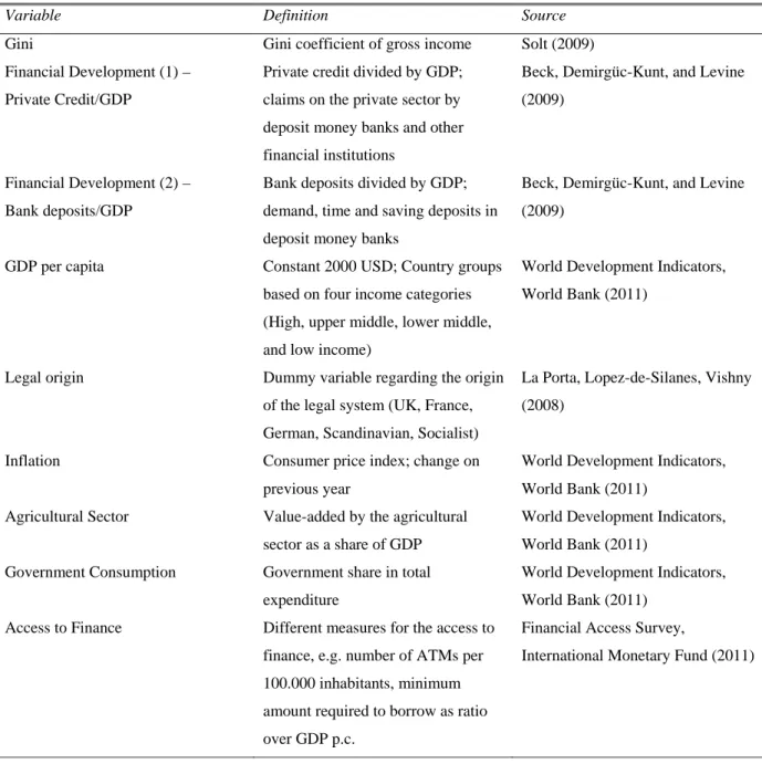
credit provided by deposit money banks and other financial institutions to the private sector. It does not include credit provided to the state or by central banks. Bank deposits is also based on the IMF’s International Financial Statistics and consists of demand, time and saving deposits in deposit money banks. Both variables are standard measures of financial development and used in the empirical literature described above. GDP per capita is used in constant USD and sourced from the World Development Indicators by the World Bank. Table 1 provides an overview of the definitions and sources of all variables used in our analysis.
Table 1: Overview of variables and sources
Variable Definition Source
Gini Gini coefficient of gross income Solt (2009) Financial Development (1) –
Private Credit/GDP
Private credit divided by GDP; claims on the private sector by deposit money banks and other financial institutions
Beck, Demirgüc-Kunt, and Levine (2009)
Financial Development (2) – Bank deposits/GDP
Bank deposits divided by GDP; demand, time and saving deposits in deposit money banks
Beck, Demirgüc-Kunt, and Levine (2009)
GDP per capita Constant 2000 USD; Country groups based on four income categories (High, upper middle, lower middle, and low income)
World Development Indicators, World Bank (2011)
Legal origin Dummy variable regarding the origin of the legal system (UK, France, German, Scandinavian, Socialist)
La Porta, Lopez-de-Silanes, Vishny (2008)
Inflation Consumer price index; change on previous year
World Development Indicators, World Bank (2011)
Agricultural Sector Value-added by the agricultural sector as a share of GDP
World Development Indicators, World Bank (2011)
Government Consumption Government share in total expenditure
World Development Indicators, World Bank (2011)
Access to Finance Different measures for the access to finance, e.g. number of ATMs per 100.000 inhabitants, minimum amount required to borrow as ratio over GDP p.c.
Financial Access Survey,
9
Private credit over GDP can be used as proxy for financial development as it reflects the ease to get credit for households and corporations. The more credit provided to the private sector, the easier it was for private institutions to signal their creditworthiness at the respective lending rate and the more private individuals were able to have access to credit markets. This argumentation does not always hold as can be seen with real estate credits and the subprime crisis in the United States in 2007-08. Furthermore we do not have micro level data regarding the distribution of credit in the population and among businesses and can consequently not asses how different groups in the population benefit from increasing credit provision and how those credits are used. Still we do believe that it is a good proxy for financial development as there is a high correlation between private credit over GDP and the access to finance measured by the number of ATMs or number of bank branches per population or per square mile.4 The alternative measure we use, bank deposits over GDP, serves as a proxy as it describes again the access to finance. Without or with less financial development, less people had access to bank accounts. Lower values of bank deposits over GDP also reflect the lack of trust of creditors in their financial system and their banks. There are again some caveats as we do not know the distribution of bank deposits among the population and businesses and we have no data on the turnover rate of the deposits. Overall, both measures explain how well the financial system performs its inherent task – channeling funds and intermediating between creditors and debtors.
Income inequality over time around the world
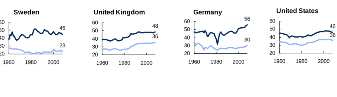
Income inequality measured as gini coefficient is normally distributed for the whole sample with a mean of 44.3, standard deviation of 9.6, skewness of .36 and kurtosis of 3.0. Income inequality in general changes only slowly over time. Splitting the sample in observations by year, the gini becomes more normally distributed over time with lower standard deviations. This process is accompanied by higher means. Figure A1 shows the distribution of inequality around the world measured as average over the years 2000 to 2004. Inequality is highest in Latin America and Southern Africa. Very high and increasing levels of inequality can also be observed in developed countries like Germany, the United Kingdom, and the United States. However the level of net income inequality, i.e. after redistribution is much lower in developed countries as shown in
4
10
figure 1. Even countries that are considered as being very equal, like Sweden, have a high level of gross income inequality. This examples shows that in discussing equality aspects one has to be explicit whether equality before or after redistribution is considered. As the returns to human capital investment and the founding of businesses are measured as gross income before taxes and redistribution, we regard only gross income inequality in our research. In Germany and Sweden net inequality is relatively constant compared to gross inequality in contrary to the United Kingdom and the United States, where net and gross inequality move parallel. The level of redistribution in those countries does not change when inequality increases or decreases.5
Figure 1: Inequality over time
The dark blue line shows the gross income inequality. The light blue line shows net income inequality.
Financial development over time around the world
Financial development defined by the measure of private credit over GDP is increasing over time. This process is more monotone than the development of gross inequality. The mean for the whole sample is .45 with a standard deviation of .39. Figure A2 shows the stage of financial development for the countries in our sample for the years 2000 to 2004. As expected, financial development is especially high in OECD countries with the highest levels in countries of Anglo-Saxon origin. The countries with the highest values are Iceland, Luxembourg, and the United States. The distribution of financial development across countries and time is not as normal as inequality so that we transform the variable with logs. This changes the skewness from 1.5 to -.3 and the kurtosis from 5.0 to 2.8.6 In contrast to inequality credit over GDP becomes more uniformly distributed across countries over time, when looking at different income country groups. So we do not observe a convergence to one level but rather that some countries keep lower levels while other countries increase their credit provision more quickly.
5
We will use the term inequality in the remainder of this paper to refer to gross income inequality 6
A normal distribution has a skewness of 0 and a kurtosis of 3
56 30 20 30 40 50 60 2000 1980 1960 Germany 48 36 20 30 40 50 60 2000 1980 1960 46 20 30 40 50 60 2000 1980 1960 36 45 23 60 50 40 30 20 2000 1980 1960
11
4 Econometric Estimation
Basic estimation
We test the hypothesis of Galor and Zeira (1993) and Banerjee and Newman (1993), namely that financial development has a negative impact on income inequality and the hypothesis of Greenwood and Jovanovic (1990) that the influence follows an inverted U-shape. Our basic estimation to compare this data with previous work is:
, , , . ., . ., ,
Following the hypothesis of a linear negative influence, should be negative and significant and should be insignificant. According to the inverted U-shape hypothesis, should be significant and positive and should be significant and negative. We add GDP per capita and its squared term to control for Kuznets curve. Therefore should be positive and significant and should be negative and significant. Gini is normally distributed and rather stable and consequently not transformed into logs. Both Credit and GDP p.c. are transformed into logs, as both variables have a skewed distribution. The square of the variables is taken from the log. Our control measure for financial development is Bank deposits which is also log-linearized and treated like Credit. We estimate the model with ordinary least squares (OLS). One impediment to our estimation is heteroskedasticity, which we handle by using heteroskedasticity robust standard errors. Furthermore there are different approaches on how to proceed with yearly data.7 Yearly data represent cyclical movements while using five-year averages yields a more balanced panel but at the same time means a loss of a lot of information. Table 2 shows a comparison of the two models for our basic estimation.
7
Romer and Romer (1999) and Jaumotte et al. (2008) use yearly data. Five year averages are taken by Clarke et al.
(2003), Li et al. (1998), and Kappel (2010). Beck et al. (2004) and Kappel (2010) do not use information provided by
yearly data or averages over several years and estimate the effect of financial development on income inequality
12
Table 2: Basic estimation
Income inequality measured as Gini coefficient is the dependent variable for all models. Model 1 is using yearly data and model 2 is using five-year averages. Model a is estimated with default heteroskedasticity robust standard errors. Model b uses cluster robust standard errors. Max/Min of Credit and GDP indicate at which level the sign of the explanatory variable changes. Neither country fixed effects nor time dummies are included in order to make the results comparable to previous research. The estimation with bank deposits as proxy for financial development is in table A5. Dep. var: Gini Model (1a) (1b) (2a) (2b) Credit -3.70339*** -3.70339 -3.17382 -3.17382 Credit² 0.69142*** 0.69142 0.58253*** 0.58253 GDP p.c. 12.9570*** 12.9570** 13.39131*** 13.39131*** GDP p.c.² -0.90697*** -0.90697*** -0.92665*** -0.92665*** Constant 6.37289 6.37289 3.90105 3.90105 N 3,228 3,228 802 802 R² 0.0719 0.0719 0.0656 0.0656 Max/Min of:
Credit (in %) 15% not significant strict. positive not significant
GDP (in USD) 1,265 1,265 1,374 1,374
***, **, * denote statistical significance levels at 1%, 5%, and 10%
Independent of the measure of financial development and the treatment of the use of yearly or five-year averaged data we confirm Kuznets hypothesis on the relation of economic development and income inequality. Inequality rises with increasing GDP per capita and falls after a certain level is reached. In the overall sample the maximum Gini is reached between 1,265 to 1,374 USD. This result is in line with Clarke et al. (2003) who estimate the maximum inequality between 1,250 and 2,350 USD. Using yearly data, financial development first lowers income inequality and after reaching a specific stage of development increases income inequality. For five-year averages financial development has a positive impact if it is approximated by credit. Using bank deposits as proxy for financial development, we do not see a significant effect on the income distribution in the basic estimation. These findings contradict the outcome of Clarke et al. and suggest that financial development works in the opposite way of what is suggested by the theory. In a second step we correct the default standard errors in the pooled OLS estimation for
13
clustered data.8 Cluster robust standard errors should to be used as the default standard errors assume that errors i are uncorrelated over i for fixed t. Kuznets curve remains apparent but the link of financial development and income inequality disappears. In order to perform a more thorough test of the theories named above, we make further adjustments on the basic estimation. We control for a time factors by using time dummy variables (cf. Table A1). This step increases the R² by about 6 percentage points in model 2 and by about 3 percentage points in model 1. The Kuznets curve still holds but the turning point for GDP per capita is a bit lower at about 1,140 USD. Financial development follows the same pattern as in the basic estimation, however all variables are highly significant when we do not control for clusters. This adjustment also leads to a significantly positive effect of financial development with cluster robust standard errors.
Econometric hurdles
Former research took endogeneity into account and used an instrumental variable approach to estimate the impact of financial development for the case that inequality influences financial development or in case of an omitted variable bias. Results did not differ from the OLS approach a lot. Instruments for financial development were in line with literature on financial development the origin of a country’s legal system. We follow the same approach and use legal origin
dummies as exogenous instruments. The first stage R² is 57% in our sample when we include
GDP p.c. and the time dummies. The fitted values for credit have a correlation of 76% with the original values and can consequently be viewed as having a good fit. However, the existing theories we test do not allow for an influence of inequality on financial development so that we do not pursue further attempts to correct for reverse causality in our robustness checks. An endogeneity problem might also occur due to omitted variables. We address this issue by using a fixed effects regression including time dummies. This is the main difference in our econometric approach from previous research. Country dummies are included to control for country specific characteristics that do not change over time but are potentially influential regarding income inequality. These can be cultural factors, religion, colonial background and others. Time dummies are included to control for common shocks for all countries like major political events
8
Clarke et al. (2003) and Kappel (2010) do not report what kind of standard errors they used. So we compare
14
or business cycle fluctuations in our explanatory variables, as we expect Credit and GDP p.c. to grow over time as countries become more developed and richer. Another problem often occurring in estimations is multicollinearity. Multicollinearity reduces the power of the OLS-estimator but the estimator is still unbiased and efficient. The Variance Inflation Factor (VIF) shows a high multicollinearity which is due to the structure of our base estimation with linear and squared terms of financial and economic development. Estimating the influence of financial and economic development on income inequality with either linear or squared terms reveals a low result for the VIF and confirms that multicollinearity is not an issue in the estimation.
The estimations in table 2 are object to an omitted variable bias since no country specific effects that explain income inequality are included. Thus, as a next step we control for country specific effects by conducting a fixed effect estimation. Fixed effects are not a cure for all omitted variable problems as time variant country characteristics are not included, but it is a good approach to tackle a potential omitted variable bias (cf. Acemoglu et al. (2008)). A further potential critique regarding the estimation process is endogeneity caused by reverse causality. One way to solve reverse causality is to use a two stage least squares (2SLS) estimation.
Within estimation
Key to our paper is the explanation of the influence of financial development on income inequality within and not between countries. To estimate this influence we use the fixed-effect estimator, also known as within estimator. The within estimator has the advantage of controlling for country characteristics and in contrast to the between estimator using all observations of the dataset and developments over time. The results of the within-estimation are shown in table 3. Although we do not believe that reverse causality is an issue regarding financial development we also report the results of a 2SLS estimation in table 3. As before, yearly data and five year averages produce similar coefficients. So we shall regard only yearly data in the remainder of this paper. Focusing on the sole effect of GDP per capita and financial development we do neither observe a Kuznets curve nor non-linear effects of financial development.
15
Table 3: Fixed effect and 2SLS estimation
Model 3 is using yearly data and model 4 is using five-year averages. Model a is estimated with fixed effects. Model b is also a fixed effects model but uses 2SLS with legal origin dummies as instruments in the first stage regression. Both models are calculated with heteroskedasticity robust standard errors. Max/Min of Credit and GDP p.c. indicate at which level the sign of the explanatory variable changes. Both models include time dummies. The estimation with bank deposits as proxy for financial development is in table A5.
Dep. var: Gini
Model
(3a) fixed effect (3b) fe-2SLS (4a) fixed effect (4b) fe-2SLS
Credit 2.2863*** -28.5547*** 2.5671*** omitted (collinear.)
Credit² not significant1 3.3789*** not significant1 omitted (collinear.) GDP p.c. -21.1659*** 20.0077* -24.0970*** -14.2786*** GDP p.c.² 1.3970*** -0.8969 1.5619*** 1.1003*** Constant 122.3372*** 0.7713 133.9544*** 94.5933*** N 3228 3896 802 968 R² 0.1793 0.1692 0.247 0.1972 Max/Min of:
Credit (in %) strict. positive 68.4% strict. positive ---
GDP (in USD) 1.950 strict. positive 2,240 658
***, **, * denote statistical significance levels at 1%, 5%, and 10%
1both terms for credit are insignificant in a quadratic estimation so that the credit only enters linearly in the model
Independent of the time specification and the inclusion of dummy variables we reject the hypothesis that financial development is monotonously reducing inequality. Enhanced credit provision benefits the poor more than the rich only for very low levels of private credit to GDP. Estimating a more thorough model leads to the same result, the rejection of a negative influence of financial development on income inequality. The idea of the first part of Greenwood and Jovanovic (1990) that the use of financial intermediation does not hamper poor but favor rich people is supported in parts by this analysis and also holds when using bank deposits as proxy. While the fixed effects model estimates a strictly positive impact the instrumental variable approach can explain both models for a certain range of financial development. Until a credit provision to GDP of 68%, financial development reduces inequality which backs Galor and Zeira and Banerjee and Newman. Inequality increases after this threshold which might be due to different investment opportunities as argued by Greenwood and Jovanovic. Our model that
16
corrects for fixed effects has a within R² of 18%. So besides the high significance level of all included variables we can explain a large part of within country variation in inequality by financial development. A surprising result of the analysis is the inverted U-shape of GDP per capita. When the average income rises, inequality falls only until a level of about 1,950 to 2,240 USD and rises afterwards.
Robustness checks
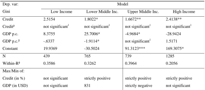
We conduct several robustness checks in order to control for the validity of our results. These checks include estimations for subsamples of countries, the inclusion of different control variables and further support for the ratio of private credit over GDP as measure for financial development. Due to the large database we are able to investigate whether the effects on income inequality hold for different country groups. Therefore we split the sample into four groups according to the income categories defined by the World bank. The high income group consists of 1285 country-year observations, the upper middle income group of 739, the lower middle income group of 765, and the low income group of 439. All estimations are performed with within-estimators and yearly data, including time dummies to identify the influence of financial and economic development on the variation of income inequality independent of a time factor and country specific characteristics. Robust standard errors are used when necessary. We expect the signs of the coefficients for economic and financial development as follows:
Table 4
Low Inc. Lower Middle Inc. Upper Middle Inc. High Income Rational GDP Positive positive
Or positive negative or Positive negative Kuznets GDP² Insig. insig. negative insig. Negative insig.
FD Positive positive
Or positive positive or Positive positive or negative Greenw. & Jovan. FD² Insig. insig. negative insig. Negative negative insig.
Depending on the exact turning point in the models of Kuznets and Greenwood and Jovanovic the squared term of financial development in the lower and upper middle income group might be insignificant. Table 5 shows the estimation results by country group.
17
Table 5: Fixed effect estimation by income group
All estimations are fixed effect estimations with time dummies and robust standard errors. Max/Min of Credit and GDP indicate at which level the sign of the explanatory variable changes.
Dep. var: Gini
Model
Low Income Lower Middle Inc. Upper Middle Inc. High Income
Credit 2.5154 1.8022* 1.6672** 2.4138**
Credit² not significant1 not significant1 not significant1 not significant1
GDP p.c. 8.3755 25.7006* -4.9684* -28.9424 GDP p.c.² -.6337 -1.9114* not significant1 1.5171 Constant 19.9369 -30.5024 91.3123*** 169.3075* N 439 765 739 1285 Within-R² 0.3586 0.3262 0.3964 0.2056 Max/Min of:
Credit (in %) not significant strictly positive strictly positive strictly positive GDP (in USD) not significant 831 strictly negative not significant ***, **, * denote statistical significance levels at 1%, 5%, and 10%
1both terms for credit are insignificant in a quadratic estimation so that the credit only enters linearly in the model
By combining the income groups we can observe Kuznets curve, although GDP is not a significant explanatory variable in low and high income countries:
Figure 1: Economic development and income inequality
Gini GDP p.c. Upper Middle Income High Income Low Income Lower Middle Income Original Kuznet’s curve insignificant insig- nifi- cant
18
The relation of financial development and income inequality is close to Greenwood and Jovanovic. In all but low income countries rich people profit more from a higher distribution of credit than poor people. For low income countries financial development is not a relevant factor for income inequality. Although the ratio of credit over GDP is significant, the absolute effect is low. With credit being measured in logs and Gini in absolute levels a coefficient of 2.4 means that a 10% increase in credit leads to a 0.24 increase of the Gini. Estimating the different income groups with interaction terms instead of subsamples confirms that financial development has a significant high positive effect for high income countries and a significant positive but lower effect for upper middle income countries. Lower middle income and low income countries’ interaction terms are not significant.
For further robustness checks besides the analysis of subsamples we use different control variables. One control variable we include is legal origin as dummy when not using the fixed effect estimation. Legal origin is a standard instrument in the financial development literature. La Porta, Lopez-de-Silanes, and Shleifer (2007) give a detailed overview of research dealing with the importance of legal origins for economic development and explain the differences of legal systems. They also address the criticism related to legal origin as an instrument but conclude in their “Legal Origins Theory” that this variable is significant in explaining growth. Legal origin is of importance for explaining differences in income inequality as it also reflects cultural and historical factors. La Porta et al. (2007, p.37) see the French civil law family as more concerned with market failure and “as a system of social control of economic life”. In contrast the common law family, originated in Britain, deals more with state abuse.9 As the civil law family more mirrors social concerns it is more likely to be associated with lower income inequality. So we add
legal origin in our base regression as a control variable. Including legal origin dummy variables gives a higher R², which increases from 7% to 14% in the basic estimation and to 17% if year dummies are included.10 French and German legal origins – the civil law family – reduce inequality significantly by 3.5 and 7.9 points. UK origin does not have a significant effect. Using bank deposits instead of credit over GDP as proxy reveals similar results. Credit reduces inequality in this estimation only until a very low level and increases inequality afterwards. This result is supported by the correlation coefficients of income inequality and private credit over
9
There are two major legal systems in the world. Common law (British origin) and civil law, that can further be
distinguished in French, German, and Scandinavian civil law. 10
19
GDP. In the category of high income countries, Anglo-Saxon countries are disproportionally represented among the top positive correlations: United Kingdom (N=49, 0.92), New Zealand (N=45, 0.91), Canada (N=46, 0.84), United States (N=49, 0.78), and Australia (N=49, 0.66) all have a large number of observations and very high correlations of income inequality and the provision of private credit. Further control variables we add in our within estimation are inflation, the share of government consumption and the share of the agricultural sector in total GDP. Inflation should have a positive sign if the upper class with access to financial instruments could protect its wealth against inflation and the working class was more severely hit due to sticky wages. Government consumption was included in previous research as a higher government share reflects the magnitude of redistribution. We do not expect a significant sign as this is relevant for the net income inequality but does influence gross income inequality. The share of the agricultural sector in total GDP, which could also be replaced by the share of the modern sector, is important as more agricultural work is often associated with more inequality due to the low skill workers employed in the agricultural sector. Depending on the combination of these control variables, whether all or just some are included, variables change the size of the coefficients and partly the significance level, but the key result persists: Depending on the exact model specification financial development either does not influence income inequality at all or has a positive effect and increases the gini coefficient.11 Another check we do is to control for a steady time trend instead of using year dummies. The time trend assumes a constant development from the 1960s to the 2000s but is not appropriate to measure effects of single years. The time trend turns out be significant and negative, implying that inequality is generally reduced over the last 50 years. This is also supported by the year dummies, of which most are significant and negative and of which the size increases especially in the 1980s. Still, the inequality increasing effect of financial development persists. Using lagged variables of the explanatory variables to address a time lag in the relation with inequality does not improve our fit. The significance levels are similar as well as the sign of the coefficients but the size of the coefficients is reduced and the R² decreases.
The main critic to our research concerns the measure of financial development. Does the magnitude of credit provision really indicate financial development? We strongly believe yes. First, the amount of credit over GDP indicates the level of financial intermediation. If financial
11
20
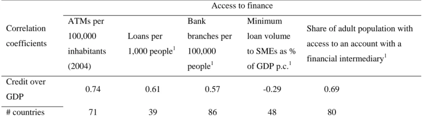
intermediaries were not able to assess credit risk, to overcome a maturity mismatch and to pool savings, they would provide less credit to households and enterprises. Second, the amount of credit could be biased towards few borrowers with high amounts outstanding and many borrowers with low amounts of credit and even more potential borrowers with no access to finance at all. We address this argument which aims at the question whether the amount of credit mirrors the access to finance by investigating the link of access to finance and the ratio of credit over GDP. The IMF’s Financial Access Survey (2011) and Demirgüc-Kunt and Beck (2007) provide different measures for the access to financial intermediaries. Correlations of these measures with credit are shown in table 6.
Table 6: Access to finance and the provision of credit
The number of ATMs is taken from the IMF’s Financial Access Survey. The other measures are taken from the World bank. Correlation coefficients Access to finance ATMs per 100,000 inhabitants (2004) Loans per 1,000 people1 Bank branches per 100,000 people1 Minimum loan volume to SMEs as % of GDP p.c.1
Share of adult population with access to an account with a financial intermediary1
Credit over
GDP 0.74 0.61 0.57 -0.29 0.69
# countries 71 39 86 48 80
1Year may differ by country, credit over GDP is taken as average from 1999 to 2003
The measures for access to finance are only available as cross section and not as panel data and differ with regards to the number of countries covered. The number of ATMs per 100,000 inhabitants indicates how many people use bank accounts. If credit and bank access were only relevant for few, there were less ATMs. The correlation of 0.74 for a set of 71 countries backs our use of credit as proxy for financial development. The number of bank branches and number of loans point in the same direction. If only a small proportion of the population would use financial intermediaries for the provision of credit, there were fewer banks and fewer loans. Financial development in the sense of Banerjee and Newman (1993) means that funding for small and medium enterprises gets easier. Especially small loans would help start a business or grow a small business. The minimum loan volume should also be lower in better developed financial
21
markets as more credit processes should be more efficient and worthwhile for banks even for relatively lower amounts of credit. The negative correlation of minimum loan volume with total credits confirms this. The lower the minimum credit volumes are the higher is the provision of credit. The fifth indicator we use is based on survey data and measures the overall access of the adult population to a bank account. Even developed countries in the European Union have values below 100% as some people abstain from banking voluntarily or involuntarily due to discrimination or the fee structure. Again, more people using financial services are correlated with higher amounts of credit. All these correlations over different measures and different sets of countries support the use of the private credit over GDP ratio as proxy for financial development.
5 Conclusion
Two phenomena can be observed over the last five decades around the world – increasing financial development and increasing gross income inequality in many countries, especially in the developed world. We presented theoretical models which explain the link of financial development and income inequality and predict that more developed financial markets lead to decreasing levels of income inequality regarding labor and entrepreneurial income and first increasing and then decreasing levels regarding capital income. Earlier empirical research focusing on this financial development versus income inequality nexus confirmed the decreasing effect of financial development. This research is either built upon a pure cross-country perspective that cannot account for the many country inherent characteristics, or used panel data approaches but again neglecting country characteristics.
Using a broader data set and time-invariant country specifics in our panel estimation, we reach a different conclusion in the analysis of this nexus and reject those earlier theories and previous empirical research. Integrating time-invariant country characteristics we find a positive relation between financial development and income inequality within countries. More developed financial markets lead to higher gross income inequality. This holds for several robustness checks, e.g. for subsamples by different income groups, neglecting country characteristics and including further control variables, as well as bank deposits as an alternative measure for financial development. The positive relation is highly significant but only of small magnitude. An increase of the provision of credit by ten percent leads to an increase in the gini coefficient by 0.23 for the within
22
estimation.12 We do not exclude the possibility that all income groups within a country benefit from more financial development, but we do find that those who are already better off benefit more because income inequality is increasing. These results add to the existing literature on financial development and income inequality by using new estimation techniques and a dataset with more countries for a longer time horizon compared to previous research. Still, the relationship between finance, financial development and income inequality offers more research opportunities. Work on the development of top incomes (e.g. Kaplan and Rauh (2010), Atkinson et al. (2009)) shows how the top earners increased their share of overall income in developed and developing countries and disaggregates for example income types or professions of these top earners. As capital income is not the main source for increasing income of the super rich, the channels from more financial development to higher income inequality are subject to future research.
12
23
References
Acemoglu, Daron; Johnson, Simon; Robinson, James A.; Yared, Pierre (2008): Income and Democracy. In: American Economic Review 98 (3), S. 808–42.
http://ideas.repec.org/a/aea/aecrev/v98y2008i3p808-42.html
Atkinson, Anthony B.; Piketty, Thomas; Saez, Emmanuel (2009): Top Incomes in the Long Run of History. (NBER Working Paper Series, 15408). http://www.nber.org/papers/w15408
Banerjee, Abhijit V.; Newman, Andrew F. (1993): Occupational Choice and the Process of Development. In: Journal of Political Economy 101 (2), S. 274–98.
http://ideas.repec.org/a/ucp/jpolec/v101y1993i2p274-98.html
Beck, Thorsten; Demirgüc-Kunt, Asli; Levine, Ross (2004): Finance, Inequality, and Poverty: Cross-Country Evidence (NBER Working Papers, 10979).
http://ideas.repec.org/p/nbr/nberwo/10979.html
Demirgüç-Kunt, A.; Beck, T. H. L. (2008): Finance for all?: Policies and pitfalls in expanding access (Open Access publications from Tilburg University).
http://ideas.repec.org/p/ner/tilbur/urnnbnnlui12-3508393.html
Beck, Thorsten; Demirgüç-Kunt, Asli; Levine, Ross (2010): Financial Institutions and Markets across Countries and over Time: The Updated Financial Development and Structure
Database. In: World Bank Economic Review 24 (1), S. 77–92.
http://ideas.repec.org/a/oup/wbecrv/v24y2010i1p77-92.html
Clarke, George; Xu, Lixin Colin; Zou, Heng-fu (2003): Finance and income inequality. Test of alternative theories (Policy Research Working Paper Series, 2984).
24
Deininger, Klaus; Squire, Lyn (1996): A New Data Set Measuring Income Inequality. In: World Bank Economic Review 10 (3), S. 565–91.
http://ideas.repec.org/a/oup/wbecrv/v10y1996i3p565-91.html
Demirgüc-Kunt, Asli; Levine, Ross (2009): Finance and Inequality: Theory and Evidence. In:
Annual Review of Financial Economics 1 (1), S. 287–318.
http://ideas.repec.org/a/anr/refeco/v1y2009p287-318.html
Galor, Oded; Zeira, Joseph (1993): Income Distribution and Macroeconomics. In: Review of Economic Studies 60 (1), S. 35–52. http://ideas.repec.org/a/bla/restud/v60y1993i1p35-52.html
Greenwood, Jeremy; Jovanovic, Boyan (1990): Financial Development, Growth, and the Distribution of Income. In: Journal of Political Economy 98 (5), S. 1076–1107.
http://ideas.repec.org/a/ucp/jpolec/v98y1990i5p1076-1107.html
International Monetary Fund (IMF) (2011): Financial Access Survey. http://fas.imf.org
Kaplan, S. N.; Rauh, J. (2010): Wall Street and Main Street: What Contributes to the Rise in the Highest Incomes? In: Review of Financial Studies 23 (3), S. 1004–1050.
Kappel, Vivien: The Effects of Financial Development on Income Inequality and Poverty (10/127). http://econpapers.repec.org/RePEc:eth:wpswif:10-127
Kuznets, Simon (1955): Economic Growth and Income Inequality. In: The American Economic Review 45 (1), S. 1–28. http://www.jstor.org/stable/1811581
La Porta, Rafael; Lopez-de-Silanes, Florencio; Shleifer, Andrei (2008): The Economic Consequences of Legal Origins. In: Journal of Economic Literature 46 (2), S. 285–332.
25
Levine, Ross (2005): Finance and Growth: Theory and Evidence. In:, Bd. 1: Elsevier (Handbook of Economic Growth), S. 865–934. http://ideas.repec.org/h/eee/grochp/1-12.html
Li, Hongyi; Squire, Lyn; Zou, Heng-fu (1998): Explaining International and Intertemporal Variations in Income Inequality. In: Economic Journal 108 (446), S. 26–43.
http://ideas.repec.org/a/ecj/econjl/v108y1998i446p26-43.html
Ortiz, Isabel; Cummins, Matthew: Global Inequality: Beyond the Bottom Billion - A Rapid Review of Income Distribution in 141 Countries (1102).
http://ideas.repec.org/p/uce/wpaper/1102.html
Papageorgiou, Chris; Lall, Subir; Jaumotte, Florence: Rising Income Inequality: Technology, or Trade and Financial Globalization? (08/185).
http://ideas.repec.org/p/imf/imfwpa/08-185.html
Romer, Christina D.; Romer, David H. (1999): Monetary policy and the well-being of the poor. In: Economic Review (Q I), S. 21–49. http://ideas.repec.org/a/fip/fedker/y1999iqip21-49nv.84no.1.html
Solt, Frederick (2009): Standardizing the World Income Inequality Database. In: Social Science Quarterly 90 (2), S. 231–242.
World Bank, 2010, World Development Indicators. World Bank, Washington D.C.
26
Appendix Tables
Table A1: Correlation analysis
Complete Dataset (N=3228)
Gini Credit GDP p.c.
Gini 1.000 Credit -0.089*** 1.000
GDP p.c. -0.145*** 0.753*** 1.000
High Income (N=1285) Upper Middle Income (N=739)
Gini Credit GDP p.c. Gini Credit GDP p.c.
Gini 1.000 1.000 Credit 0.142*** 1.000 0.298*** 1.000 GDP p.c. 0.048*** 0.642*** 1.000 0.054 0.235*** 1.000 Gini 1.000 1.000 Credit -0.083** 1.000 0.048 1.000 GDP p.c. 0.242*** 0.511*** 1.000 0.256*** 0.259*** 1.000
Lower Middle Income (N=765) Low Income (N=439)
*,**,*** represent the significance level of the correlation coefficient (10%, 5%, and 1%); the correlations were computed in Stata by correlate, the significance level was calculated by pwcorr, sig
27
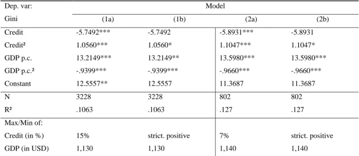
Table A2: Basic estimation including year dummies
Income inequality measured as Gini coefficient is the dependent variable for all models. Model 1 is using yearly data, model 2 is using five-year averages. Model a is estimated with default heteroskedasticity robust standard errors. Model b uses cluster robust standard errors. Max/Min of Credit and GDP indicate at which level the sign of the explanatory variable changes. No country fixed effects are included in order to make the results comparable previous research, however year dummies are included.
Dep. var: Gini Model (1a) (1b) (2a) (2b) Credit -5.7492*** -5.7492 -5.8931*** -5.8931 Credit² 1.0560*** 1.0560* 1.1047*** 1.1047* GDP p.c. 13.2149*** 13.2149** 13.5980*** 13.5980*** GDP p.c.² -.9399*** -.9399*** -.9660*** -.9660*** Constant 12.5557** 12.5557 11.3687 11.3687 N 3228 3228 802 802 R² .1063 .1063 .127 .127 Max/Min of:
Credit (in %) 15% strict. positive 7% strict. positive
GDP (in USD) 1,130 1,130 1,140 1,140
***, **, * denote statistical significance levels at 1%, 5%, and 10%
Table A3: First stage regression - credit
Legal origin dummies for common law, French civil law, German civil law, and Scandinavian civil law are used as instruments in the first stage regression to predict private credit. Time dummies are included in the regression but not reported. GDP p.c. is in logs.
Dep. var: Credit Coefficient Rob. Standard Error z-Value p-Value
Legal origin UK 0.5686 0.2407 2.36 0.018
Legal origin FR 0.3737 0.2437 1.53 0.125
Legal origin GE 0.1809 0.1939 0.93 0.351
Legal origin SC omitted because of collinearity
GDP p.c. 0.6389 0.0622 10.27 0.000 Constant -2.7643 0.6569 -4.21 0.000 N 3222 R² - within 0.4028 R² - between 0.6397 R² - overall 0.5732
28
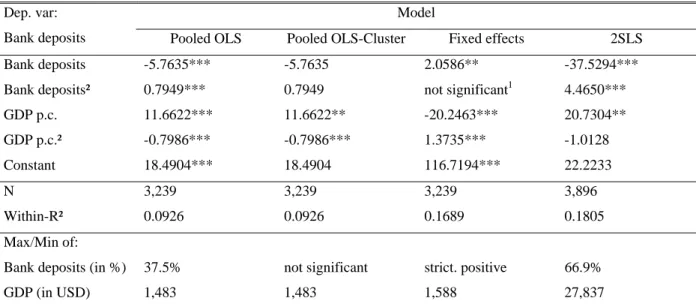
Table A4: Robustness check with Bank deposits
Bank deposits are used as proxy for financial development. All models are estimated with time dummies and robust standard errors.
Dep. var: Bank deposits
Model
Pooled OLS Pooled OLS-Cluster Fixed effects 2SLS Bank deposits -5.7635*** -5.7635 2.0586** -37.5294*** Bank deposits² 0.7949*** 0.7949 not significant1 4.4650*** GDP p.c. 11.6622*** 11.6622** -20.2463*** 20.7304** GDP p.c.² -0.7986*** -0.7986*** 1.3735*** -1.0128 Constant 18.4904*** 18.4904 116.7194*** 22.2233 N 3,239 3,239 3,239 3,896 Within-R² 0.0926 0.0926 0.1689 0.1805 Max/Min of:
Bank deposits (in %) 37.5% not significant strict. positive 66.9%
GDP (in USD) 1,483 1,483 1,588 27,837
***, **, * denote statistical significance levels at 1%, 5%, and 10%
1 Both terms of bank deposit in the quadratic form are insignificant, but bank deposits is significant in its linear form
Table A5: First stage regression – bank deposits
Legal origin dummies for common law, French civil law, German civil law, and Scandinavian civil law are used as instruments in the first stage regression to predict bank deposits. Time dummies are included in the regression but not reported. GDP p.c. is in logs.
Dep. var: Bank
deposits Coefficient Rob. Standard Error z-Value p-Value
Legal origin UK 0.6834 0.2035 3.36 0.001
Legal origin FR 0.4298 0.1944 2.21 0.027
Legal origin GE 0.3549 0.1616 2.20 0.028
Legal origin SC omitted because of collinearity
GDP p.c. 0.5327 0.0524 10.16 0.000 Constant -1.7323 0.5788 -2.99 0.003 N 3233 R² - within 0.4482 R² - between 0.6399 R² - overall 0.5656
29
Table A7: Income inequality and financial development by country
Only country-year observations with information on income inequality (Gini), financial development (credit), and GDP per capita are included in the table, as other information were not used for the estimation.
Gini Credit
Country N Mean Min Max Mean Min Max
High Income 1285 42.84 25.01 64.37 74.57 7.04 269.76 Australia 44 39.76 31.29 43.96 50.24 19.31 121.43 Austria 33 42.85 33.08 51.81 80.59 38.14 111.58 Bahamas, The 32 54.05 48.20 61.43 50.96 31.85 69.94 Barbados 28 45.56 40.46 52.16 40.93 31.01 49.94 Belgium 36 34.01 25.01 51.29 45.82 11.23 93.70 Canada 46 39.46 35.82 43.82 78.13 17.73 183.83 Croatia 14 34.87 32.40 38.21 42.67 24.98 67.32 Cyprus 19 42.59 37.00 47.44 140.18 91.21 200.80 Czech Republic 15 35.50 33.58 36.81 48.72 29.21 69.25 Denmark 47 48.70 45.43 54.55 54.76 22.02 209.82 Estonia 16 48.79 43.93 51.56 41.50 9.47 99.25 Finland 44 42.96 36.38 64.37 55.73 37.18 93.26 France 35 42.22 31.28 54.70 73.82 22.36 106.75 Germany 37 46.36 31.43 55.95 91.10 63.09 116.93 Greece 41 44.67 38.55 55.23 37.04 13.48 91.66 Hong Kong 16 54.37 47.17 59.54 146.53 124.36 176.76 Hungary 26 41.00 28.16 48.28 33.78 16.18 64.21 Iceland 4 41.65 40.31 43.01 181.12 116.44 269.76 Ireland 44 44.45 38.87 47.43 70.71 30.42 205.77 Israel 30 41.29 30.67 45.08 57.34 31.66 88.39 Italy 42 45.23 38.18 51.12 64.67 47.56 103.33 Japan 45 37.87 34.26 41.70 126.38 51.27 200.61 Korea, Rep. 38 39.69 35.16 45.97 84.09 36.41 144.59 Latvia 15 47.19 42.15 53.20 34.42 7.04 94.72 Luxembourg 31 36.39 27.55 43.96 102.30 56.07 211.42 Malta 8 45.75 43.65 48.62 106.02 101.81 112.37 Netherlands 43 41.48 37.54 53.74 101.34 41.61 192.60 New Zealand 45 40.03 33.07 47.00 60.55 23.76 140.14 Norway 42 42.32 37.74 48.13 85.28 58.16 113.89 Poland 19 41.13 34.01 47.97 23.70 14.87 40.55 Portugal 32 53.44 46.42 61.05 90.08 47.99 171.69 Singapore 44 46.98 42.30 53.13 87.45 35.03 135.74 Slovak Republic 15 33.98 29.75 36.83 40.90 29.60 52.87 Slovenia 17 33.55 29.20 35.35 38.03 19.45 80.95 Spain 35 38.81 32.93 46.65 87.25 63.67 188.49 Sweden 49 44.60 36.94 51.09 89.64 51.37 134.88 Switzerland 26 42.29 39.17 56.64 146.44 100.84 162.99 Trinidad a. Tobago 34 44.69 37.83 64.06 39.84 12.28 62.16 United Kingdom 49 43.30 37.30 48.78 70.33 16.05 189.56 United States 49 43.50 39.33 47.93 116.43 70.53 210.73
30
Gini Credit
Country N Mean Min Max Mean Min Max
Upper Middle Income 739 49.49 27.52 77.28 32.31 2.80 155.25
Albania 10 32.27 30.62 35.13 5.46 2.80 11.81 Algeria 23 37.71 35.28 40.75 26.11 4.14 68.29 Argentina 22 46.20 43.04 50.38 16.17 9.77 25.18 Botswana 24 55.86 52.60 59.64 12.68 6.54 19.65 Brazil 17 56.45 52.66 58.53 35.26 27.03 54.49 Bulgaria 17 32.62 27.52 38.39 34.22 8.94 68.19 Chile 30 52.76 50.91 54.45 52.84 11.08 74.34 Colombia 41 58.53 48.86 67.50 25.34 16.83 35.65 Costa Rica 38 48.55 43.30 60.89 22.45 10.47 51.96 Dominica 1 41.41 41.41 41.41 63.30 63.30 63.30 Dominican Republic 22 48.86 45.91 50.44 22.20 14.80 30.75 Fiji 17 52.46 50.30 54.29 26.51 18.04 38.25 Gabon 8 57.68 42.74 70.66 12.82 7.89 16.37 Grenada 1 53.19 53.19 53.19 67.08 67.08 67.08 Iran 35 47.26 42.95 53.25 28.16 18.64 43.62 Jamaica 37 59.57 47.56 77.28 22.95 13.15 30.66 Kazakhstan 13 37.11 34.01 41.94 14.72 4.97 36.83 Lithuania 15 47.83 47.07 48.71 23.30 10.22 61.23 Macedonia, FYR 14 32.88 29.72 38.94 23.66 17.38 37.01 Malaysia 38 51.85 40.32 67.17 75.53 7.10 155.25 Mauritius 31 47.98 39.73 56.62 38.34 20.63 72.35 Mexico 42 51.49 46.72 68.75 20.36 8.69 37.10 Panama 44 52.22 47.97 57.37 51.24 10.51 97.32 Peru 20 47.65 44.34 51.01 16.94 3.16 27.89 Romania 12 43.19 40.46 49.79 14.45 6.43 36.87 Russian Federation 16 47.48 43.48 51.34 18.78 6.78 48.54 Serbia 6 41.13 40.29 41.77 22.01 16.31 27.98 Seychelles 1 57.59 57.59 57.59 22.45 22.45 22.45 South Africa 38 65.45 61.70 70.24 80.68 43.44 132.56 St. Lucia 2 49.75 40.25 59.26 67.72 58.26 77.19
St. Vincent and the Gren. 1 66.41 66.41 66.41 43.94 43.94 43.94
Suriname 7 50.28 50.05 50.51 14.33 7.27 21.88
Turkey 25 45.36 41.75 50.84 14.67 10.91 18.79
Uruguay 28 41.39 40.10 43.00 33.56 19.99 67.05
31
Gini Credit
Country N Mean Min Max Mean Min Max
Lower Middle Income 765 46.64 30.43 77.36 27.48 1.14 165.96 Angola 6 60.34 60.06 60.61 3.12 1.14 4.45 Armenia 15 45.68 39.59 54.42 7.86 3.09 23.42 Belize 7 55.57 50.58 59.07 41.33 37.26 46.80 Bhutan 3 48.17 48.07 48.27 14.60 11.48 18.08 Bolivia 22 53.61 44.10 58.26 38.22 4.47 63.04 Cameroon 19 47.69 43.96 49.51 16.93 6.66 28.14 Cape Verde 17 50.06 42.35 55.89 24.15 3.02 41.13 Cote d'Ivoire 32 48.89 38.20 59.84 28.93 14.91 41.22 Ecuador 28 50.59 42.81 61.64 21.63 12.91 40.67
Egypt, Arab Rep. 41 36.32 32.71 51.35 25.89 11.43 53.38
El Salvador 42 51.16 47.46 63.71 28.01 16.82 43.53 Georgia 10 45.44 43.14 47.55 6.45 3.31 11.31 Guatemala 29 54.27 42.14 57.89 17.43 11.25 29.04 Guyana 5 44.62 43.94 45.60 41.49 23.17 54.89 Honduras 24 55.94 52.46 72.79 31.34 13.84 46.60 India 46 35.35 31.99 44.51 19.46 7.84 36.37 Indonesia 29 34.98 32.19 38.59 28.29 9.04 53.53 Jordan 30 39.88 35.08 48.67 63.62 32.15 83.50 Lesotho 18 59.67 51.95 64.54 13.78 5.60 20.05 Moldova 13 41.22 37.24 44.46 14.78 4.45 29.68 Mongolia 11 35.69 34.15 38.72 13.49 6.25 32.63 Morocco 38 47.48 37.71 69.06 31.34 11.74 60.91 Nigeria 35 50.80 43.40 65.16 11.20 3.33 18.93 Pakistan 43 39.05 30.43 44.15 21.92 12.83 27.57
Papua New Guinea 11 49.05 40.62 52.56 15.07 12.37 17.95
Paraguay 19 50.98 37.51 55.35 22.09 13.18 29.03 Philippines 45 55.42 45.83 61.30 30.64 16.94 54.06 Senegal 17 44.93 39.50 58.56 18.13 14.51 26.10 Sri Lanka 27 45.33 32.52 57.22 18.55 7.74 28.71 Swaziland 13 55.25 49.07 77.36 14.14 10.92 18.83 Thailand 36 50.18 43.98 60.27 68.38 15.07 165.96 Tunisia 18 41.01 39.03 42.02 60.64 48.67 66.60 Vietnam 11 37.60 36.34 38.64 36.33 17.23 64.37 Yemen, Rep. 5 36.51 32.24 39.03 5.64 4.67 6.47
32
Gini Credit
Country N Mean Min Max Mean Min Max
Low Income 439 46.91 29.70 75.08 12.23 1.10 41.41 Bangladesh 10 34.08 33.16 35.75 24.41 15.12 31.14 Benin 4 37.43 36.89 37.97 13.59 12.05 15.11 Burkina Faso 10 50.79 44.77 54.31 9.40 5.73 12.84 Burundi 15 37.40 34.17 41.02 19.81 14.25 27.95 Cambodia 10 44.64 43.77 45.73 5.52 3.14 7.64
Central African Rep. 2 61.41 60.96 61.86 5.14 4.50 5.78
Chad 4 40.85 40.75 40.92 3.35 2.77 3.96
Congo, Dem. Rep. 2 44.70 44.52 44.88 1.88 1.58 2.19
Ethiopia 25 37.64 30.39 44.22 18.45 9.90 30.20 Gambia, The 12 52.54 48.15 59.91 13.55 8.88 26.07 Ghana 25 38.69 35.59 42.79 6.98 1.40 15.52 Guinea-Bissau 15 43.72 36.30 54.61 4.08 1.49 7.62 Haiti 11 54.06 53.61 56.05 12.74 10.26 13.99 Kenya 39 61.34 49.80 75.08 25.82 12.19 34.96 Kyrgyz Republic 12 42.60 39.00 47.30 5.97 3.74 11.29 Lao PDR 11 34.88 31.10 37.16 7.14 3.63 9.19 Madagascar 30 45.24 40.00 46.88 13.86 7.88 21.24 Malawi 25 58.57 39.45 72.33 11.14 4.95 20.12 Mali 18 44.17 37.51 53.00 13.48 8.13 17.11 Mauritania 14 43.66 38.79 47.50 25.61 16.53 41.41 Mozambique 10 42.82 40.15 46.01 11.27 8.31 15.39 Nepal 29 42.59 29.70 63.98 14.55 3.72 28.31 Niger 14 45.95 40.58 50.51 6.06 3.54 11.79 Rwanda 6 46.96 45.85 48.08 10.60 10.16 11.04 Sierra Leone 32 58.14 45.31 67.51 3.98 1.89 7.78 Tanzania 12 39.55 36.06 44.50 7.97 3.08 15.09 Togo 2 35.13 35.13 35.14 16.52 16.48 16.57 Uganda 20 41.82 37.01 46.09 3.94 1.10 5.87 Zambia 20 53.90 46.48 57.71 6.35 3.69 8.69
33
Figures
Figure A1: Income Inequality around the world
Income inequality measured by the gini coefficient of gross income. Data is based on averages from 2000 to 2004.
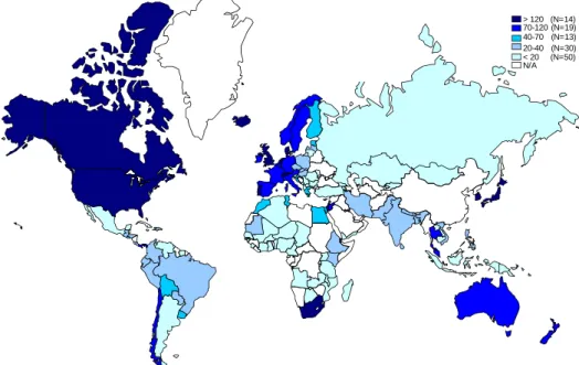
Figure A2: Financial Development around the world
Financial development measured by the average volume of private credit over GDP from 2000 to 2004
Figure A3: Financial Development, Economic Development, and Income Inequality > 50 (N=31) 45-50 (N=36) 40-45 (N=41) 35-40 (N=26) < 35 (N=14) Gross Gini Ø 2000-04 N/A > 120 (N=14) 70-120 (N=19) 40-70 (N=13) 20-40 (N=30) < 20 (N=50) N/A
34
3D-graphs for the relation of Gini, economic and financial development – All countries
Log of Credit over GDP Log of const. GDP (USD)
Gi n i ( g ro ss )