ABSTRACT
MULEY, NAMAN GAUTAM. A Closed Loop Approach to Virtual Machine Placement Algorithms. (Under the direction of Yannis Viniotis.)
© Copyright 2014 by Naman Gautam Muley
A Closed Loop Approach to Virtual Machine Placement Algorithms
by
Naman Gautam Muley
A thesis submitted to the Graduate Faculty of North Carolina State University
in partial fulfillment of the requirements for the Degree of
Master of Science
Computer Networking
Raleigh, North Carolina 2014
APPROVED BY:
Mihail Sichitiu Michael Devetsikiotis
Yannis Viniotis
DEDICATION
BIOGRAPHY
I have found that learning concepts and ideas is a worthy endeavour. Throughout my life, the people who have made me see miraculous insights, have been the people who have had profound impact on my thoughts. Being born in the hard working middle class has its flavor. One gets to experience the struggle of the less fortunate and learns hope. One also gets to see the elegance and smart work of the upper class which teaches tact. All of my learning and determination stems from my father whom I have seen fight the longest and who taught me humility. My mother always maintained, ”simple living, high thinking”. From my humble environment, I have learnt to appreciate a very nice quote I came across - ”He who is the slave to his compass has the freedom of the seas”.
ACKNOWLEDGEMENTS
This study was completed over an elongated period of time. Far too long for my nerves to hold in place. Yet, Dr. Yannis Viniotis, remains calm as ever, tolerating my noob mistakes at each step. To him, I am eternally grateful, not only for his constant guidance in this study, but for also shaping my thought process over the last two years.
Also, Dr. Bithika Khargharia, who helps Extreme Networks architect their products and women all over the world advance in technology. She also was a constant resource, literally and figuratively. Literally because she introduced me to Opendaylight, oversaw the Extreme Networks switch donation and figuratively for her constant appreciation.
To my committee members who gave invaluable insights and tolerated gross deadline issues I had with this study.
I would like to acknowledge the common sense arbitrated by my brother, Ashish Muley, during difficult times and mental upliftment provided by his wonderful wife, my sister-in-law, Pranoti Muley.
There are more people to thank than the graduate school will allow me to. Most notably, I would like to thank the following people. My roommates, Rohit, Chintan and Shashank for providing me with food and tolerating my absense in the kitchen. Especially Rohit, for also helping me with ideation phase. Nishant Karajgikar, for pulling me out of my own abyss, twice. To him and Mukta Nag, I owe much of the calmness that presided in my mind over the period of this study. To the wonderful people with whom I have chai, khana, vagera (Tea, Snacks et cetera), without whom this study would have left me insane. To Anand Singh, for his jolly presence and brilliant insights, Konstantinos Christidis, for his honest insights into my thesis, Saili Pandit, for going through reviews of the chapters even with seering stomach aches.
TABLE OF CONTENTS
LIST OF TABLES . . . vii
LIST OF FIGURES . . . .viii
Chapter 1 Introduction . . . 1
1.1 Virtual Machine Placement - A strategic decision . . . 1
1.2 Network Aware Virtual Machine Placement . . . 2
1.3 Terminologies . . . 2
1.4 Contributions . . . 3
1.5 Thesis organization . . . 3
Chapter 2 Previous Approaches. . . 5
2.1 The Bin Packing Approaches - Packing Virtual Machines into Bins of Physical Machines . . . 5
2.1.1 Packing Based on Traffic and Cost Product . . . 5
2.1.2 Clustering and Packing Based on Capacity . . . 6
2.1.3 Minimizing the Demand to Capacity Ratio . . . 6
2.2 Application Aware Approach . . . 7
2.2.1 Data Aware Latency Optimization . . . 7
Chapter 3 Request Specific Network Aware Virtual Machine Placement Prob-lem . . . 8
3.1 Problem Subtleties . . . 8
3.1.1 Placement vs. Migration . . . 8
3.1.2 Request Specific Virtual Machine Placement . . . 9
3.1.3 Reactive Virtual Machine Placement . . . 9
3.1.4 Greedy Virtual Machine Placement Objectives . . . 10
3.2 The Problem Definition . . . 10
3.2.1 Objective . . . 10
Chapter 4 The Feedback Design . . . 13
4.1 The External Inputs . . . 14
4.2 System under Management . . . 14
4.2.1 Algorithm . . . 15
4.3 Monitoring and Measurements . . . 15
4.3.1 Variables to Monitor . . . 15
4.3.2 Where and When to Monitor . . . 16
4.4 Feasibility of Implementation of the Feedback Loop . . . 17
Chapter 5 A Solution Algorithm . . . 18
5.1 Assumptions . . . 18
5.2 The Solution Algorithm . . . 19
5.3.1 Mathematical Notations . . . 21
5.3.2 Proof for greedy objective Network Utilization . . . 22
5.3.3 Proof of greedy objective Network Utilization . . . 23
5.4 Complexity Calculations . . . 24
5.4.1 Complexity of Maintaining Data Structures . . . 24
5.4.2 The Algorithm Complexity . . . 25
5.5 Experimental Results . . . 26
5.5.1 The Setup . . . 26
5.5.2 Parameters of Interest . . . 27
5.5.3 Results . . . 29
5.5.4 Experimental Limitations and Experience . . . 32
Chapter 6 Conclusion and Future Work . . . 36
6.1 Reactive Placements and Customizable Objectives . . . 36
6.2 Limitations and Future Work . . . 36
LIST OF TABLES
Table 5.1 Comparing Communication Time for both sequences. Larger sequence on the right. . . 31 Table 5.2 Comparing Network Utilization for both sequences. Larger sequence on the
LIST OF FIGURES
Figure 4.1 The Feedback Loop . . . 13
Figure 5.1 The Algorithm Flowchart . . . 22
Figure 5.2 The Experimental Setup . . . 26
Figure 5.3 A Sample Request . . . 28
Figure 5.4 Network Utilization Comparison . . . 30
Figure 5.5 Communication Time Comparison . . . 31
Figure 5.6 Network Utilization Comparison with 3 VMs per Host . . . 33
Chapter 1
Introduction
The term ’Data Center’ is now overloaded with function. An Amazon data center running EC2 [1] provides public cloud service that provides users with a slice of their data centers. Users can rent Virtual Machines (VM) hosted at the data center an hourly tarriff. Unlike Amazon’s public cloud, Facebook uses its data centers for its internal data storage and data churning purposes. These are two separate use cases for data centers. Both of them rely heavily on virtualization. As Virtual Machines become the defacto standard for cloud as well as other data center use cases, resource management surrounding Virtual Machines becomes a heavily sought after question.
There are multiple ways of scaling a data center. One method is to keep adding more physical machine and increasing the network size wheras other method is to intelligent usage of existing resources to extract every ounce of performance from applications. Placement of Virtual Machines is a crucial decision that affects the performance of the applications running on them. A typical sized data center contains a few thousands of physical machines, connected in a fabric of network elements, and each of them capable of hosting multiple VMs. In such an environment, the optimal placement of VMs is a difficult riddle to solve.
1.1
Virtual Machine Placement - A strategic decision
Consider two virtual machines that exchange traffic. If they were placed at the diametric ends of the data center network, the flows that they generate would span a lot of links in between and utilize network bandwidth. The latency experienced by those flows also increases. Instead, placing those virtual machines close to each other in the network, preferably on the same physical machine, decreases the latency as well as network utilization. Hence, we see that Virtual Machine placement is a strategic decision that affects the efficienct use of resources in a data center.
consumption, network usage, latency of application and other service level agreements (SLA) that the data center might provide to its users. Hence, placement is not altogether a generic decision but a relative one that will change depending on the objective. Some use cases might require least latency while not consdering network utilization. The VM Placement problem then must find a different soution than when the objective is to find the VM placement that minimizes power consumption.
1.2
Network Aware Virtual Machine Placement
Several attempts have been made solving the Virtual Machine Placement problem [21], [11], [18], [13]. Each attempt has come up with its own version of optimizing a different objective. [15] discusses VM placement as a mapping problem of mapping VMs to physical machines in order to satisfy service level agreements of workloads and compute capacity. The following chapter attempts to discuss some of the approaches. In all the variations, the objective to be achieved changes and the solution caters to that objective itself.
Other attempts have focused on a network aware version of the problem. A Network Aware Virtual Machine Placement problem takes into the fact that the network fabric is a shared resource between VMs. Placement of VMs will also affect network utilization and performance parameters like latency and jitter of the applications running on the VMs. (Meng et al.) use the traffic matrix representing the VMs communication and cost matrix representing the cost involved in traversing network elements in their solution to their version of the Virtual Machine Placement problem.
1.3
Terminologies
The rest of the document uses a lot of terms are that are loaded with different meanings in the technology industry. Hence, following is some clarification on their connotations in this study.
Physical MachineA physical computing entity that holds compute power in terms of CPU cores, memory and disk space. In the text, theith machine is denoted byPi
Virtual Machine A software based emulation of an actual computer that runs on a physical computer. One Physical Machine may host multiple virtual machines.
ApplicationA software program that runs on a computing entity like a virtual machine or a physical machine.
Flow The VMs commissioned for a request generate traffic in terms of flows between VMs. A flow is defined as per the general definition of a multituple of elements like MAC address, IP address, Port numbers et cetera. Theith Flow is denoted byF
i. A flow starts
atTi and ends atTf.
CapacityA Physical Machine has certain amount of RAM, CPU cores and Disk space. This combination of resources is called capacity of a Physical Machine. The ith Virtual Machine takesMi amount of capacity.
Switch FabricThe data center network that connects Physical Machines in a particular topology.
Link Each network link connecting network element that carries traffic is called a Link. The ith link is denoted by L
i.
Access Layer Pocket All the Physical Machines connected to the same access layer switch are inside the Access Layer Pocket.
Aggregation Layer PocketAll the Physical Machines connected at a one hop distance from the same aggregation switch are said to be in the same Aggregation Layer Pocket.
1.4
Contributions
Major Contributions of this study are the following:
A Literature survey of the different approaches made until now into solving the problem of Virtual Machine Placement.
Formulate a new problem that captures the modern data center Virtual Machine Place-ment scenario.
Propose a realistic and implementable solution to the problem. Measure its complexity and identify advantages over previous approaches.
Implementing a proof of concept solution and analysing its results.
Outlining future scope of the problem.
1.5
Thesis organization
Chapter 2
Previous Approaches
The Virtual Machine Placement problem has been considerably studied. Almost all of the solutions proposed [18], [13], [11], [20], [22], have been targetted towards specific scenarios or applications and evaluated with simulation. This section analyses a few efforts that come closest to solving the Network Aware version of the VMPP. The strengths and weaknesses of the problems and solutions provided is discussed.
2.1
The Bin Packing Approaches - Packing Virtual Machines
into Bins of Physical Machines
2.1.1 Packing Based on Traffic and Cost Product
Meng et. al [18] came up with first attempt to solve the VMP. They formulated the Traffic Aware Virtual Machine Placement Problem (TVMPP) and proved that it is an NP hard prob-lem. They then proposed heuristical algorithms to solve the TVMPP efficiently in a scalable fashion. They formulate the TVMPP as an optimization problem whose objective function is sum of the traffic rate perceived by every switch in the fabric. This, when normalized by sum of VM-to-VM demand bandwidth demand, leads to average latency for a data unit traveling over the network. The heuristic algorithms use the Traffic Matrix of VM-to-VM interactions and Cost Matrix - the cost of traveling from one physical machine to another over the network. The algorithms essentially cluster VMs that interact among each other and map them to clusters of physical Machines. The highest interacting clusters are mapped to lowest cost physical machine clusters.
level. They provide simulated results to showcase improvements. They do not mention the source of the traffic matrix utilized in the clustering approach. A traffic matrix is impossible to obtain without already deploying the VMs unless traffic traces are used. They also assume a fixed size of VMs and physical machines. Theirs is a generic proactive approach to the Virtual Machine Placement problem. This point is further explored in the next chapter.
2.1.2 Clustering and Packing Based on Capacity
Daniel Dias et. al [13] propose an algorithm for (re)allocation of virtual machines in the data center based on the current traffic matrix, CPU and memory usage. Their problem statement is the closest to a realistic problem for a modern data center. They analyze the formation of community patterns in the traffic matrix to find virtual machines that exchange traffic among themselves. They try to place these virtual machines as close to each other as possible. This study borrows this concept of nearness of the most talkative VMs from Daniel Dias et. al.
Yet, their bin packing approach is not reactive. They propose to collect data regarding the traffic matrix and run clustering algorithms on the traffic matrix eat periodic intervals to continue to identify VM clusters. The clustering algorithms and the updating frequency is unable to capture the momentary bursts of traffic. Besides, clustering algorithms are high in complexity. Again, a traffic matrix cannot be created before VMs are placed and they exchange traffic. Hence, their strategy is also unacceptable for implementation.
2.1.3 Minimizing the Demand to Capacity Ratio
Biran et. al [11] formulate a Min Cut Ratio-aware VM Placement (MCRVMP) problem as an optimization problem. They argue that modern data centers use non-trivial topologies and routing schemes. It is difficult to adhere to the service level agreements (SLA) considering the complexity of the problem. They propose a problem with the objective of placing VMs that adhere to SLAs while also being resilient towards time varying nature of traffic demands. This problem takes into account the dynamic nature of traffic. As the general MCRVMP is NP-hard, they propose a heuristic algorithm that trades off optimal solution for feasibility. They also assume that only VMs belonging to the same service or user communicate.
2.2
Application Aware Approach
2.2.1 Data Aware Latency Optimization
Jian Piao and Jun Yan [20] target a specific problem of data aware placement of VMs. They target a cloud scenario where shared resources are provided on demand. This on-demand nature of their problem is a correct representation of the modern data centers that is targetted in this study also. Their problem is an application aware problem that considers data affinity while placing VMs. Their assumption is that VMs, when commissioned, have frequent communications with data. Hence, placement of VMs must be made as close as possible to the data these VMs are affiliated with.
Chapter 3
Request Specific Network Aware
Virtual Machine Placement Problem
In the previous approaches we saw theoretical attempts at solving various versions of the Virtual Machine Placement problem. The very nature of their solutions make them unimplementable. VM Placement is a very practical problem with certain requirements. We address these require-ments in this section. Dynamic requests for VM commission also fall under the broad problem of VM Placement. Each data center serves unique purposes. The applications that run in data centers have varied performance objectives. The ability to customize objectives for each appli-cation’s VM placement helps extract better performance from a disparate set of applications as compared to the single generic objectives that we saw earlier.
The following section attempts to discuss certain subtleties of the VM Placement problem as a whole and the section following constructs a VM Placement problem that keeps these subtleties in mind while constructing the problem.
3.1
Problem Subtleties
Let us identify certain characteristics of the problem that are evaded by previous approaches:
3.1.1 Placement vs. Migration
not assume a blank slate like most placement problems. Also, the dynamic nature of VMM means the problem is to be solved each time a request for VMM comes. This dynamic nature of requests is found in VMP also. Requests for VMP do not come all at the same time, but arrive dynamically depending on external factors like workload, user requests et cetera. Hence, assuming a blank slate is an incorrect approach towards solving a VMP.
3.1.2 Request Specific Virtual Machine Placement
All of the previous approaches do not consider the nature of VM placement demands. Modern public cloud systems [1], [10] and private data centers [23] run hadoop jobs that require VMs. Research conducted in major data center environments like Microsoft Research, Facebook or Google also use VMs in their private data centers. In these environments, requests for VMs have to be serviced on-demand. New York Times rented 100 EC2 instances to convert its articles to PDFs [14]. Such individual VM placement requests are dynamic in nature. The clustering and bin packing packing approaches we saw earlier do not mention the source of the traffic matrices. In practical environments it is not possible to obtain the traffic matrices for VMs before they are placed and have started exchanging traffic. Hence, the clustering and bin packing approaches are better suited for VMM rather than VMP.
VM placement decisions can be made at a request level granularity i.e. as and when a request arrives, the VMP needs to be solved for that request.
As the problem needs to be solved for each request, a different flavor of the problem can be solved at a request level granularity. For example, a request demands placements of VMs in such a way that the communication latency is below a threshold while another request requires the least cost of CPU cores it can obtain while not specifying the communication latency. In such cases, solving the problem at a request granularity allows the solution to have knobs in itself which tune the output to the required objectives. Hence, customizable objectives can be attained by having a VM Placement operate at a request level granularity.
3.1.3 Reactive Virtual Machine Placement
3.1.4 Greedy Virtual Machine Placement Objectives
Greedy VM placement, in sight of reactive allocation looks at current requirements of VMs and makes a greedy decision to satisfy whatever objectives of the algorithm. Greedy placement does not take into account the upcoming requests at a global level but only the current state of the data center. Non-greedy placement will have a complete view of the request sequence and make decisions in order to satisfy the objectives of the algorithm globally and not just for the current request.
Although a greedy objective is not necessary to be a part of the Problem, i.e. a non-greedy objective could well be Request Specific and reactive, in this study we have targeted only greedy objectives due to limitations of time. As Meng et. al [18] showed, the TVMPP is an NP hard problem. Using greedy objectives, this study avoids tackling NP hard problems.
3.2
The Problem Definition
This section tries to formally define the problem and its requirements. Please refer to Chapter 1 for mathematical notations.
3.2.1 Objective
We define the Request Specific Reactive Virtual Machine Placement problem as a greedy op-timization problem for minimizing the network utilization of a request or the Communication Time spent by a request greedily. The definitions of network utilization and communication time for a request are specified below. An important point to note is the greedy nature of each of the optimization objective.
Objective 1: Minimize Network Utilization Greedily
Let us first define Network Utilization. We define flow utilization offi as the sum of small du
measurements obtained from each link Lj of capacity Bj over the communication life time of
the application:
utilization(fi) = n
X
j=1 Tf
X
t=Ti
Jidui
t (3.1)
This is in effect simply the amount of data seen by the network for a flow. Network Utilization could also be defined in terms of percentage utilization of the link. But percent utilization reflects utilization of a flow with respect to other flows. Hence, that metric is not used here.
utilization by each request. It is this entity that we must minimize.
utilization(Ji) = m X i=1 n X j=1 Tf X
t=Ti
Jidui
t (3.2)
It is this expression above that needs to be minimized for each request.
Objective 2: Minimize Communication Time between Flows Greedily
In this study, Communication Time is defined as the lifetime of all the flows fi generated by
a request Ji. i.e. The time that fi takes to transferDi∗pi amount of data across the network
where Di is the size of the packet of flow fi which generatespi number of packets. According
to the general definition of Communication Time:
Ti =Ttransmission+Tque+Tprocessing+Tpropagation (3.3)
Ttransmission →The transmission delayincurred along the path containing linksL1, L2, ...Ln
is:
Ttransmission = n
X
j=1
Di∗pi
Bj
(3.4)
Tprocessing → The processing delay incurred at the j−1 network elements in the path.
For simplicity, we assume:
Tprocessing= 0 (3.5)
Tpropagation→ The propagation time along the links. Considering these calculations are
for inside a data center:
Tpropagation= 0 (3.6)
Queuing Delay
Tque→The queuing delayseen by the flow is a sum of the queuing delay seen by each packet
of the flow at each networking element along its path.
The delay experienced by a packet arriving at timetis equal to the queue size at that time times the outgoing link speed.
Tquet =Qtsize× 1
Bj−1
(3.7)
The arriving packets at network elementkconsist of the flowsf1, f2, ..., fmhavingp1, p2, ..., pm
number of packets of D1, D2, ..., Dm sizes. Then, the instantaneous queue size can be defined
as the sum of packets from all the flows as following:
kQt size=
m
X
i=1 kp
i∗Di (3.8)
The delay experienced by a packet p arriving at timet, at a single networking element kis equal to the queue size at that time times the outgoing link speed.
pTt
que=kQtsize×
1
Bj−1
= Pm
i=1kpi∗Di
Bj−1
(3.9)
The total delay experienced by a packet is the sum of queuing delay it experiences at each networking element.
pTt que =
n
X
k=1
Pm
i=1kpi×pDi
Bj−1
(3.10)
The total delay seen by the flow is the sum of delays seen by each of these packets:
Tque = D
X
p=1 pTt
que = D X p=1 n X k=1 Pm
i=1kpi∗pDi
Bj−1
(3.11)
Final Communication Time
Substituting in the original equation for the communication time,
Ti= n
X
j=1
Di∗pi
Bj + D X p=1 n X j=1 Pm
i=1pi∗Di
Bj−1
(3.12)
Chapter 4
The Feedback Design
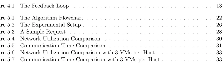
In order to solve the RSNAVMPP, I utilized a feedback design for implementation. A feedback loop, by definition, allows for reacting to changes caused by previous requests or external factors like workload fluctuation. A feedback design, along with an external input of the requests, allows for a solution to the RSNAVMPP to be implemented. In this chapter, I introduce the feedback design as it is used to solve the problem. This chapter then discusses the feasibility of such a design in data centers.
The above diagram depicts the different processes inside the feedback system and how they interact. Different processes that are components of the system are drawn in boxes. The entities that interact with these processes are labelled on the connectors like Actions and Monitored data. Other external factors that affect the system find a connector going into the system like Requests and Objectives.
The following is a detailed explanation of the feedback loop.
4.1
The External Inputs
The system takes in external parameters that are not defined or affected by the internals of the system. These can be user initiated or operator initiated. These entities are important in order to guide the system in a desired direction. There are two external inputs in the feedback loop that this study implements
Objectives
The objectives for the problem are fed to the system by the data center operator. Either of these objectives can be satisfied for the request depending upon the request. The choice of objective can be left to the user or the data center operator for each request. In the following chapters, for the sake of study, we have run experiments with either of the objectives. If the request asks to greedily minimize network utilization, then the problem becomes minimizing Equation 3.2. Likewise, if the data center operator chooses to give communication time a greater priority over network utilization, the problem becomes minimizing Equation 3.12.
Requests
As explained in the previous section, requests of virtual machines are dynamic. Their arrival is externally determined and not a product of any of the system’s functions, unless explicitly made to be. These requests are fed into the system, specifically to the Algo-rithm process which accepts the request and solves the RSNAVMPP. Each request can be accompanied by a choice of the objective piggybacked.
4.2
System under Management
The Actions suggested by the Algorithm are acted upon the data center. These actions result into the system changing its state. The system also undergoes changes from the data center administrator if the topology or the machines change. For the study, we will not consider these changes as external inputs to the system. We assume a fat tree topology.
The system is constantly monitored for two purposes. Firstly to understand the current state of the system. Secondly, to verify if the objectives are being met or not. The details about the monitoring activity is explained in the following section.
4.2.1 Algorithm
The Algorithm is brains of the system. The Algorithm component solves the real RSNAVMPP. It takes in requests for VM placment and gives out actions that suggest placement for the VMs requested. It also accesses the monitoring measurements made on the system while making the decision process.
The Algorithm serves each request one by one in a queue. This design assumes that multiple requests are not served by the algorithm concurrently. Even if multiple requests arrive at the Algorithm, a mechanism to sequentialize the requests is assumed to be in place. Handling multiple requests is not a part of the problem formulation. It is an implementation choice that is made in the study. Handling multiple requests is left as future work.
4.3
Monitoring and Measurements
Monitoring the system gives an accurate state of the system under management. The data gath-ered by monitoring helps the algorithm solve the RSNAVMPP in a reactive manner. Monitoring captures the changes brought about by a request or external factors like workload fluctuations and provides this data to the algorithm in its placement decision processing. This capter ex-plains monitoring and measurements in detail.
4.3.1 Variables to Monitor
The state of the system is represented by multiple parameters like per flow link utilization, machine CPU utilization, flow latency et cetera. Only certain parameters are useful for the algorithm in its decision making. Following are the parameters that are chosen for measurements in this study:
of physical disk space left. In this study, we limit the capacity to be determined by the cores in order to keep the implementation simple.
Link Utilization Each physical link has a limitation on the amount of traffic it can carry. The presence of a flow on the link is of crucial importance to the algorithm. If a VM is scheduled on a physical machine that is attached to a link that is already being utilized by a flow, that means the new VM’s flow will have to share the link. This leads to queuing delays. Hence, monitoring link utilization for presence of flows is crucial. The accurate percent of utilization is not used in this study to solve the RSNAVMPP.
4.3.2 Where and When to Monitor
Monitoring and measurements is a non-trivial decision to be made in this design methodology. An important decision is to decide the places from where to collect data in order to correctly estimate the desired parameters that comprise the state of the system. Moreover, the frequency of monitoring also determines the accuracy of the measurement.
Accuracy vs. Feasibility tradeoff
Monitoring has an overhead on the system [19]. For example, monitoring the amount of link utilization is done by looking at the port utilization on a switch port. Maintaining traffic statistics to a very granular level consumes CPU cycles for the switch. Various technologies like SFlow [8], Netflow [3] , IPFIX [9] and Openflow [17] exist that provide network utilization measurements. Each technology provides traffic measurements on a port upto certain level of accuracy and CPU overhead. For example, SFlow cannot provide an accuracy of nanoseconds to measure interpacket arrival times wheras it is possible with IPFIX to do that at an additional CPU overhead. There is an accuracy vs. feasibility tradeoff to take care of.
The actual monitoring details used during the experiments are given in the following sec-tions.
Maintaining Data Structures
Once a particular datum is collected, gathering it and storing it an intelligent fashion such that it becomes faster to access for the Algorithm component can decrease the overall complexity of the solution. Thus the data strucutres that hold the monitored data is a crucial part of the design.
the data could be arranged in a way that it reduces the lookup time for the algorithm. For example, in choosing the physical machine that has the highest amount of unused cores, if the data regarding the utilization of CPU cores is maintained in a descending array, the first element will always be the physical machine with the highest amount of unutilized CPU cores.
Distributing Calculation Complexity over Time
In the previous section we saw different representations of the state of the system. [18] have used a traffic matrix and a cost matrix that determines the cost for traffic to flow from one networking element to another. Both Meng et. al [18] and Daniel Dias et. al. [13] run their clustering calculations on the matrices everytime there is a change in the matrix. This leads to a lot of recalculation for those entities that have not changed state. Once this calculation is done, there is no calculation until the next pass. Instead of doing one big calculation every time, breaking that calculation over a period of time helps decrease the total complexity of the task.
Sorting a descending ordered array is a lot less compute intensive than clustering methods we saw in the previous efforts. Performing this less compute intensive sort for a large number of times, over a period of time gives the pipeline advantage of distributing tasks over a period of time.
4.4
Feasibility of Implementation of the Feedback Loop
Although the Feedback design is described in this section, here we attempt to justify our choice of this design to solve the RSNAVMPP.
The RSNAVMPP holds a lot of subtle characteristics like reactive, request specific and being network aware. The Feedback design helps to solve the problem in a reactive manner. The feedback design does not, by itself, provide any help in solving a request specific placement problem. But the feedback design does allow for a request specific processing of VM placements. Besides, the feedback design easily allows for maintaining of intelligent data structures.
The feedback design does not warrant any extra components or technology that is not al-ready existing in a data center. Modern data centers have practical uses for monitoring [16] . It could be traffic engineering, identifying workload shifts in order to manage resources, main-taining logs for official purposes and security. Hence, technology used for monitoring is an already existing part of the system. The transport of these measurements to the algorithm is an implementation detail.
Chapter 5
A Solution Algorithm
This chapter proposes a solution to the Request Specific Network Aware Virtual Machine Placement Problem. First, it presents the algorithmic solution to the problem. Then there is an explanation of the algorithm followed by Mathematical proof of greedy best solution. Following that, a few experiments are described that implement the algorithm which solves the RSNAVMPP.
5.1
Assumptions
The solution algorithm rests on a few critical assumptions:
The algorithm does not take into account location affinities of the application. For exam-ple, it is beneficial to schedule VMs that are going to access a lot of data to be placed close to their data source in order to decrease data fetch times. This affinity for certain places close to the data is called data locality [23]. Data locality is not accounted for in the algorithm. This means that any kind of bias brought in by the application that affects the placement of VMs is not incorporated into the Algorithm. Inculcating this bias into the feedback design means adding another external input to the system. Although data locality can be easily added as a bias into the algorithm, in order to keep the solution simple, it is left for future study.
The individual traffic patterns among VMs can be application / request sensitive [2]. Hence, these patterns are not explicitly used. If a flow is being recorded on a link, that link is assumed to be occupied by that flow although it might be giving only 10 percent of the time. Having multiple flows on a link is not discarded, it is discouraged.
before the request is deployed. Hence, all VMs within a request are assumed to commu-nicate with other VMs. Even if the VMs of the same request do not commucommu-nicate, they do not increase communication time or network utilization for that request, rather only decrease it. Hence, this assumption does not hurt the greedy lower bound of either of the objectives of the problem.
A Fat-tree topology is assumed for the rest of this study. Defining a topology helps determine the actual physical links and distances between physical machines. Most data centers operate on a fat tree topology or a close version of it [18]. Also, for the purposes of this study, the experiments assume a fat-tree topology not bigger than the aggregation layer. The algorithm transitions from the aggregation layer into a core layer exactly how it transitions from an access layer to the aggregation layer. Many topologies skip an aggregation layer and transition from access layer directly into core. The study assumes a two layer fat-tree topology.
5.2
The Solution Algorithm
In this section we describe a solution algorithm. The design enables a family of algorithms to exist. This study proposes the following algorithm as a solution to the RSNAVMPP.
The algorithm is based on three basic principles.
Sharing links
Sharing links means to have multiple flows belonging to different requests running on the same link. Having multiple flows on the same physical link leads to scheduling or queuing delays. This leads to an increase in the communication time for each of the flows running on the link. But the network utilization decreases because lesser links are used compared to having each flow separately on a link. In case of VMs on the same physical machine, sharing CPUs / memory / NIC will mean scheduling delays. In case of aggregation links being shared by flows,the queuing delays will increase as the number of flows sharing that link increases. It is critical to note that we do not take into account the actual traffic pattern in this study. Hence, we cannot comment into the actual percentage of sharing of the links. The mere presence of multiple flows is counted as sharing links.
Nearness of VMs
in terms of the number of physical link hops traversed to reach from one VM to another. Both network utilization as well as communication time for flows increases with distance between the VMs generating those flows. Reducing the number of hops will reduce the processing delays plus unnecessary utlization of network links.
The following is the pseudocode for the algorithm:
1: loop
2: when the previous request is done processing
3: if network utilization has priority over comm Time then
4: choose single physical server can contain the requested VMs.
5: if no single physical server has enough capacity then
6: choose least possible servers in one rack pocket.
7: if no single rack suffices then
8: select machines in one aggregation pocket that result into least number of links utilized.
9: if no single aggregation pocket suffices then 10: Hold the request for a random delay.
11: end if
12: end if
13: end if
14: else if comm Time has priority over network utilization then
15: choose single physical server can contain the requested VMs.
16: Preference to empty servers.
17: if no single machine sufficesthen
18: choose servers non-utilized links in a single rack.
19: if no single rack sufficient then
20: check for non-utilized links in an aggregation pocket.
21: using aggregation links and not sharing at access level will result into a smaller communication time.
22: if no single aggregation pocket has enough non-utilized links then
23: look for servers in one single rack, this time shared.
24: priority to servers will lease number of flows shared.
25: if no single shared access rack suffices then
26: use aggregation links with least shared links.
27: end if
28: end if
29: end if
31: end if
32: end loop
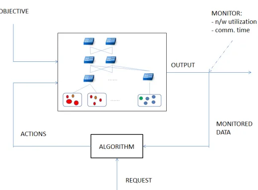
The algorithm first determines if the request has a higher priority for network utilization or communication time. Then the algorithm increases its spread across the topology by first checking if the requested VMs can be commissioned inside a single physical server. If not, the algorithm tries to commission them into one rack and then into one aggregation layer. In cases when communication time has a higher priority, greater stress is given on not sharing servers and links. Hence, when the communication time is a priority, those physical servers that do not have any other requests deployed and have sufficient capacity for all the requested VMs are chosen first for placing VMs. If not, then all the physical machines with sufficient capacity and connected to links that are not being used by flows of any other requests and are inside the same access layer pocket are checked for sufficiency. If these are not sufficient, a similar sufficiency check is made on the aggregation layer. In case the aggregation layer also does not have physical machines with sufficient capacity connected to empty links, we first resort to shared links at the aggregation layer. Here a critical distinction is between sharing links at aggregation layer and sharing links at access layer. Sharing links at aggregation layer is preferred as a fat tree topology has higher bandwidth links at the aggregation layer which help reduce queuing delays. In case sufficiently free physical machines are not found even then, the request is forced to wait until another previous request completes and its VMs are destroyed in order to create space.
The flowchart shown in Figure 5.1 describes the algorithm’s decision making process.
5.3
Mathematical Proof of Correctness
In this section we shall present the proof of greedy best placement achieved by the algorithm. The experiments detailed in the later section shall give a proof of concept of the same:
5.3.1 Mathematical Notations
Ji : A request that generate flows (f1, f2, ..., fm) and utilize Links (L1, L2, ..., Ln) of
band-width (B1, B2, ..., Bn) during the time 0→T.
At any point in time, (J1, J2, ..., Ji−1) are deployed in the data center.
Jidui
t : Bytes transferred by fi at the tth time interval belonging to request Ji. These
Figure 5.1: The Algorithm Flowchart ‘
5.3.2 Proof for greedy objective Network Utilization
The algorithm chooses different paths of operation depending on the priority of objectives as specified by the user. A single request cannot claim equal priority for both the objectives. We proove that the algorithm chooses the greedy best placement for both the objectives one by one.
First, let us proove for communication time. Our Aim is to find physical machines which when deploy the VMs requested by a new requestJi result into the least communication time
for that request.
The fastest way to communicate is not use the network at all. Hence, Bj is the highest
as compared to any physical link andn= 0. Hence, we seek to find one physical machine with enough capacity to host all the VMs requested.
In case of empty machines, m= 0.
Ti= 0
X
j=1
Di∗pk
Bj
+
D
X
p=1 0
X
j=1
P0
i=1pi∗Di
Bj−1
= 0 (5.1)
of delay in scheduling as the VMs share processor with other VMs.
m≤maximum capacity of VMs that a machine can host (5.2)
Bjinside the machine transfer>> Bjon the network (5.3)
Ti = 0
X
j=1
Di∗pi
Bj + D X p=1 0 X j=1 Pm
i=1pi∗Di
Bj−1
= 0 (5.4)
Next, we try to minimize m by keeping m = 0. As the switch will always have packet memory shared with other flows, there might be some queueing delay in this case. Keeping all VMs confined to one rack pocket will result into n= 2 and a constant Bj as the link
bandwidth at access layer levels we assume is the same. This is true irrespective of the number of physical machines or links we use. Hence, we try to minimizem again. Using only non-utilized links - data gathered by monitoring, we getm= 0.
iTi = 2
X
j=1
Di∗pi
Baccess + D X p=1 1 X j=1 P0
i=1pi∗Di
Baccess
(5.5)
iTi = 2
X
j=1
Di∗pi
Baccess + D X p=1 1 X j=1 P0
i=1pi∗Di
Baccess
(5.6)
If, no single rack has enough capacity to hold machines, we move to one aggregation pocket. Now, we choose those machines that result into links not getting shared at access level. Links at aggregation level are fatter and hence, if provisioned correctly, sharing links at aggregation level does not result into reduction of time.
5.3.3 Proof of greedy objective Network Utilization Next, we proove the network utilization greedy objective is achieved.
First, we check for one machine. If all the requested VMs are deployed in a single physical machine, n= 0.
utilization(Ji) = m X i=1 0 X j=1 Tf X
t=Ti
Jidui
t= m
X
i=1
If that does not work, we try to accomodate all the VMs requested in a single rack. This is because thenn= 2 for each flow.
utilization(Ji) = m X i=1 2× Tf X
t=Ti
Jidui
t (5.8)
Next, we try for one aggregation layer pocket. Here n= 4.
utilization(Ji) = m X i=1 4× Tf X
t=Ti
Jidui
t (5.9)
5.4
Complexity Calculations
The overall complexity of the algorithm is divided in two parts. The computation to be done to solve the algorithm itself and the computation done to maintain the data structures.
5.4.1 Complexity of Maintaining Data Structures
Let us first gain a greater understanding of the data structures involved. That will make cal-culating the complexity easier. Following are the data structures that were used in this study:
CapacityArray- For each rack, maintain a descending sorted array of leftover capacities in physical servers. There arem such arrays ofn elements each signifyingm total access layer switches and nhosts connected to each of those switches.
GlobalCapacityArray - One global descending sorted array containing the sum of Ca-pacityArrays for each access layer switch i.e. the sum of leftover capacities of physical machines connected to each access layer switch. There is one such array containing m
elements for each access switch.
LinkUtilArray - For each rack, maintain an ascending sorted array of link utilization. i.e. number of flows on the link. There arem such arrays of nelements.
Everytime monitored data is brought in to the data structure, the array needs to do a binary search for the proper place of the updated value of the capacity. This takes O(logn∗K) time whereK is the monitoring frequency of data. K is an implementation detail.
The sum of a CapacityArray represents the amount of capacity left in one access layer pocket. Hence, each time a datum is updated, in addition to sorting the respective Capacity Array, the GlobalCapacityArray must be updated to the sum of the respective Capacity Array and sorted in descending order. This takes the updating cost toO(logm∗K) because updating the sum is a constant time operation wheras placing the new value in its proper sorted position requires a binary sort on GlobalCapacityArray.
The LinkUtilArray maintains an ascending sorted array of the Link Utilization for each link in a rack, for all racks. The array records the presence of flows on the links. Sorting this array takes O(logn).
Hence, the total cost of maintaining the structures is:O(n∗logn) +O(logm∗K) +O(logn). 5.4.2 The Algorithm Complexity
The algorithm reads data from the data structures, does some processing and gives out results. Most of the complexity involved is in getting access to the data in the correct form. The algorithm takes two separate forks for the two objectives.
Complexity for Network Utilizatoin
Checking if a single physical server can contain all the requests is done in O(m) time as the first elements of the each of the CapacityArrays is scanned. If a physical machine suffices, our request is placed on this physical machine. If it is not, none of the physical servers have enough capacity to host this request. We will then try to place the request inside one access layer pocket.
Checking if one access layer switch contain all the VMs requested takes O(1) time as the first element has the maximum capacity. If that rack does not suffice, none of the others will.
Checking for an aggregation layer pocket to contain all the VMs requested takes O(m) amount of time to sum the capacities of access pockets forming an aggregation pocket.
Hence, the worst case complexity for a request that chooses to optimize network utilization isO(m).
Complexity for Communication Time
worst case. Similarly, if the request reaches upto the aggregation layer, the worst case complexity reaches uptoO(m∗n).
Hence, the worst case complexity for Communication Time is O(m∗n).
The overall complexity of the solution algorithm is the summation of the worst case com-plexities of the algorithm itself and the complexity of maintaining data structures:O(m∗n) +
O(n∗logn) +O(logm∗K) +O(logn)
5.5
Experimental Results
In the previous sections, we suggested a solution and proved its correctness. In order to show-case a proof of concept, certain experiments were conducted with test show-cases. This section will highlight the experimental setup, the expected results, the results obtained and experience of conducting the experiments.
5.5.1 The Setup
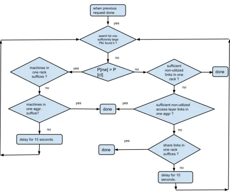
The experiments were conducted in a small setup, powerful enough to have a proof of concept implementation of the solution. The setup is depicted below:
Hardware
The setup consists of six off-the-shelf physical machines and three Extreme Newtorks Summit X440 switches [4] . The switches and physical machines are arranged in the topology shown. There is a management switch (not shown) that connects to all the switches and the physical machines, used to ssh. The diagram shows the production network. Each link in the diagram is a 1Gbps link.
Each Physical Machine is an off-the-shelf IBM Machine containing 2 Cores, 3 GB of RAM and 180 GB of disk space. Each machine runs the server version of Ubuntu 12.04. The Physical Machines are not very powerful and the experience section later details the limitations faced due to these.
Software
Following are the software components used in this study:
Openstack [7] was used as an orchestrating software for creating VMs, deleting VMs. Openstack is an open source virtualization orchestration software and has a vibrant com-munity that was very helpful in the steep learning curve phase for the author. The Havana version of Openstack was used in this study. The Openstack Nova controller ran on Fire machine.
Iperf [5] was used to generate user traffic. Iperf is the most basic traffic generator that was used to generate TCP flows between VMs. Iperf provides with excellent measurements of time taken to complete the flows that were used in traffic generation. These measurements were used to report the flow time in this study.
Openflow [17] was used to collect measurements. The Opendaylight Project [6] was used as an openflow controller. Opendaylight is an opensource software developed by an industry consortium of the same name. The opendaylight community was a big help in learning the controller. The opendaylight controller ran on Water machine labelled in the diagram.
The Algorithm itself ran on Fire along with the Openstack Nova controller. The open-daylight controller ran on the Water machine. That meant 4 physical machines were used as hosts in the topology shown in the diagram.
5.5.2 Parameters of Interest
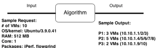
Each request asks for certain number of VMs and of certain type.
Figure 5.3: A Sample Request
Following are some of the parameters that are of interest while running experiments: Virtual Machine TypeEach VM request may vary in its requirement of CPU Cores,
RAM and disk requirements. In a public cloud, the user chooses the configuration of the VMs he/she desires. For a private data center, the request may depend upon the application that will run on those VMs. For this study, we consider a constant VM type for all the requests. Each VM has 1 virtual CPU, 512 MB RAM and 10 GB of disk space. The reasons and feasibility of this decision is explained in Section 5.5.4
Number of VMs per Request Each Request requires a certain number of VMs. This is a very crucial parameter that has been explored in the experiments.
Topology The topology of a data center will bring a radical change in the behavior of the algorithm. Although the solution assumes a fat-tree topology, but the exact number of physical machines on switches, the size of the links et cetera greatly impact the output of the algorithm. For the sake of this study, the topology is kept constant at that shown in the diagram. Again, the reasoning behind this choice is explained in the experimental limitation sections.
Traffic The VMs in the experiments exchange certain traffic. The amount of traffic ex-changed has a major impact on the communication time in an absolute manner. But the traffic profile is kept to be a constant TCP flow transferring 120 GB of data from one VM to another throughout the experiments. As assumed in the solution, the exact nature of the traffic is not considered in this study. Hence, any choice of traffic is a valid one. The constant TCP transfer was used with Iperf due to its simplicity and experience of the author with that tool.
Transport of Monitored Data The Algorithm and Nova controller run on the same machine. Hence, transfer of data is done in-memory. The Opendaylight controller runs on a separate machine. This is because of limitation on the number of NICs on a single machine. The amount of time taken to transport the monitor data can also impact the experiments. In such a low profile setup this parameter is not explored. But otherwise, the accuracy vs. feasibility tradeoff of monitoring and measurements becomes crucial. Hypervisor choiceThis is one parameter that was found out to profoundly impact the
results of experiments. Hypervisors perform differently in the areas of compute, network I/O and disk I/O [12]. A hypervisor like KVM that is a full hypervisor has better compute and network I/O than QEMU which is an emulation software. This topic is further explored in the experimental limitations section.
5.5.3 Results
Following are the experiments that explore the algorithm and show some its advantages:
Experimenting with Objectives
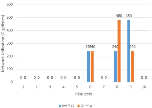
The RSNAVMPP outlines two objectives that need to be achieved for each request in an either or fashion. The algorithm takes in 10 requests for VMs in the order: [3,2,3,1,4,8,1,7,10,2]. This is a sequence of the number of VMs demanded by each request. The configuration of each VM is 512 MB RAM, 1 Virtual CPU and 10 GB disk space. Two runs of the experiment were conducted. One with the objective being to minimize network utilization and the other being with the objective of minimizing communication time.
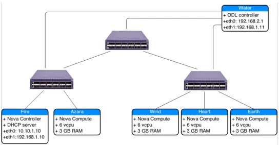
The network utilization resulting from the traffic exchanged by VMs placed is shown in Figure 5.4. For each request, the network utilization observed in both cases, one, when network utilization is a priority and second, when communication time is a priority.
Figure 5.4: Network Utilization Comparison
high, if not zero. This is attributed to the fact that the setup is very minimal and is not able to capture the utilization at a true granularity. The utilization is a multiple of 120GB, the amount of data transferred by each flow. Total number of links in the whole setup is 6 and hence, we obtain a weak result here.
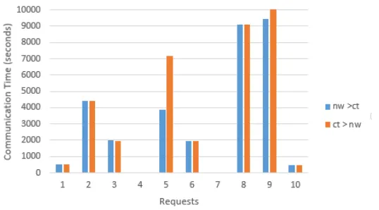
In Figure 5.5, the Communication Time for each request resulting from the VMs placed as per requests is shown. Same as before, the communication time in both cases, one, when network utilization is a priority and second, when communication time is a priority is shown.
Communication time has a higher granularity here. For most of the requests, the commu-nication time is lesser when the request chose to prioritize commucommu-nication time over network utilization as its objective. The communication time for request 7 though is an anomalous. This request was hosted primarily on Earth, which runs on QEMU, and shows lower performance when over commissioned. Otherwise, in general, the algorithm performs well to decrease the communication time relatively.
Experimenting with Request Sequence
Among the parameters of interest, the Request Sequence is also an important parameter to the solution. The Request Sequence is the order in which requests arrive to the algorithm. This test case considers two different request sequences and observes the difference in network utilization and communication time attained.
The two requests are as following:
Figure 5.5: Communication Time Comparison
Larger Requests: 7,4,2,8,3,10,4,2,5,7 - This sequence has higher number of VMs re-quested. This sequence acts in a way contradictory to the previous sequence as this one fulfills all the servers in the beginning and thus the later requests must wait for the former ones to complete before enough space can be created. The maximum number of VMs that can operate at one time is 24.
The communication times obtained are compared in Table 5.1 and the network utilization measurements obtained in the experiments are compared in Table 5.2.
Table 5.1: Comparing Communication Time for both sequences. Larger sequence on the right.
The ones on the right are measurements for the larger sequence.
Table 5.2: Comparing Network Utilization for both sequences. Larger sequence on the right.
requests, the algorithm is able to schedule them without sharing as each request has to wait for the previous request to complete. The setup being small will not be able to sustain too many requests for VMs at one point.
We also notice that the anomalous behavior in all the graphs comes from the request that demands 8 or 10 VMs. This is so because the physical machines are already over commissioned and putting extra workload on them creates CPU delays that are not inherent to the algorithm. We discuss this problem of over commissioning in detail. Also, these requests are deployed on the machine Earth again.
Experiments with Physical Machine Capacity
In this set of experiments, we vary the maximum capacity of the Physical Machines from 6 to 3. The reduced physical capacity means each physical machine will not host more than 3 machines at one time. The maximum number of total VMs in the setup at one time becomes 12. This is a very small number. This set of experiments will showcase the effect of having too weak a setup.
Figure 5.6 and in Figure 5.7 show that the change in objectives do not cause a major change in the performance of the algorithm when the physical capacity of the host is reduced. The network utilization is the exact same irregardless of the objective. Wheras, the Communication Time is same at most places and even worse at Request number 7. The reduction in capacity means that the sample size has reduced too low to make any legit comments on the outcome.
5.5.4 Experimental Limitations and Experience
Figure 5.6: Network Utilization Comparison with 3 VMs per Host
experience of conducting the experiments.
6 VMs on 1 Physical Machine:The machines used in the experiments are off-the-shelf machines with cheap configurations. Each machine has only 2 cores. The default ratio for Openstack is to have 1 CPU become 1 Virtual CPU (vCPU) for the VMs. But then each machine would host 2 VMs and in total only 8 VMs are hosted. Hence, the author over commissioned the CPU’s making the CPU:vCPU ratio = 1:4. Now, each CPU is shared between 4 VMs. In total 8 VMs can run on a single physical machine. Overloading the machines causes skewed results. Predictable results are important in order to verify the behavior of the algorithms. Hence, each physical machine is limited to running 6 VMs at maximum.
10 Requests in a Sequence:For most of the experiments, there are 10 Requests within a request sequence. Having lesser number of requests results into too low sample space to prove any substantial behavior of the Algorithm. More than 10 Requests results into uncommonly large experiment times.
Experiment TimesWith 10 Requests in a sequence, each experiment runs over 6 hours average for one objective. In a single experiment, more than 60 VMs are created and destroyed. The low end machines suffer a high overhead in creating and deleting VMs. Also, not all experiments are completed successfully. An additional nuisance was VMs crashing more than half way through the experiment. This lead to a restart of the whole experiment.
120 GBytes of Traffic transfer:The traffic that is transferred has a very big impact on the experiment time. After much experimentation, 120GBytes of constant transfer via TCP was the traffic pattern used. Iperf’s UDP traffic generation slowed down considerably, sometimes reaching 2 Mbps rates, when the physical machines neared the end of their capacity. Hence UDP is not used. There aren−1 flows generated by a request fornVMs. Choosing anything lesser than 100Gbytes of TCP transfer per flow makes the request very short lived; too small to be create a realistic data center scenario. TCP transfers above 150GBytes lead to very high experiment times.
1 Gbps Links: All the links shown in the setup are 1 Gbps links. Ideally the aggregation links are higher in bandwidth than the access layer links. But 10G NICs were not available. 100 Mbps links are not used as the traffic transferred over 100 Mbps links as 100 Mbps links are rarely used in data centers and hence does not warrant good measurements. Single VM Image: A single VM image type was used throughout the experiments.
space. Openstack does not allow a VM image to have lesser than 512 MB RAM and 1 vCPU. Having higher configuration for a single VM led to less number of VMs per physical machine. The chosen configuration led to 6 VMs per machine and 24 VMs in total. Any higher configuration led to unfeasibile scenarios.
Chapter 6
Conclusion and Future Work
This chapter tries to conclude the study and summarize the major findings. It also outlines limitations of the study and future work.
6.1
Reactive Placements and Customizable Objectives
A Google data center that runs indexing jobs for the web, has completely different resource management objectives than an Amazon one. A solution to the Virtual Machine Placement problem should attempt to solve the VMPP for both Google as well as Amazon. Being able to solve a problem reactively allows the solution provided in this study to customize objectives according to the objective requirements of the data center.
The results showcase the use of Openstack for such experiments. Besides, this study makes a convincing case to adopt better scheduling techniques inside Openstack nova.
6.2
Limitations and Future Work
Processing Multiple Requests
In this study, the algorithm assumes a mechanism for limiting the arrival of requests to one at a time. This leads to a sequence of requests going as input to the algorithm. But that is not a limitation of the design or the problem. Handling multiple requests together in order to achieve greedy objectives is possible. This is left for future work.
Location Affinity and Incremental Requests
can be accmmodated in the solution in a greedy manner. Instead of picking the best placement out of all, the best placement closest to the affable location will lead to a greedy solution that accommodates location affinity.
Incremental requests for VM placement are essentially requests for addition of VMs to al-ready deployed requests. This poses the same challenge as location affinity under the assumption that VMs of the same request will communicate.
Other Topologies
This study assumes a Fat tree topology. But the RSNAVMPP does not specify the topology. A solution that works for topologies other than the Fattree like VL2 and Clos will add value. A complete solution would be topology agnostic.
Non Greedy Objectives
Here the RSNAVMPP is limited to greedy optimization objectives. We leave it to future work to present a problem spanning non-greedy objectives and find a solution to the same.
Traffic Agnostic
REFERENCES
[1] AmazonEC2. http://aws.amazon.com/ec2/, Accessed: 2014-06-30.
[2] Big Data in the Enterprise - Network Design Considerations White Paper. http://www. cisco.com/c/en/us/products/collateral/switches/nexus-5000-series-switches/
white_paper_c11-690561.html, Accessed: 2014-06-30.
[3] Cisco Systems NetFlow Services Export Version 9. http://www.ietf.org/rfc/rfc3954. txt, Accessed: 2014-06-30.
[4] Extreme Networks Summit X440. http://www.extremenetworks.com/product/ summit-x440-series/, Accessed: 2014-06-30.
[5] Iperf - The TCP/UDP Bandwidth Measurement Tool.http://iperf.fr/, Accessed: 2014-06-30.
[6] Opendaylight - A Linux Foundation Collaborative Project. http://www.opendaylight. org/, Accessed: 2014-06-30.
[7] Openstack - Open Source Cloud Computing Software. https://www.openstack.org/, Accessed: 2014-06-30.
[8] SFow. http://www.sflow.org/, Accessed: 2014-06-30.
[9] Specification of the IP Flow Information Export (IPFIX) Protocol for the Exchange of IP Traffic Flow Information. http://tools.ietf.org/html/rfc5101, Accessed: 2014-06-30.
[10] Hitesh Ballani, Paolo Costa, Thomas Karagiannis, and Ant Rowstron. Towards predictable datacenter networks. ACM SIGCOMM, August 2011.
[12] Jianhua Che, Qinming He, Qinghua Gao, and Dawei Huang. Performance measuring and comparing of virtual machine monitors. In Embedded and Ubiquitous Computing, 2008. EUC ’08. IEEE/IFIP International Conference on, volume 2, pages 381–386, Dec 2008.
[13] D.S. Dias and L.H.M.K. Costa. Online traffic-aware virtual machine placement in data center networks. InGlobal Information Infrastructure and Networking Symposium (GIIS), 2012, pages 1–8, Dec 2012.
[14] Derek Gottfrid. Self-Service, Prorated Supercomputing Fun! http://open.blogs. nytimes.com/2007/11/01/self-service-prorated-super-computing-fun/?_php=
true&_type=blogs&_r=0, Accessed: 2014-06-30.
[15] Chris Hyser, Bret Mckee, Rob Gardner, and Brian J Watson. Autonomic virtual machine placement in the data center. Hewlett Packard Laboratories, Tech. Rep. HPL-2007-189, pages 2007–189, 2007.
[16] Lavanya Jose, Minlan Yu, and Jennifer Rexford. Online measurement of large traffic aggregates on commodity switches.
[17] Nick McKeown, Tom Anderson, Hari Balakrishnan, Guru Parulkar, Larry Peterson, Jen-nifer Rexford, Scott Shenker, and Jonathan Turner. Openflow: enabling innovation in campus networks.ACM SIGCOMM Computer Communication Review, 38(2):69–74, 2008.
[18] Xiaoqiao Meng, Vasileios Pappas, and Li Zhang. Improving the scalability of data center networks with traffic-aware virtual machine placement. In INFOCOM, 2010 Proceedings IEEE, pages 1–9, March 2010.
[19] Andrew Moore, James Hall, Christian Kreibich, Euan Harris, and Ian Pratt. Architecture of a network monitor.
[21] Fei Song, Daochao Huang, Huachun Zhou, and Ilsun You. Application-aware virtual ma-chine placement in data centers. InInnovative Mobile and Internet Services in Ubiquitous Computing (IMIS), 2012 Sixth International Conference on, pages 191–196, July 2012.
[22] Chunqiang Tang, Malgorzata Steinder, Michael Spreitzer, and Giovanni Pacifici. A scalable application placement controller for enterprise data centers. In Proceedings of the 16th international conference on World Wide Web, pages 331–340. ACM, 2007.