Hand Movement Classification using Burg Reflection
Coefficients
Daniel Ramírez-Martínez1, Mariel Alfaro-Ponce2 , Oleksiy Pogrebnyak1,‡ , Mario Aldape-Pérez3 and Amadeo-José Argüelles-Cruz1,∗
1 Centro de Investigación en Computación, Instituto Politécnico Nacional. Av."Juan de Dios Bátiz" s/n esq.
Miguel Othón de Mendizábal, Col. Nueva Industrial Vallejo, Del. Gustavo A. Madero, Ciudad de México; [email protected]; [email protected]; [email protected]
2 Departamento de Ciencias e Ingenierías, Universidad Iberoamericana Puebla. Blvrd del Niño Poblano 2901,
Reserva Territorial Atlixcáyotl, Centro Comercial Puebla, 72810 San Andrés Cholula, Pue. México; [email protected]
3 Centro de Innovación y Desarrollo Tecnológico en Cómputo, Av."Juan de Dios Bátiz" s/n esq. Miguel Othón
de Mendizábal, Col. Nueva Industrial Vallejo, Del. Gustavo A. Madero, Ciudad de México, C.P. 07700.; [email protected]
* Correspondence: [email protected]; Tel.: +52-55-5729-6000 ext.56593
∥ ‡In Memoriam
Version October 29, 2018 submitted to Preprints
Abstract:Classification of electromyographic signals has a wide range of applications, from clinical 1
diagnosis of different muscular diseases to biomedical engineering, where their use as input control 2
of prosthetic devices has become a hot topic of research. Challenge of classifying this signals relies 3
on the accuracy of the proposed algorithm and the possibility of its implementation on hardware. 4
This paper consider the problem of electromyography signal classification, solved with the proposed 5
signal processing and feature extraction stages, with focus lying on the signal model and time domain 6
characteristics for better classification accuracy. The proposal considers a simple preprocessing 7
technique that produces signals suitable for feature extraction, and the Burg reflection coefficients to 8
form learning and classification patterns. These coefficients yield a competitive classification rate 9
compared to used time domain features. Sometimes, the feature extraction from electromyographic 10
signals showed that procedure can omit less useful traits for machine learning models. Using feature 11
selection algorithms provides a higher classification performance with as fewer traits as possible. 12
Algorithms achieved a high classification rate up to 100% with low pattern dimensionality, with other 13
kinds of uncorrelated attributes for hand movement identification. 14
Keywords:Electromyography, Hand Movement, Health Monitoring, Maximum Entropy Reflection 15
Coefficients, Classification Algorithms, Machine Learning, Feature Selection. 16
1. Introduction 17
Electromyography (EMG) is an electrodiagnostic medical procedure to assess the health of muscles 18
and the nerves cells that controls them, with the detection, recording and analysis of electromyography 19
signals (sEMG). The EMG provide physicians and health experts with the information generated by 20
the muscle contractions, that is the ionic flow through the muscle fibre [1]. Research has considered 21
EMGs as an important field of study due to the diversity of its applications in clinical medicine and 22
biomedical engineering [2]. EMG has applications such as the diagnosis of nervous system disorders 23
and muscular diseases like myopathies detection and neuropathies [3–5]. All these applications need 24
preprocessing of signals and its extraction of features [6]. sEMG are useful as input control signals for 25
prosthetic limbs [7,8], in rehabilitation as a measurement parameter of muscular effort [9], and for the 26
development of muscle machine interfaces [10]. 27
Most EMG applications involves real-time systems, that are needed to run with low-cost 28
computational features [11]. As a matter of the fact, in the development of prosthetic, orthotic and 29
rehabilitation devices the EMG can be employed as a part of the control system. In the results reported 30
by [12] EMG pattern recognition and myoelectric control are compared for prosthetic control, the 31
paper remarks that these signals are suitable for the control with highlights in the implementations of 32
algorithms that are capable to distinguish between signals that have similarities. These similarities are 33
presented in users that have lost a body part, as a consequence of the absence of peripheral structures 34
in the musculoskeletal system, where the classification of EMGs features become a challenge. The 35
most used EMGs features are time domain attributes [13] that can be obtain by root-mean-square 36
value (RMS), mean average value (MAV), variance (VAR), Willison amplitude (WAMP), wavelength 37
(WL), and many others [14] [15]. These characteristics have been used in different classification tasks, 38
and the classification rate increases with the use of a proper signal preprocessing stage; for instance, 39
Chowdhury et al. consider the use of wavelet and empirical mode decomposition, first differentiation 40
or independent component analysis in [15]. Despite the performances achieved at the preprocessing 41
stage, computational complexity might increase adding a delayed response. Several authors use 42
autoregressive models and the characteristics of random processes, such as first and second moments 43
and others, in tasks related with classification of myopathy or neuropathy diseases. For example, 44
Bozkurt et al. report 97% in performance using fifteenth order autoregressive models (AR) Yule-Walker, 45
Burg, Covariance, Modified Covariance and subspace base methods to extract features from 1200 46
sEMG, applying high resolution and high sampling rate in invasive electrodes implanted in a Bicep 47
brachii muscle [16]. 48
In a different research dedicated to the hand movement, Phinyomark et al. report a high 49
classification rate of 97.76%, achieved by applying a quadratic discriminant analysis and four AR 50
coefficients per channel and including a preprocessing stage whose output is the first differentiation 51
of sEMG [17]. They extracted information from the activity of five forearm muscles: WL, difference 52
absolute mean value (DAMV), difference absolute standard deviation value (DASDV), difference 53
absolute variance (DVARV), difference absolute standard deviation (DASDV), second order moment 54
(M2), WAMP, integrated EMG (IEMG), MAV. They used also these features in their previews works [18]. 55
Simple squared integration SSI, VAR, RMS, myopulse percentage rate (MYOP), cepstral coefficients 56
(CC), log detector (LOG), temporal moment (TK) and v order (V) with another point of view in [17] 57
applying the seventh order Daubechies mother wavelet and the four decomposition levels before 58
sEMG characterisation extracts RMS and MAV. They test the behaviour of these traits to estimate 59
whether they are useful for identification of six daily hand movements monitoring flexor and extensor 60
carpi radialis longus muscles. 61
Liu et al. describe the use of an assemble classifier of support vector machines (SVM) [19], 62
classifying eight different hand grasps with a precision rate of 93.54%; extracting sEMG from three 63
different forearm muscles and fourth order AR coefficients and HEMG builds the feature vector per 64
channel. In their work the aim is to get significant features and a classification model that permits 65
increasing the classification rate of sEMG. However, assembling SVM models results computationally 66
expensive. Angari et al. consider fifteen channels to digitalise sEMG and to characterise five hand 67
movements, where they extract twenty-one attributes per channel (MAV, WL, ZC, SSC, AR6, and 68
others) to implement feature selection methods and channel discrimination [20]. In this case, the aim 69
of the research was to train the SVM with low dimensionality patterns and the most representative 70
forearm muscles; this work concludes that MAV and WL are appropriative for classification tasks. 71
The method of Khezri et al. uses an adaptive neuro–fuzzy inference system to test its classification 72
rate in a six hand movement dataset containing four channels [21]. The considered features are MAV, 73
SSC, ZC, and 10 order AR model coefficients. Merging these attributes to create patterns for sEMG 74
representation provokes that classification rates runs from 86% to 100%. 75
Ruangpaisarn et al. present a feature extraction technique for hand movement classification, 76
considering two pairs of EMG electrodes and the merging and transformation of both channels 77
into a squared matrix to perform factorisation via singular value decomposition [22]. They report 78
instances, achieving a performance of 98.22%. The issue in this work comprises taking samples where 80
no muscular activity is looked at, and working with a 2D vector in most cases leads to non-linear 81
computational complexity. With the same dataset, Sapsanis et al. used a preprocessing stage in which 82
signals are 3 level decomposed with empirical mode decomposition, so that noise is reduced [23]. 83
For each decomposition level and raw sEMG, they extract the following attributes: IEMG, ZC, VAR, 84
SSC, WL, WAMP, kurtosis and skewness. With a linear discrimination analysis, a rate of correct 85
classifications reaches 89.21%. 86
The resumes in [14] and [15] show the variety of features for classifying sEMG and preprocessing 87
techniques that might lead to a classification model performance increasing. However, none of the 88
studies use the reflection coefficients as features for pattern recognition. 89
The aim of this work is to develop a classification algorithm for sEMG with low computational 90
cost and with a competitive classification rate. The remainder of this paper present the following 91
distribution: Section2describe the hand movement database that was employed, also a brief resume 92
of the signal preprocessing techniques and different features useful for classification are described. 93
Then, the proposed classification method is presented. Section3shows the results obtained by the 94
classification technique. Section4and5are the discussion and conclusion of the results achieved by 95
the proposed methodology for sEMG classification. 96
2. Materials and Methods 97
2.1. Data selection and preprocessing 98
We used an EMG dataset from the University of California in Irving (UCI) machine learning 99
repository, the same as in [22] and [23]. The data describes six different hand movements taken from 100
Flexor Capri Ulnaris and Extensor Capri Radialis muscles of five healthy people (three women and 101
two men) who performed with no restrictions thirty times each hand action during 6 seconds each; 102
signal sampling frequency is 500Hz. The dataset contains 1800 time series available to classify 6 hand 103
grasps (Spherical, Tip, Palmar, Lateral, Cylindrical and Hook). 104
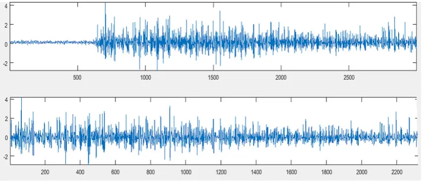
Before feature extraction, there is a simple preprocessing treatment applied to each signal. At 105
the first preprocessing stage, the method eliminate the initial samples, where muscle activation is 106
absent and only noise is present, to avoid the feature extraction lacking the phenomena information. 107
The next step comprises the extract of the signal-mean-value at all data points; this operation 108
is important to comply with the restrictions imposed by the optimal linear filtering theory [24]. 109
Linear prediction model framework requires restrictions such as autoregressive models. Otherwise, 110
performing classification/prediction models might decrease. Here, we used the simple arithmetic 111
mean value computed as 112
x= 1
N N
∑
n=0
x[n] (1)
wherex is the mean value; x[n] is EMG signal and N is the total number of samples. The 113
application of the mean (1) implies a new sample value which is described asx[n] = x[n] −x for 114
1≤n≤N. Figure1illustrates the proposed preprocessing stages. 115
These two conditioning steps have linear complexity and supply feature extraction stage with an 116
appropriated sEMG. 117
2.2. Standard time domain features 118
The integrated EMG feature is defined as the cumulative addition of each signal sample absolute 119
value: 120
IEMG=
N
∑
n=0
Figure 1.On top original signal, on bottom clipped signal with zero mean value.
where other attribute is mean absolute value; it is one of the most useful attributes in many researches and consists of computing the mean absolute amplitude value of sEMG:
MAV= 1
N N
∑
n=0
∣xn∣ (3)
The simple squared integration feature describes the energy of sEMG and is mathematically 121
defined as cumulative addition of absolute squared value of each sample: 122
SSI=
N
∑
n=1
∣xn∣2 (4)
A stochastic process as a sEMG can be defined by its first and second order moment, i.e., mean and 123
variance values. Therefore, these features might be part of the pattern. The mathematical definition for 124
the variance takes considers a sEMG is a near to zero mean process, so its definition becomes: 125
VAR= 1
N−1
N
∑
n=1
xn2 (5)
The root mean squared value (RMS) reveals the information of the amount of strength yield by a 126
muscle, and is defined as the square root of the mean squared values. In many research works, this 127
attribute is considered important for different tasks: 128
RMS= ¿ Á Á
À1
N N
∑
n=1
xn2 (6)
The wave length is a distance between a pair of adjacent samples along all sEMG: 129
W L=
N
∑
n=1
∣xn+1−xn∣ (7)
The zero crossing feature describes the number of times that the sEMG amplitude becomes 130
positive or negative. Its definition considers a threshold whose aim is to count only the events 131
produced by muscular activity: 132
ZC=
N−1
∑
n=1
[sgn(xn×xn+1) ⋂ ∣xn−xn+1∣ ≥0],sgn(x) = {1, x
≥threshold
The slope sign attribute considers three adjacent samples to determine the number of times that a 133
slope sign between these sEMG values changes: 134
SSC=
N
∑
n=2
f((xn−xn−1) × (xn−xn+1)),f(x) = {1, f =th
0, otherwise (9)
wherethis a threshold. 135
The quantity of motor unit action potential is estimated through the Willison amplitude counting 136
the number of times that two adjacent samples overcome a threshold reducing artifacts produced by 137
noise: 138
WAMP= 1
N N
∑
n=1
f(∣xn∣),f(x) = {1, x ≥th
0, otherwise (10)
The amount of muscular pulses is described by the log detector which uses a threshold to avoid 139
noisy samples. 140
MYOP= 1
N N
∑
n=1
f(∣xn∣),f(x) = {1, x ≥th
0, otherwise (11)
2.3. Autoregressive model features 141
A linear autoregressive model describes a random process usingpcoefficients [24]. The goal 142
consists in extractingpcoefficients to construct a representation of each sEMG samplex[n]with the 143
preceding signal values(x[n−1],x[n−2],. . . ,x[n−p])making a linear combination, which carries an 144
error or white noise term: 145
x[n] =
p
∑
k=1
akx[n−k] +e[n] (12)
wherex[n]is the generated sEMG value throughkearlier samplesx[n−k],pis the order of the 146
model,e[n]expresses an added error or white noise term andakis the autoregressive coefficients. The 147
mathematical approach used to derive the autoregressive coefficients defines the regressive model 148
type. The most popular autoregressive model is the Yule-Walker model that uses the estimated values 149
of the correlation function calculated as: 150
ˆ
rxx(n,n−k) =Ex(n)x(n−k)k=0,±1,±2, ... (13)
Having ˆrxxestimated with (13), aNxNsquared Yule-Walker matrix equation is built as follows: 151 ⎡ ⎢ ⎢ ⎢ ⎢ ⎢ ⎢ ⎢ ⎢ ⎣ ˆ
rxx(0) rxxˆ (−1) ⋯ rxxˆ (−p)
ˆ
rxx(1) rxxˆ (0) ⋯ ˆrxx(−p+1)
⋮ ⋮ ⋯ ⋮
ˆ
rxx(p) rxxˆ (p−1) ⋮ rxxˆ (0) ⎤ ⎥ ⎥ ⎥ ⎥ ⎥ ⎥ ⎥ ⎥ ⎦ ⎡ ⎢ ⎢ ⎢ ⎢ ⎢ ⎢ ⎢ ⎢ ⎣ 1 a1 ⋮ ap ⎤ ⎥ ⎥ ⎥ ⎥ ⎥ ⎥ ⎥ ⎥ ⎦ = ⎡ ⎢ ⎢ ⎢ ⎢ ⎢ ⎢ ⎢ ⎢ ⎣
σw2
ˆ rxx(1)
⋮
ˆ rxx(p)
⎤ ⎥ ⎥ ⎥ ⎥ ⎥ ⎥ ⎥ ⎥ ⎦ (14)
whereσw2is the variance of the modelled stochastic process. As the correlation matrix describes 152
an equation system and fulfils Toeplitz definition, the method use the recursive Levinson-Durbin 153
algorithm to get the autoregressive coefficientsap. 154
Following a different approach, the Burg maximal entropy method, in [24] and [25] proposes the 155
expansion of ˆrxx, adding ˆrxx(p+1), ˆrxx(p+2), ˆrxx(p+3),... With this consideration in mind, the method 156
extrapolate the new correlation values, maximising the entropy between them, so their randomness 157
is high. The extrapolation of autoregressive series changes the predictions of backward and forward 158
ˆ x(n) =
m
∑
k=1
am(k)x[n−k], 0≤k≤m−1,m=1, 2, ...p (15)
ˆ
x(n−m) = −
m
∑
k=1
(am)∗(k)x(n+k−m)0≤k≤m−1,m=1, 2, ...,p (16)
where am(k) is k-th autocorrelation coefficient of the model of order m, which implies a 160
combination of previous values and the reflection coefficientsKm[24]: 161
am(k) =am−1(k) +km(am−1) ∗
(m−k), 1≤k≤m−1, 1≤m≤p (17)
The Burg proposal produces good results for different distributions; when the stochastic process 162
has a Gaussian distribution, both autoregressive methods yield the same coefficient values [24]. 163
2.4. Dataset construction 164
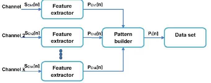
To develop and test the proposed approach for hand movement classification, the features 165
described above are first extracted from different channelsSCh1[n],. . . ,SChk[n]and placed in a dataset. 166
Each feature extractor (see Figure2) forms single or multiple features and its output is a vector 167
that represents a pattern of the formPChk[n] = [f eature1chk,f eature2chk,. . . ,f eatureNchk]. Next, the
168
derived features from the channels are transferred to the pattern builder that concatenates the instances 169
to generate an object containing the extracted features, and a label assigned for the class instances 170
Pi[n] = [PCh1[n],PCh2[n],. . . ,PChk[n],classlabel]. Figure2shows the dataset building block diagram. 171
Figure 2.Data set building block diagram.
2.5. Proposed classification methodology 172
2.5.1. Burg reflection coefficients 173
As mentioned in Section2.3, Burg autoregressive model introduces the forward and backward 174
prediction errors 175
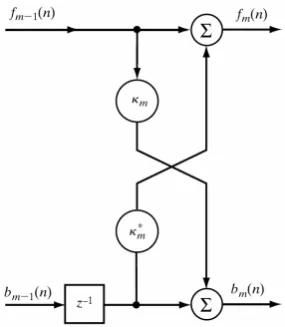
fm(n) =x(n) −xˆ(n),bm(n) =x(n−m) −xˆ(n−m) (18)
These errors are defined by the following recursive renovation equations of lattice linear prediction 176
Figure 3.Lattice filter prediction cascade diagram.
f0(n) =b0(n) =x(n),
fm(n) = fm−1(n) +Kmbm−1(n−1)m=1, 2, ...,p, bm(n) =K∗mfm−1(n) +bm−1(n−1)m=1, 2, ...p
(19)
The least squared error is 178
εm=
N−1
∑
n=m
[∣fm(n)∣2+ ∣bm(n)∣2] (20)
Minimizing expression20, the reflection coefficients are obtained [24]: 179
K∗ m=
− ∑N−n=m1+1fm−1(n)b ∗
m−1(n−1) 1
2∑nN−=m1+1[∣fm(n)∣t2+ ∣bm(n)∣2]
,m=1, 2, ...,p (21)
Reflection coefficients are the harmonic mean value of backward and forward error coefficient 180
cross correlation. The numerator is the cross correlation of the prediction errors and the denominator is 181
the smallest square estimation of these errors, so,∣Km∣ ≤1. The reflection coefficients (21) are computed 182
iteratively through the signal values; this is the reason they are proposed as features for classification 183
tasks as their complexity is linear, and there is no evidence of their usage in such tasks. 184
2.5.2. Classification model training 185
Classification models involved in this research work are Bayesian,Knearest neighbor, multilayer 186
perceptron, decision trees and support vector machines with different kernels. These classifiers are 187
available in machine learning tool WEKA [26] and were taken with the purpose of evaluating their 188
performance using different sEMG features. For the training phase, the following three datasets were 189
generated comprising 900 instances and 10 traits per channel: 190
● Time domain Data set (1)-(11): TD=[IEMG MAV SSI VAR RMS W L WAMP SSC ZC MYOP] 191
● Burg autoregressive coefficients (17): Arb=[Arb1Arb2. . . Arbn] 192
● Reflection coefficients: K=[K1K2. . . Kn] 193
The classification algorithms were trained once, and the performance was obtained by K-fold 194
cross validation withKvalue of 10 because they widely use it in state-of-the-art related works, and the 195
datasets lack of class unbalance. Moreover, each instance takes part in the training and testing set for 196
a single run of the learning algorithm. Burg autoregressive coefficients (17) were chosen instead of 197
a more accurate approximation [24]. After classifying three main datasets, K, Arb and TD features were 199
joined into a new dataset with patterns of the form ofX= [IEMG MAV SSI VAR RMS W L WAMP 200
SSC ZC MYOP Arb1Arb2. . . ArbnK1K2. . . Kn]; in order to evaluate how the interaction between 201
these different features is reflected in classification model performance. 202
2.5.3. Feature selection 203
Under the same validation method (k-fold cross validation), taking the dataset with instances in 204
the form of X, WEKA principal components (PC) and subset evaluation (SE) feature selection models 205
[26] applied to reduce the pattern dimensionality and select the less redundant and correlated attributes 206
for the classification task. Feature selection guarantees a reduction in dimensionality with or without a 207
degradation of the classifier model performance. As observed in Section2, some time domain features 208
rely on sEMG amplitude such as RMS and MAV, and others depend on counting a certain event 209
according to a threshold value. As a result, these attributes might contain a redundancy; also, the Burg 210
autoregressive coefficients and reflection coefficients are tied according to (17). Sequential forward 211
selection [27] strategy comprising taking just one of the different features used for dataset construction. 212
Another feature selection criterion is plus l – take away r algorithm - [27], based on takingl traits 213
from TD, K and Arb from X and remove the remaining r features, in such a way that the classification 214
performance remains high. If the exclusion of an attribute causes a lower than previous performance, 215
the removed sEMG characteristic is returned to the dataset because it is helpful for the class instance 216
assignation. This process is repeated until the dimensionality cannot be reduced without affecting the 217
classification rate. 218
3. Results 219
3.1. Datasets classification 220
Here, the results of the hand movement classification with separated datasets are presented. The 221
parameter changed in SVM model was kernel function. For the rest of models, the default Weka 222
parameters were not modified. Two values chosen forkin IBk arek=1 andk=numberof classes+1; 223
assigningk=6 would cause a tie between six classes; the extra value will establish the majority class. 224
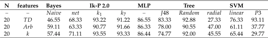
Table1describes the results obtained by classifying the hand movements with separated datasets. 225
Table 1.Classification results of TD, Arb and K datasets separately.
N features Bayes Ik-P 2.0 MLP Tree SVM
− − Naive net k1 k7 − J48 Random radial linear P3
20 TD 46.55 68.33 93.22 91.22 86.55 83.33 92.88 27.33 76.33 93.11 20 Arb 59.11 63.33 90.77 91.66 86.33 78.00 90.55 47.00 61.11 37.77 20 k 57.44 71.11 93.55 93.33 86.44 74.77 92.00 45.55 65.44 29.77
One can observe from Table1that TD dataset and the SVM with third order polynomial kernel 226
(P3 column) gives better decision borders than other kernels. The radial kernel yields the lowest 227
performance with Bayesian models; whereas the remaining models (trees and MLP) reached high 228
classification rates, IBk withk=1 obtained the highest. The dataset built only with maximal entropy 229
autoregressive coefficients (Arb column) is more appropriate to classify with the IBk considering 230
seven neighbours more than just one. Other learning algorithms such as MLP and decision trees 231
offer competitive classification rates (78% - 90.77%); Bayesian models overcome linear kernel support 232
vector machines with a performance of 63.33%. The best performance among the different datasets 233
is obtained using the reflection coefficient dataset K of the reflection coefficients, classifying 93.55% 234
of instances using IBkk=1. Despite Bayesian models and SVM still having a low performance, an 235
Table 2.Classification performance of combined datasets.
N features Bayes Ik-P 2.0 MLP Tree SVM
− − Naive net k1 k7 − J48 Random radial linear P3
40 k+TD 61.44 83.22 99.88 99.55 98.44 87.11 98.33 18.33 83.11 93.22 40 k+Arb 78.22 82.33 99.66 99.33 98.44 84.77 98.66 64.00 90.00 54.66 60 X 76.00 83.33 100.0 99.77 99.11 85.55 95.55 17.77 83.00 93.22
In Table2, by merging reflection coefficients and TD features for the training phase (K+TD), most 237
of the classifiers reach high performance, excluding naïve Bayes and radial kernel SVM. With a 0.22% 238
classification error, IBkk=1 got the best classification rate above the following models: IBkk= 7, 239
MLP, decision trees and 3thgrade polynomial kernel SVM. The resulting dataset of joining the Burg 240
maximal entropy reflection coefficients,K, and the Burg autoregressive coefficients, Arb, yield patterns 241
that are best classified by the IBk model with k value of one, slightly above the IBk usingk=7, MLP 242
and random forest. TheJ48 decision tree and Bayesian models offer high performances and are below 243
90% accuracy reached by linear kernel SVM; the other kernels have the lowest classification rates. 244
The combination of all features (TD, Arb, and K) results in a sixty-dimension feature vector, useful to 245
classify correctly all 900 dataset instances using the IBk withk=1; increasing the number of neighbors 246
tok=7 decreases the classification rate, but keeps on above the following competitive models, MLP 247
and random forest. Data distribution does not fit to a radial kernel, therefore, the SVM outputs the 248
lowest accuracy. 249
3.2. Feature selection classification performance 250
This subsection describes the results of dimensionality reduction trying to reach a higher 251
classification performance with as fewer traits as possible. After running the feature selection 252
algorithms, all instances kept on being classified correctly with 20 and 26 features with the nearest 253
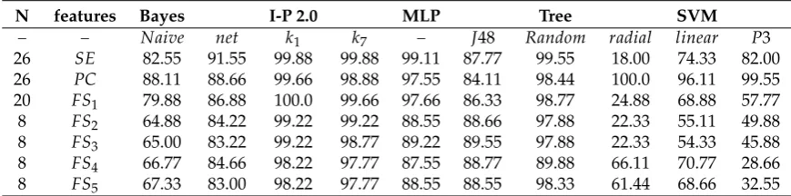
neighbours and support vector machine models, respectively (see Table3). SE traits exclude amplitude
Table 3. Classification performances using different feature vectors after feature selection: SE=[Ch1Arb(1,2,5,9,10), ch1k(1,2,3,4,9), Ch1WL, Ch1SSC, Ch1ZC, Ch1MYOP, Ch2Arb(1,2,4,5,10), Ch2k(1,5,7),Ch2WL,Ch2MYOP],FS1=[ARB(1,2,7,8,10), K(1,2,10),ZCC,MYOP],FS2=[Arb1, K1, ZCC, RMS],FS3=[Arb1,K1, ZCC, MAV],FS4=[Arb1,K1, MYOP, RMS]FS5=[Arb1,K1, MYOP, MAV].
N features Bayes I-P 2.0 MLP Tree SVM
− − Naive net k1 k7 − J48 Random radial linear P3
26 SE 82.55 91.55 99.88 99.88 99.11 87.77 99.55 18.00 74.33 82.00 26 PC 88.11 88.66 99.66 98.88 97.55 84.11 98.44 100.0 96.11 99.55 20 FS1 79.88 86.88 100.0 99.66 97.66 86.33 98.77 24.88 68.88 57.77 8 FS2 64.88 84.22 99.22 99.22 88.55 88.66 97.88 22.33 55.11 49.88 8 FS3 65.00 83.22 99.22 98.77 89.22 89.55 97.88 22.33 54.33 45.88 8 FS4 66.77 84.66 98.22 97.77 87.55 88.77 89.88 66.11 70.77 28.66 8 FS5 67.33 83.00 98.22 97.77 88.55 88.55 98.33 61.44 68.66 32.55 254
related values such as RMS, MAV and so on. They provide high classification rates with the exception 255
of the linear kernel SVM. The PC dataset was built with the combination of the less correlated features 256
resulting in a more uniform performance through all tested classifiers, reaching 100% performance 257
using the SVM with a radial kernel. TheFS1represents the result of the feature selection process; the 258
IBk with k=1 is still the highest and SVM with any kernel, the lowest. DatasetsFS2,FS3,FS4,FS5were 259
obtained taking the first reflection and autoregressive coefficients in combination with MYOP, ZCC, 260
RMS, MAV. These sets are of low pattern dimensionality and have high performance from 83% up 261
to 99.22% using the IBk withk=1(the highest), MLP, decision trees and Bayes net (the lowest); the 262
4. Discussion 264
The classification accuracy rate of different learning algorithms depends on the data distribution. 265
This behaviour is expected according to the “no-free-lunch theorems” [28], which state that the best 266
classification model for all datasets does not exist. The justification of why several models have to be 267
compared using the same dataset concurs with that statement. 268
While testing classifiers with separated datasets, Burg reflection coefficients K (21) are more 269
appropriate to be used in conjunction with the Bayes net and IBk models. Since K traits are needed to 270
compute the Burg autoregressive traits, Arb (17), their classification performances are similar. Besides, 271
TD features have different values which rely on amplitude or counting events. Therefore, the MLP, 272
decision trees, and linear and polynomial kernel SVM outputs have high accuracy. 273
Despite the Burg maximal entropy autoregressive and reflection coefficients being closely related, 274
the classification rate increases when these two traits take a part of the dataset. This means that they 275
are not redundant or irrelevant in feature construction tasks; however, as mentioned before, Arb 276
characteristics take more time to be computed because they rely on first computing the reflection 277
coefficients. In addition, as a result of combining three different theoretical frameworks attributes, the 278
highest classification rate is obtained. Hence, a synergy of different attributes is needed for a higher 279
accuracy in the sEMG classification tasks. 280
In Section3.2, opposite to the results in Table2, a high classification performance is reached 281
with 26 or fewer features. The fact that the feature vector X has at least 34 redundant or irrelevant 282
traits, which are necessary to be removed using feature selection tools can explain it. As a result, 283
different data distributions are obtained; for instance, principal component analysis performed by 284
WEKA produces a data distribution suitable for the support vector machine with a radial kernel since 285
all patterns are correctly classified. 286
Excluding the PC dataset, the best classifier for the remaining datasets is the IBk model with a 287
different number of neighbours used for class assignment, because the performance of the nearest 288
neighbors-based model depends onkvalue. For instance, TD and K dataset classification rate decreases 289
as a result of increasingkvalue, contrasting to what happens with Arb patterns (see Table1). This 290
behaviour is expected due to the classification phase applying the nearest neighbour to different classes 291
causing in the worst case a tie and a misclassified pattern. 292
The IBk advantage is its simple training phase that bases directly on the dataset compared to 293
Bayesian models that require the computation of probability distributions and cost function. The 294
design of the hidden layer of MLP can be complex and the time of back propagation error reducing 295
might be long. The decision trees as well as multilayer perceptron are hard to design, and they require 296
a pruning process to reduce irrelevant leaves and branches and the SVM hasO(n3)complexity to 297
establish support vectors. The kernel selection and design of the support vectors that best fits the data 298
distribution are needed. 299
An example of kernel selection can be seen from Table 1 with the TD dataset: using the polynomial 300
kernel, a high performance of 93.11% is reached, and merging the TD with K features an improvement 301
of 0.11% is achieved. This is a sign that most of the support vectors are found in the TD traits using 302
such a kernel. Another example is Arb and K traits: they are better classified with a linear kernel, and 303
by joining these two datasets, a considerable increase in the classification rate is obtained (see Table2) 304
as a consequence of more appropriate data for the support vector estimation. 305
The results that are considered for the discussion are those that was obtained using the same 306
signal dataset; otherwise, any comparison concerning the feature extraction and preprocessing stage 307
based on the classification performance would be unfair. 308
The feature extraction method presented in [22] yields fifty traits and reaches a high performance 309
(98.22%) with no previous signal treatment while the classification rates of 89.21% are obtained with the 310
empirical mode decomposition technique, which denoises the original signal in conjunction with sixty 311
four features proposed in [23]. Our methodology succeeded in classifying all 900 sEMG instances with 312
with just 8 traits producing the 99.22% correctly classified signals. Our preprocessing stage consists 314
only in the reduction of noisy samples and the subtraction of the myoelectric signal mean value, which 315
turns out to be effective due to it giving signals suitable to the framework of the developed feature 316
extraction tools, such as Burg reflection coefficients (21). 317
As shown in [23], decomposing sEMG causes an information loss that is reflected in the 318
classification rate; for this reason, all available signal information for the feature extraction task 319
were taken. 320
5. Conclusions 321
The results of hand movement classification of myoelectric signals using different traits have 322
been presented. The Burg linear autoregressive model yields to the reflection coefficients that have 323
been shown to be useful for the sEMG classification; these traits have shown a higher performance 324
that is increased with the standard time domain features and are less complex to compute than the 325
autoregressive coefficients. 326
A high classification rate has been reached using a simple preprocessing stage, which fits the 327
signals to the theory framework in the feature extraction tools. Low pattern dimensionality results from 328
removing redundant traits and building patterns with uncorrelated features such as Burg maximal 329
entropy reflection and autoregressive coefficients and considering different time domain features 330
related to the signal energy and to event counting. Despite a lower feature dimensionality, the 331
classification rate up to 100% has been achieved separately and with other kinds of uncorrelated 332
attributes for the hand movement identification. 333
The applications of the classification technique of signals presented in this work can lead to the 334
possible development of state-of-the-art active prosthetic devices, where the myoelectric classification 335
does not represent a challenge and the implementation of the classification algorithm can be performed 336
in an integrated low cost device. 337
338
Acknowledgments: 339
340
This work was partially supported by the Instituto Politécnico Nacional and CONACyT. 341
342
Conflicts of Interest: 343
344
The authors declare no conflict of interest. 345
References 346
1. De Luca, C.J. Electromyography. InEncyclopedia of Medical Devices and Instrumentation, Vols 1-4; John Wiley 347
& Sons, Inc., 2006. doi:10.1002/0471732877. 348
2. Raez, M.B.I.; Hussain, M.S.; Mohd-Yasin, F.; Reaz, M.; Hussain, M.S.; Mohd-Yasin, F. Techniques of EMG 349
signal analysis: detection, processing, classification and applications. Biological procedures online2006. 350
doi:10.1251/bpo115. 351
3. Lahmiri, S.; Boukadoum, M. Improved Electromyography Signal Modeling for Myopathy Detection. 352
2018 IEEE International Symposium on Circuits and Systems (ISCAS). IEEE, 2018, pp. 1–4. 353
doi:10.1109/ISCAS.2018.8350893. 354
4. Fuglsang-Frederiksen, A. The role of different EMG methods in evaluating myopathy, 2006. 355
doi:10.1016/j.clinph.2005.12.018. 356
5. Dostál, O.; Vysata, O.; Pazdera, L.; Procházka, A.; Kopal, J.; Kuchy ˇnka, J.; Vališ, M. Permutation entropy 357
and signal energy increase the accuracy of neuropathic change detection in needle EMG.Computational 358
6. Cler, M.J.; Stepp, C.E. Discrete Versus Continuous Mapping of Facial Electromyography for 360
Human-Machine Interface Control: Performance and Training Effects. IEEE Transactions on Neural Systems 361
and Rehabilitation Engineering2015. doi:10.1109/TNSRE.2015.2391054. 362
7. Brunelli, D.; Tadesse, A.M.; Vodermayer, B.; Nowak, M.; Castellini, C. Low-cost wearable multichannel 363
surface EMG acquisition for prosthetic hand control. 2015 6th International Workshop on Advances in 364
Sensors and Interfaces (IWASI). IEEE, 2015, pp. 94–99. doi:10.1109/IWASI.2015.7184964. 365
8. Copaci, D.; Serrano, D.; Moreno, L.; Blanco, D.; Copaci, D.; Serrano, D.; Moreno, L.; Blanco, D. A High-Level 366
Control Algorithm Based on sEMG Signalling for an Elbow Joint SMA Exoskeleton.Sensors2018,18, 2522. 367
doi:10.3390/s18082522. 368
9. Repnik, E.; Puh, U.; Goljar, N.; Munih, M.; Mihelj, M.; Repnik, E.; Puh, U.; Goljar, N.; Munih, M.; Mihelj, M. 369
Using Inertial Measurement Units and Electromyography to Quantify Movement during Action Research 370
Arm Test Execution. Sensors2018,18, 2767. doi:10.3390/s18092767. 371
10. Merletti, R.; Farina, D. Surface Electromyography: Physiology, Engineering and Applications; John Wiley & 372
Sons, 2016. doi:10.1002/9781119082934. 373
11. Hsueh, Y.H.; Yin, C.; Chen, Y.H. Hardware System for Real-Time EMG Signal Acquisition and 374
Separation Processing during Electrical Stimulation. Journal of Medical Systems 2015, 39, 88. 375
doi:10.1007/s10916-015-0267-6. 376
12. Resnik, L.; Huang, H.; Winslow, A.; Crouch, D.L.; Zhang, F.; Wolk, N. Evaluation of EMG pattern 377
recognition for upper limb prosthesis control: a case study in comparison with direct myoelectric control. 378
Journal of NeuroEngineering and Rehabilitation2018,15, 23. doi:10.1186/s12984-018-0361-3. 379
13. Venugopal, G.; Navaneethakrishna, M.; Ramakrishnan, S. Extraction and analysis of multiple time window 380
features associated with muscle fatigue conditions using sEMG signals. Expert Systems with Applications 381
2014. doi:10.1016/j.eswa.2013.11.009. 382
14. Nazmi, N.; Abdul Rahman, M.; Yamamoto, S.I.; Ahmad, S.; Zamzuri, H.; Mazlan, S. A Review of 383
Classification Techniques of EMG Signals during Isotonic and Isometric Contractions. Sensors2016, 384
16, 1304. doi:10.3390/s16081304. 385
15. Chowdhury, R.H.; Reaz, M.B.I.; Ali, M.A.B.M.; Bakar, A.A.A.; Chellappan, K.; Chang, T.G. Surface 386
electromyography signal processing and classification techniques. Sensors (Basel, Switzerland)2013. 387
doi:10.3390/s130912431. 388
16. Bozkurt, M.R.; Suba¸si, A.; Köklükaya, E.; Yilmaz, M. Comparison of AR parametric methods with 389
subspace-based methods for EMG signal classification using stand-alone and merged neural network 390
models. Turkish Journal of Electrical Engineering and Computer Sciences2016. doi:10.3906/elk-1309-1. 391
17. Phinyomark, A.; Limsakul, C.; Phukpattaranont, P. Application of wavelet analysis in EMG feature 392
extraction for pattern classification. Measurement Science Review2011. doi:10.2478/v10048-011-0009-y. 393
18. Veer, K.; Sharma, T. A novel feature extraction for robust EMG pattern recognition. Journal of Medical 394
Engineering & Technology2016,40, 149–154. doi:10.3109/03091902.2016.1153739. 395
19. Liu, Y.H.; Huang, H.P.; Weng, C.H. Recognition of Electromyographic Signals Using Cascaded Kernel 396
Learning Machine. IEEE/ASME Transactions on Mechatronics2007. doi:10.1109/TMECH.2007.897253. 397
20. Al-Angari, H.M.; Kanitz, G.; Tarantino, S.; Cipriani, C. Distance and mutual information methods for EMG 398
feature and channel subset selection for classification of hand movements.Biomedical Signal Processing and 399
Control2016. doi:10.1016/j.bspc.2016.01.011. 400
21. Khezri, M.; Jahed, M. A Neuro–Fuzzy Inference System for sEMG-Based Identification of Hand Motion 401
Commands. IEEE Transactions on Industrial Electronics2011,58, 1952–1960. doi:10.1109/TIE.2010.2053334. 402
22. Ruangpaisarn, Y.; Jaiyen, S. SEMG signal classification using SMO algorithm and singular value 403
decomposition. Proceedings - 2015 7th International Conference on Information Technology and Electrical 404
Engineering: Envisioning the Trend of Computer, Information and Engineering, ICITEE 2015, 2015. 405
doi:10.1109/ICITEED.2015.7408910. 406
23. Sapsanis, C.; Georgoulas, G.; Tzes, A.; Lymberopoulos, D. Improving EMG based classification of basic 407
hand movements using EMD. Proceedings of the Annual International Conference of the IEEE Engineering 408
in Medicine and Biology Society, EMBS, 2013. doi:10.1109/EMBC.2013.6610858. 409
24. Haykin, S.S.Adaptive filter theory; Pearson, 2014. doi:0130901261. 410
25. Burg, J.P. Maximum entropy spectral analysis. PhD thesis, Stanford, 1975. doi:doi.wiley.com/ 10.1002/ 411
26. Witten, I.H.; Frank, E.; Trigg, L.; Hall, M.; Holmes, G.; Cunningham, S.J. Weka : Practical Machine Learning 413
Tools and Techniques with Java Implementations. Proceedings of the ICONIP/ANZIIS/ANNES’99 414
Workshop on Emerging Knowledge Engineering and Connectionist-Based Information Systems, 1999, pp. 415
192–196. doi:10.1.1.16.949. 416
27. Ciaccio, E.J.; Dunn, S.M.; Akay, M. Biosignal Pattern Recognition and Interpretation Systems. IEEE 417
Engineering in Medicine and Biology Magazine1994. doi:10.1109/51.265792. 418
28. Wolpert, D.H.; Macready, W.G. No free lunch theorems for optimization. IEEE Transactions on Evolutionary 419
Computation1997. doi:10.1109/4235.585893. 420