GAMBLE, JENNIFER PAMELA. Complex and Dynamic Network Analysis: A Topological Perspective. (Under the direction of Dr. Hamid Krim.)
This dissertation develops and applies topological methods for the analysis of complex and dynamic networks. In contrast to the term ‘topology’ used in traditional network analysis, here we use the term in the sense of algebraic topology. The field of topological data analysis (TDA) has blossomed in recent years, allowing researchers to analyze point cloud data sets using methods that take into account the ‘shape’ of the data. This includes geometrical features, as well as topological features such as connected components, loops, and voids. These methods have been applied with great success to data sets which are naturally embedded in a metric space (such as Euclidean space), because distances between points can be used to form a parameterized sequence of spaces, and studying the changing topology of this sequence gives information about both the topology and geometry of the data under analysis.
In our setting, the input data are simply graphs, consisting of vertices connected by (undirected, unweighted) edges, with no underlying metric other than the graph distance between vertices. We demonstrate how one can still consider the ‘shape’ of such objects in a topologically-informed way, using a simplicial complex representation, and that such a viewpoint has great advantages.
We first apply this methodology to analyzing coverage properties in dynamic sensor networks. The dynamic sensor network under consideration is studied through a series of snapshots, and is represented by a sequence of simplicial complexes, built from the communication graph of the network at each time point. A method from TDA called zigzag persistent homology takes this se-quence of simplicial complexes as input, and returns a ‘barcode’ containing the birth and death times of topological features in this sequence. We derive useful statistics from this output for ana-lyzing time-varying coverage properties.
quantitative descriptor of the dynamic network coverage.
by
Jennifer Pamela Gamble
A dissertation submitted to the Graduate Faculty of North Carolina State University
in partial fulfillment of the requirements for the Degree of
Doctor of Philosophy
Electrical Engineering
Raleigh, North Carolina
2015
APPROVED BY:
Huaiyu Dai Patricia Hersh
Brian Hughes Hamid Krim
I first have to acknowledge my advisor, Dr. Hamid Krim, without whom this would not have been possible. I especially valued the format of his weekly group meetings, which required us to express our ideas clearly and regularly, and greatly increased our breadth of knowledge by keeping on top of the research of our labmates. I know of very few university professors who devote this many hours per week to meeting with their students. Additionally, his bi-weekly seminar series brought count-less world-class researchers to the department, and having the opportunity to meet with them not only yielded many helpful insights, but required us to become comfortable presenting our work to professional audiences. I would also like to thank the rest of my advisory committee: Dr. Huaiyu Dai, Dr. Brian Hughes, and Dr. Patricia Hersh, as well as Dr. Yannis Vinotis for substituting for Dr. Hughes during my final defense. I greatly value your time and advice, and your comments and suggestions along the way have always been helpful and insightful.
The person who has had the greatest impact on my research life is my onetime labmate, fre-quent co-author, and dear friend, Harish Chintakunta. He has the true inquiring spirit all academics should aspire towards, and in many ways he is the one who taught me, both directly and indirectly, how to do research. I often question whether I would have even completed my PhD, had it not been for Harish.
The daily life of a graduate student is in the lab, and as such, I have been very happy to share it with Scott Clause, Tian Wang, Xiao Bian, Adam Wilkerson, Saba Emrani, Deokwoo Lee, Sheng Yi, Shahin Mahdizadehaghdam, Hui Guan, Sally Ghanem, and Erik Skau. Over the years we developed many tight bonds, and I really value both their camaraderie and amazing intellectual resources. I was also pleased to work with and learn from our postdocs, Athanasios Gentemis, and Han Wang, who are both great people as well.
My parents Ken and Donna, are the personification of unconditional love. The fact that my two sisters and I are all profoundly happy, doing completely different things, on opposite sides of the world, speaks to our parents love and guidance in encouraging us to follow our own paths. Katie and Meggie, I love you too! Thank goodness for Skype. I’d also like to thank Tia Halliday (my bff ), and my wonderful in-laws Barb and Gabby for all their love and support.
My sweet Lucy, who made me a mother. You have added so much joy to my life, with a power I couldn’t have anticipated.
LIST OF TABLES . . . .viii
LIST OF FIGURES. . . ix
Chapter 1 Introduction. . . 1
Chapter 2 Coordinate-Free Quantification of Coverage in Dynamic Sensor Networks . . . 5
2.1 Introduction . . . 5
2.2 Preliminaries . . . 9
2.2.1 Simplicial homology . . . 10
2.2.2 Simplicial complex representation of a sensor network . . . 14
2.3 Coverage properties of dynamic networks . . . 18
2.3.1 Zigzag persistent homology . . . 18
2.3.2 Barcodes as descriptors of coverage . . . 19
2.3.3 Comparing mobility models . . . 24
2.4 Coordinate-free estimation of hole size . . . 32
2.5 Tracking representative cycles . . . 37
2.5.1 Examples . . . 38
2.6 Conclusions and Future Work . . . 43
Chapter 3 Adaptive Tracking of Representative Cycles in Zigzag Persistent Homology. . . 44
3.1 Introduction . . . 44
3.2 Terminology and notation . . . 45
3.2.1 Simplicial complexes and homology . . . 45
3.2.2 Zigzag persistence . . . 46
3.2.3 Right filtration . . . 48
3.3 Tracking representative cycles . . . 51
3.3.1 Motivation . . . 51
3.3.2 Algorithm . . . 55
3.4 Correctness . . . 60
3.5 Conclusion . . . 69
Chapter 4 Node dominance: revealing core-periphery structure in social networks. . . 70
4.1 Introduction . . . 70
4.2 Background . . . 75
4.2.1 Simplicial homology . . . 75
4.2.2 Node dominance . . . 77
4.3 Properties of core and periphery . . . 82
4.3.1 Network flow . . . 83
4.3.2 Community structure . . . 85
4.3.3 Global structure . . . 87
4.4.3 Community detection . . . 95
4.5 Conclusion . . . 101
Chapter 5 Conclusions and Future Work. . . .104
5.1 Conclusions . . . 104
5.2 Future Work . . . 105
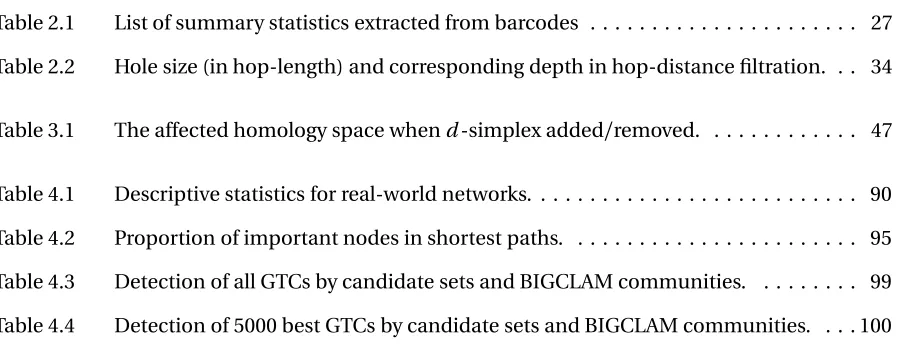
Table 2.1 List of summary statistics extracted from barcodes . . . 27
Table 2.2 Hole size (in hop-length) and corresponding depth in hop-distance filtration. . . 34
Table 3.1 The affected homology space whend-simplex added/removed. . . 47
Table 4.1 Descriptive statistics for real-world networks. . . 90
Table 4.2 Proportion of important nodes in shortest paths. . . 95
Table 4.3 Detection of all GTCs by candidate sets and BIGCLAM communities. . . 99
Figure 2.1 Simplices and a small simplicial complex . . . 13
Figure 2.2 Topological space with first homology of dimension two. . . 13
Figure 2.3 Coverage region and Rips complex for a sensor network. . . 16
Figure 2.4 Illustration of ‘missed’ coverage hole. . . 17
Figure 2.5 Barcode and persistence diagram. . . 20
Figure 2.6 Sequence of Rips complexes and their union complexes. . . 22
Figure 2.7 Discrete Brownian and Straight Line mobility patterns. . . 26
Figure 2.8 Barcodes for realizations of Discrete Brownian and Straight Line. . . 28
Figure 2.9 Histograms comparing number of bars in two mobility patterns. . . 30
Figure 2.10 Comparison of counts of lifetime lengths for the two patterns. . . 31
Figure 2.11 Mean interval coverage for the two patterns. . . 31
Figure 2.12 Proportion of area covered over time for the two patterns. . . 32
Figure 2.13 Illustration of hop distance filtration. . . 34
Figure 2.14 Coverage hole area vs homological features. . . 36
Figure 2.15 Tracking representative cycles in a dense network. . . 39
Figure 2.16 Network with an expanding failure region. . . 41
Figure 2.17 Weighted barcode for expanding failure region. . . 42
Figure 2.18 Tracking perimeter formed by mobile guards. . . 42
Figure 3.1 The coverage region and communication graph for a sensor network. . . 52
Figure 3.2 The Rips complex and Rips shadow of the communication graph. . . 53
Figure 3.3 The four first homology changes, and corresponding representative cycles. . . . 56
Figure 4.1 Nodev dominated by nodew. . . 80
Figure 4.2 Log betweenness centrality vs degree (DBLP-top, Amazon-bottom). . . 92
1
INTRODUCTION
The fundamental viewpoint motivating this work is that incorporating topological features when analyzing complex data can yield surprising and informative results about the data’s structure, which are not obtainable from other methods. In the case of network analysis, the use of higher-order information, such asn-tuple relationships between nodes, is encoded using simplicial com-plexes. This allows for topological information to be considered, which opens access to a wealth of mathematical tools.
of the time-varying coverage of a network in a completely coordinate-free manner, using only the adjacency matrix for the communication graph at each time point. In the second case, the local property of node dominance yields a distributed algorithm for computing a core-periphery de-composition of a social network, where the core is shown to be essential for the network in terms of network flow and global structure, and additionally the peripheral components give information about the community structure that yields an effective algorithm for community detection.
“Topological data analysis” (TDA), is a somewhat broad term which can be meant to describe any data analysis methods which use a topological space (or sequence of spaces) built from the data, and use features of this space (topological, geometric, or other) to describe the data set. This is often interpreted as studying the ‘shape’ of the data, because topological features include things like the number of connected components, loops, or voids in a space, and because the topological space is usually constructed using a function on the metric space the data lie in (incorporating ge-ometric information). As a field of study, TDA was not born until nearly the turn of the 21st century. Prior to that, algebraic topology was viewed as a pure form of mathematics, or ’math for math’s sake’, without express purpose for reworld applications. Since it is a field of mathematics which uses al-gebraic objects to study topological spaces, alal-gebraic topology is very broad and can become quite abstract. Later on, when we discuss the special case of simplicial homology theory in Section 2.2.1, we see that it will become quite concrete (reducing to linear algebra computations), and extremely useful for our applications.
The advent of the persistent homology algorithm[16] [45]and its mathematical formalization [62]are often considered the turning point, which allowed topological features to be considered
applicable to the study of data sets (although some earlier methods in computational geometry [17]and size theory[19]had a topological flavor as well). Many of the relevant notions had been
com-plex required a choice of parameter value, and that the resulting topological features are extremely non-robust to perturbations in the underlying data set. The key to persistent homology, was that it took a multi-resolution approach by considering asequence of simplicial complexes, over a range of parameter values. Studying the changing homology of the sequence gave information about the topologyand geometry of the data set, and the summary for this changing sequence of spaces (cru-cially) also had good stability properties[12] [11]. A second algorithm which has become synony-mous with TDA is the mapper algorithm[49], which also builds a simplicial complex to represent a dataset, but in this case the complex obtained is dependent on the choice of a function, so one may study a single data set through different “lenses” by using different choices of functions. For some excellent survey articles of persistent homology and topological data analysis, see Ghrist[23]and Carlsson[6]. Currently, the theory and applications of TDA are predominantly oriented towards the persistent homology and mapper algorithms and their generalizations. It is important to note that these methods are motivated by applications in data analysis, where the data lie in a metric space (oftenn), and it is natural to use parameter and function values relative to this metric.
In this dissertation, the data structures we consider are fundamentally different from the point cloud data in typical TDA applications. We consider network (or graph) structures, which consist only of vertices, and edges connecting them. They are combinatorial in nature, and for our applica-tions the edges are unweighted, undirected, and connect two distinct vertices, so the only notion of distance between two vertices is the graph distance between them. We propose and explore ap-plications of methods for network analysis which are topologically-motivated, and we see that, as in the case with traditional TDA methods on point cloud data, the incorporation of topological fea-tures and ideas into the existing network analysis toolbox yields greater insights into the structure of our data, with fewer assumptions for the input (in the sensor network case) and more computa-tional efficiency (in the social network setting).
dis-tances (edge lengths) are known. Only binary information about which nodes are within commu-nication range at each time point is available, and through a combination of methods from com-putational topology, along with a novel algorithm, we are able to obtain a quantitative descriptor of the dynamic network coverage, which includes the number of holes at each time point, as well as estimated hole size and duration.
The algorithm is described in detail in Chapter 3. It takes the sequence of simplicial complexes, and chooses specific representative cycles for the homology classes at each time point, which are geometrically-relevant.
Finally, in Chapter 4 we turn our attention to study large-scale social networks. Here, we use topology-preserving collapses[4] [54]of the network to identify nodes which belong to a ‘core’, and develop theoretical results involving the properties of this core and the remaining periphery. The nodes in the core are seen to be very important to the global structure of the network, as well as network flow. Moreover, the peripheral components are related to the community structure of the network, and we propose an algorithm for their use in community detection, which is seen to per-form well against a state-of-the-art method for overlapping community detection in large networks. Results are placed in the context of existing theories of social network structure, and support the view that overlapping communities yield a core-periphery network structure.
2
COORDINATE-FREE QUANTIFICATION
OF COVERAGE IN DYNAMIC SENSOR
NETWORKS
The paper this chapter is based on was published inSignal Processing. See[22]or arXiv:1411.7337.
2.1
Introduction
over a region, with each sensor (or ‘node’) gathering data about its local environment for purposes of monitoring, detecting or reporting. In recent years, the study of wireless sensor networks has sig-nificantly increased, with research into methodologies for the different layers of the sensor network protocol stack (physical, data link, network, transport and application layers), each developing into their own sub-field. Areas of application include military, industrial, and environmental monitor-ing and trackmonitor-ing. See[3]and[60]for surveys of the field.
A particular problem in sensor networks which quickly gained research interest is the so-called ‘coverage problem’[28]. Given a set of (typically homogeneous) sensors, each with the ability to sense some region of immediate proximity to it, one wishes to make statements about the sensing ability of the entire network, taken as a whole. An initial question is whether every point in a region of interest is covered by at least one sensor. As sensor networks developed, it was no longer realistic to assume a static network, and node mobility became a factor in network analysis and design. It became clear that mobility of nodes could be considered for initial deployment[44] [27], as well as for improving coverage over time[36]; thus, the development of methods to study dynamic, or time-varying sensor networks has become increasingly important.
The availability of geometric information, such as global coordinates for the nodes, or distances between them, is often an overassumption. Instead, ‘coordinate-free’ methods compute network properties using only local, binary information about which nodes are within communication range of each other. De Silva and Ghrist[47]were the first to propose a rigorous method for determining coverage which did not require location or distance information, by invoking tools from simplicial homology theory (see Section 2.2 for details). Such homological methods are able to give guaran-tees that a network is covered at a single time point, or over a time interval, using only coordinate-free data.
Other researchers have used coordinate-free data to study network coverage by detecting ap-proximate boundaries of coverage holes in static networks. Some methods (such as in[30]or[35]) define interior nodes using specifically structured sub-graphs (‘flowers’ or ‘3MeSH rings’, respec-tively), while another method defines boundary nodes by using breaks in iso-contours formed by hop distance from a base node[20]. One method estimates the boundary by using a multi-step procedure built using the cuts in a shortest path tree which ‘forks’ around coverage holes[51]. All of these methods can obtain good experimental results, but are relatively dependent on the net-work having a high density, so the holes are large compared to the distances between neighboring sensors[29].
spe-cific cycles in the network characterizing the coverage holes over time, which aid in estimating the size of the holes.
The method we describe here is the only one currently available which can quantify the age dynamics in a coordinate-free network. We will also see that it correlates well with other cover-age measures which utilize full geometric information. Further, the barcode includes information about how coverage holes form, merge, split and close in the time-varying network, which is not available using existing methods (whether geometric information is included or not). In the past, homological methods have been able to give guarantees that a network is covered at a single time point, or over a time interval, while geometric methods have been used to obtain summary statis-tics which describe the time-varying nature of the network coverage. Here, we use homological, coordinate-free methods to obtain a descriptor of the dynamic network coverage.
As our primary contributions, we propose how the ‘barcode’ output from zigzag persistence can be used as a quantitative descriptor of time-varying coverage in a network, and moreover describe an algorithm we developed for choosing a specific geometrically-relevant cycle for each coverage hole in the network at each time point. The utility of the barcode is illustrated by using it to quantify and compare coverage dynamics for different models of sensor mobility. Our novel representative cycles are used in conjunction with a hop distance-based method to obtain size estimates for the holes, and this information is incorporated back into the barcodes, giving a visual and quantitative summary of the dynamic network coverage. Further examples demonstrate the effectiveness of this descriptor in tracking small coverage holes appearing in dense networks, in identifying expanding failure regions, and in monitoring the maintenance of a protective barrier of mobile sensors around a guarded region.
it allows. Section 2.4 details the hop distance-based filtration, and its use in estimating hole sizes for a given simplicial complex. Section 2.5 provides an outline of our method for obtaining specific representative cycles (which will be described in full detail in Chapter 3), and how these cycles can be used with the hop distance filtration to enhance the barcode with estimated size information for each bar at each time point. This is followed by examples illustrating the utility of the method, and by concluding remarks.
2.2
Preliminaries
The adopted sensor network coverage model assumes homogeneous, isotropic sensors with sens-ing radiusr, so that each sensor is at the center of its associated coverage region, which is a disk of radiusr. This ‘Boolean disk coverage model’ is the most widely used sensor coverage model in the literature[50]. Throughout this chapter, we will assume that the network consists ofnsensors, indexed 1 throughn. If sensoriis located atxi∈2, then denote the disk of radiusr centered atxi
asB(xi,r). Then the coverage region, for the entire network, is the union of all such disks:
=
n
i=1
B(xi,r). (2.1)
the entire network[47], using reasonably coarse local information. The local information required at each sensor is simply a list of the other nodes within a known communication range.
2.2.1 Simplicial homology
The theory of homology has a long and rich history, with results available in much greater gener-ality than necessary for our purposes here (see[25]for a good introduction to algebraic topology, including homology theory). The situation we will be considering is when the spaces under analy-sis are simplicial complexes, yielding matrix calculations for computing homology. First, we define a simplicial complex, and its homology.
Definition: Ak -simplexis a set of k+1 vertices, or singleton elements. Any subset of thek+1
vertices forming a simplex is called afaceof the simplex, where each face is, itself, also a simplex. Asimplicial complex,K, is a set of simplices such that any simplex inK also has all of its faces inK.
Definition: (Homology)Given a simplicial complex K we build thechain spaces C0,C1, C2, . . .,
whereCk is the vector space formed by using thek-simplices as basis elements. We then encode
information about the specific structure of the simplicial complex in theboundary maps∂1,∂2, . . .,
where
∂k:Ck→Ck−1
describes explicitly how thek-simplices are connected to the(k−1)-simplices. Fork-simplexσ= [v0,v1, . . .,vk], the boundary map∂k mapsσonto the alternating sum of its faces:
∂kσ=
k
i=0
(−1)i[v0, . . ., ˆvi, . . .,vk]
where ˆvi indicates the vertexvi removal. Note that the above definition of the boundary operator
depends on the initial ordering of the simplex, which is referred to asorientation. The simplices are assigned arbitrary orientations. Then thekt hhomology groupis defined to be
Hk(K) =ker(∂k)/im(∂k+1)
and thekt hBetti number(denotedβ
k) of the simplicial complexK is the rank ofHk(K).
To understand this definition, let us look at what ker(∂k)and im(∂k+1)mean individually. In
general,∂k maps ak-simplexσonto its boundary (which is made up of(k −1)-simplices), so if
σ= [vi,vj]is an edge, then∂1σ=vj−vi is the difference ofσ’s vertices. Similarly, ifσ= [vi,vj,vk]
is a triangle (a 2-simplex), then∂2σ= [vj,vk]−[vi,vk] + [vi,vj]is the alternating sum of its edges.
An elementc in the chain spaceCk is just a linear combination ofk-simplicesσ1, . . .,σnk,
c =
nk
i=1
and can be written as a vectorc = [a1, . . .,ank]of lengthnk=(# ofk-simplices inK). The coefficients
aicome from a field(such as the real numbers), but we choose to perform our computations over
the field2={0, 1}(in this case, the interpretation is that simplices with nonzero coefficients are
the ones present in the chainc). The boundary operator∂k is written as ank−1×nk matrix, so the computation of the boundary for any chain reduces to the matrix multiplication∂kc. Any chain
with boundary zero (i.e. anyc such that∂kc =0) is called acycle, and so ker∂k is the set of allk
-cycles. In particular, the boundary of a simplex will form a cycle, which implies that all boundaries are themselves cycles (i.e. im∂k+1⊆ker∂k). This also implies the general property that∂k∂k+1=0.
We can now reinterpret the definition of homology as “cycles which are not boundaries”.
Definition: Two cyclesc1andc2arehomologous(writtenc1∼c2) if their difference can be written
as a linear combination of boundaries. The set of all cycles that are homologous to a given cycle (sayc) is called ahomology class(denoted[c]). All cycles in the same homology class will surround exactly the same hole (or set of holes). When a specific cycle is chosen to represent an entire homol-ogy class, it is called arepresentative cycle. The span of the homology classes defined byk-cycles form thekt hhomology space.
It is in this sense that the rank of the kt h homology group (the Betti numberβk) counts the
number ofk-dimensional ‘holes’ in the simplicial complex. Intuitively,β0counts the number of
connected components, β1 counts the number of ‘holes’ as we normally think of them (empty
regions that one can form a loop around),β2counts the number of enclosed voids, and higher-dimensional homology is defined analogously.
In Figure 2.1, the cycle formed by edges[v2,v3],[v3,v4], and[v2,v4]is the boundary of the triangle
[v2,v3,v4], and thus is equivalent to zero (trivial) with respect to homology. The cycle formed by
edges[v1,v2],[v2,v4],[v4,v5], and[v1,v5], which we denote byc, cannot be written as the boundary
Figure 2.1Simplices and a small simplicial complex
c∼0 c1
c2 c1+c2
A final concept to highlight is that of ahomology basis. As seen in the above definitions, given a simplicial complexK, thekt h homology groupHk(K)is a vector space of dimensionβk, and
therefore any linearly independent set ofβk homology classes form a basis for Hk(K). As an
ex-ample, consider Figure 2.2, which illustrates a space with two holes (soβ1=2). The cyclec does not surround any holes, and is homologous to zero (i.e. it is trivial). The homology class[c1]
con-tains all cycles which surround only the righthand hole, and is represented by cyclec1. Similarly,c2
represents the homology class of cycles surrounding the lefthand hole. Note that the cyclec1+c2
is homologous to the sum of the cyclesc1andc2. Thus, this space has three distinct, non-trivial
homology classes:[c1],[c2], and[c1+c2], any two of which form a basis for the first homology (eg.
{[c1],[c2]}form a basis, as does{[c1],[c1+c2]}). Given a compact region of the plane, such as the
one shown, there exists acanonical basisfor its first homology, namely the basis with one homol-ogy class surrounding each of the holes ([c1]and[c2]in our example). This result is a specific case of the more general principle of Alexander Duality (see, for example Ch. 5 of[39]). The concept of a canonical homology basis will become relevant for us again in Section 2.5, where we describe our method for choosing a set of representative cycles in an attempt to approximate the canonical basis for the coverage area of a sensor network.
2.2.2 Simplicial complex representation of a sensor network
For the purposes of analyzing the coverage region of a sensor network, we are interested in comput-ing the homology of(the coverage region for the network - defined in Equation (2.1)). Specifically, we are interested inβ1=rank(H1()), the rank of the first homology group, to determine how many
and the disk of radiusr centered atxiis denotedB(xi,r).
Definition: ACech complexˇ contains thek-simplex formed by vertices
{v0,v1, . . .,vk}whenever
k
i=0
B(xi,r)=.
Definition: AVietoris-Rips complex(also referred to as a Rips complex) includes thek-simplex
formed by vertices{v0,v1, . . .,vk}whenever
B(xi,r)∩B(xj,r)=for all 0≤i<j≤k.
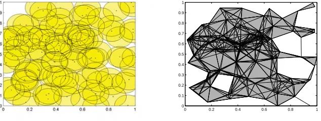
In other words, the ˇCech complex contains the higher-dimensional simplex formed by a group of sensors whenever all the coverage disks of those sensors have a nonempty intersection, and the Rips complex contains the higher-dimensional simplex whenever the coverage disks of a group of sensors all intersect pairwise. The coverage region formed by the union of coverage disks for a sensor network is shown in Figure 2.3 (left), with the associated Rips complex (right). Note that com-putation of the(k+1)-wise intersection of disks in the ˇCech definition requires precise geometric information about the relative locationsxiof the sensors. For the Rips complex, on the other hand,
ˇ
Cech complex reflects the true homology of the coverage region).
0 0.2 0.4 0.6 0.8 1
0 0.1 0.2 0.3 0.4 0.5 0.6 0.7 0.8 0.9 1
Figure 2.3Coverage region and Rips complex for a sensor network.
The configuration displayed in Figure 2.4 also illustrates one of the properties of the ˇCech com-plex: it has the exact same homology (number of holes) as the coverage region, while the Rips complex can ‘miss’ such small coverage holes. The worst-case detection of missed area is when the three nodes form an equilateral triangle with edge lengths 2r, is witnessed network-wide when the sensors lie on a hexagonal lattice. In this case the holes account for∼7% of the total area, and are not detected by the Rips complex. In practice, when the nodes are distributed uniformly and randomly, we found the holes missed by the Rips complex amount to1% of the total area (sim-ulations over a range of network sizes and node densities showed instances where the area of the ‘missed’ holes was up to 0.15% of the total area, but more typically they accounted for less than 0.03% of the total area).
com-Figure 2.4Illustration of ‘missed’ coverage hole.
munication to infer whether global coverage is achieved. They additionally consider a problem in dynamic networks: does anevasion path exist and allow an intruder to remain undetected over a time interval?. Their results give conditions which will guarantee that no such evasion path exists. For our purposes, we will understand that although the holes detected by the first homology of the Rips complex do differ from the holes in the coverage region (in exactly the way described above), the holes which are missed are extremely small relative to the size of the network. We will therefore use the homology computed using the Rips complex as a sufficient approximation. This is a particularly safe assumption in the time-varying case, because a very small hole which remains very small over time is justifiably ignored. Throughout, when we discuss ‘network coverage’, we are referring to the coverage as characterized by the Rips complex.
We now consider a time-varying network, which again has only pairwise communication infor-mation at each time point. We next present a method which, in addition to detecting global cov-erage, will track homological features over time, and provide information about the number and duration of coverage holes.
2.3
Coverage properties of dynamic networks
2.3.1 Zigzag persistent homology
Zigzag persistent homology is a recently developed computational method to track homological features (such as those described in Section 2.2) through a sequence of spaces. In our problem setting, where sensor networks are represented by simplicial complexes, and the first homology detects coverage holes, we employ this method to tell us about coverage holes in a time-varying sensor network. While we give a brief summary here, we defer to[8]and[7]for complete mathe-matical and algorithmic details (respectively) of zigzag persistence.
We use zigzag persistent homology to study a sequence of simplicial complexes
K1↔K2↔. . .↔Kn.
Call this sequence, and assume each map ‘↔’ is an inclusion: either ‘forward’ asKi→Ki+1
or ‘backward’ asKi←Ki+1. This sequence is studied by computing the associated homology spaces
to obtain thezigzag persistence module
Hp() =Hp(K1)↔Hp(K2)↔. . .↔Hp(Kn) (2.2)
One of the main theorems in the theory of zigzag persistent homology, is that such a module can be uniquely decomposed. EachHp(Ki)is a vector space, and the module in Equation (2.2) can
for some range[b,d], where 1≤b≤d ≤n, and zeros outside of this range (see[8]for details). The intervals in this decomposition are interpreted as the lifetimes of individual homological features in the sequence, which are summarized by their birth and death times (bandd). In the sensor net-work setting, the decomposition of the zigzag persistence module for the first homology gives a list of birth and death times of the one-dimensional homological features in the sequence. These ho-mological features describe the time-varying coverage of the network, in a way described precisely in Section 2.3.2. The multi-set of birth and death times
Pers() ={[bj,dj],}
is the zigzag persistence of our sequence of spaces, and is represented pictorially in two common ways. The first is a barcodewhere the x-axis represents timet, the y-axis represents individual homological features, and each feature is depicted as a horizontal line from its birth time (bi) to
death time (di). The second visual representation is apersistence diagram, which plots the points
(bi,di)on two-dimensional coordinate axes. Thus, all points lie above the diagonal (death occurs after birth), and points further from the diagonal indicate longer lifetimes. Figure 2.5 shows the barcode (left) and persistence diagram (right) corresponding to Pers() ={[2, 9],[4, 7],[6, 8],[9, 10]}, as an example.
This output of a discrete set of birth and death times for homological features can be used to quantify the time-varying coverage for a given dynamic sensor network, as described in the follow-ing section.
2.3.2 Barcodes as descriptors of coverage
0 1 2 3 4 5 6 7 8 9 10 0 0.5 1 1.5 2 2.5 3 3.5 4 4.5 5 Barcode Time Feature
0 1 2 3 4 5 6 7 8 9 10 11
0 1 2 3 4 5 6 7 8 9 10 11 Birth time Death time Persistence diagram
Figure 2.5Barcode and persistence diagram.
the first homology of this complex is used to determine coverage of the network. We now consider a time-varying sensor network, whose communication graph (and thus its associated simplicial complex) is available at a sequence of discrete time points. It is assumed that each sensor has a unique node identification number in{1, . . .,n}, and so a correspondence can be made between the simplicial complex at one time point and the next.
Given simplicial complexes at two consecutive time pointsti andti+1, we do not have a direct
inclusion mapKti → Kti+1 orKti ← Kti+1, because there may be a number of simplices that are
present inKtibut not inKti+1, and vice versa. To employ the machinery of zigzag persistent
homol-ogy, we require inclusion maps (either forward or backward) between consecutive spaces. To that end, we map through the union spaceKti∪Kti+1, with each of the simplicial complexesKtiandKti+1
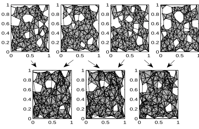
mapping by inclusion intoKti∪Kti+1, as shown in Equation (2.3). Note that the unionKti∪Kti+1 is obtained using the abstract simplicial complexesKti andKti+1 by identifying vertices that corre-spond to the same sensor. For a set ofT snapshots at time pointst1,t2, . . .,tT, we thus obtain the
(Kt1∪Kt2) (Kt2∪Kt3) (KtT−1∪KtT)
Kt1 Kt2 · · · KtT
(2.3)
and the associated zigzag persistence module:
H1(Kt1∪Kt2) H1(Kt2∪Kt3) H1(KtT−1∪KtT)
H1(Kt1) H1(Kt2) · · · H1(KtT)
See Figure 2.6 for Rips complexes of four time points in a dynamic network (top row), with the union complexes used for mapping through (bottom row). From the zigzag persistence module above, the Pers() ={[bj,dj]}containing the lifetimes of the homological features can be
com-puted. At this stage it is worth noting the distinction between homology classes and coverage holes, as well as the lack of a straightforward definition of what a ‘time-varying coverage hole’ is.
One characterization of a time-varying coverage hole is known as an ‘evasion path’, which means that there exists a spatiotemporal path which remains uncovered. This can be thought of as a path that an intruder could travel in order to avoid detection. Homological methods have been used [48]to give necessary conditions for such an evasion path to exist, using the same coordinate-free
homolog-0 0.5 1 0 0.2 0.4 0.6 0.8 1
0 0.5 1
0 0.2 0.4 0.6 0.8 1
0 0.5 1
0 0.2 0.4 0.6 0.8 1
0 0.5 1
0 0.2 0.4 0.6 0.8 1
0 0.5 1
0 0.2 0.4 0.6 0.8 1
0 0.5 1
0 0.2 0.4 0.6 0.8 1
0 0.5 1
0 0.2 0.4 0.6 0.8 1
Figure 2.6Sequence of Rips complexes and their union complexes.
ical features in zigzag persistence can, however, be done unambiguously, and although these are not interpreted as individual time-varying coverage holes, they are related to the coverage region in the following ways:
1. If a coverage hole appears at timeb and remains isolated (does not split or merge with any other holes) until it disappears at timed, then the exact interval[b,d]will be present in Pers(). This means that in the case where a time-varying coverage hole is well defined, its lifetime is exactly represented in the barcode.
2. If an evasion path exists over interval[b,d], then there exists an interval in Pers() contain-ing[b,d]. This means that no evasion paths will be missed.
3. If Pers() = {[bj,dj]| j ∈ 1, . . .,m} are the intervals output from zigzag persistence, then
Then
|Λi|=β1(Ki)
(the number of intervals alive at any time point is equal to the number of holes in the simpli-cial complex at that time).
In light of this, we propose the use of the barcode/persistence diagram from zigzag persistent homology as a descriptor of the coverage of a network over time. In general, more bars and longer bars correspond to worse coverage. Since the computation only requires the Rips complexes (i.e. ad-jacency matrices of the communication graph) at each time point, this measure can be computed without requiring coordinates or distances between the sensors. In particular, summary statistics such as maximum and mean lifetimes of homological features can be computed, in addition to analysis of the barcode/persistence diagram as a whole. Metrics (such as the Wasserstein or bottle-neck distances on persistence diagrams - see[12],[11]) have also been developed to compute pair-wise distances between two persistence diagrams, which allows for quantification of differences between the coverage patterns of multiple time-varying networks.
At present, the only methods[37]available for analyzing coverage in dynamic sensor networks are to measure the coverage directly (using geometric information), and compute the proportion of uncovered area at each time point, or the proportion uncovered over a time interval (including a point as covered if it has been covered at any time during the interval).
2.3.3 Comparing mobility models
We present here some results on how the output from zigzag persistence can be used to character-ize the coverage obtained by different mobility models for dynamic sensor networks. The analysis of coverage properties of mobility models previously used geometric descriptors to derive analyt-ical results about the network, such as the limiting distribution of the nodes, the expected time-until-coverage for uncovered points, or expected proportion of uncovered area[37]. Ours is the first method which can additionally describe the dynamics of the coverage, in terms of the formation, duration, and behavior of coverage holes over time.
The two models we discuss are based on Brownian motion, and straight-line motion. For each of these, it is assumed that the nodes move independently from one another.
2.3.3.1 Mobility patterns: Discrete Brownian and Straight Line
Discrete Brownian: One model used to approximate the random movement of nodes in a large scale
sensor network assumes the moves of each node to be independently and identically distributed (i.i.d.) according to a Brownian motion (eg.[43]). This is modeled in discrete-time by allowing each sensor to move according to a 2-dimensional Gaussian distribution at each time step (with variance proportional to the time increment).
Straight Line: A second commonly-used i.i.d. mobility model has each node choose an initial random direction and velocity, and then proceed (indefinitely) along this course ([36],[37]). In this setting, att =0 each node randomly chooses a directionθ∈[0, 2π)according to some distribution described by fΘ(θ), and randomly chooses a speedv∈[vm i n,vm a x]according to a distribution
de-scribed byfV(v). TypicallyfΘ(θ)andfV(v)are uniform distributions over their respective intervals,
2.3.3.2 Simulations
Simulations were performed in a bounded region[0, 1]2, and for both mobility patterns the initial positions of the nodes were drawn from a uniform distribution over the region. When the move-ment of a sensor causes it to reach the boundary of the region, it bounces off with elastic (billiard-like) collisions, which will cause a change in the direction but not the speed.
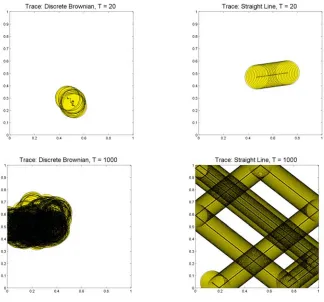
Usingn=100 nodes, over an interval ofT =50 time points, 50 replications were generated for each mobility pattern. The simulations were paired, in that the initial coordinates of the sensors were the same for the two patterns, and were generated independently for each replication. All pairings for computing differences between the patterns, and computing the Wilcoxon signed rank were done by pairing the two replications (one from each mobility pattern) with the same initial configuration of sensors. The 2-dimensional Gaussian distribution used to initialize the movement in Straight Line pattern, and at each time point for the Discrete Brownian, had a mean zero and standard deviation equal to 0.1r (wherer=0.977 is the radius of the coverage disk for each sensor. This was chosen so that the communication graph would have an average degree of 15). A trace of one sensor following each of the mobility patterns forT =20 (top row) and 1000 (bottom row) time points is shown in Figure 2.7, with the Discrete Brownian mobility pattern on the left, and the Straight Line mobility pattern on the right.
For each replication, the sequence ofT simplicial complexesK1, . . .,KT (representing the
sen-sor network at time points 1, . . .,T) are used along with the union complexesKi ∪Ki+1 fori =
1, . . .,T −1 to build the sequence, as in Equation (2.3). This is used as an input to compute the zigzag persistence birth-death intervals Pers() ={[bj,dj]}and associated representative cycles.
A statistical analysis was performed to test for differences in the coverage properties of the two pat-terns, using both traditional coverage measures and descriptors obtained from our homological methods. The variables used for analysis are described in Section 2.3.3.3.
Table 2.1List of the summary statistics extracted from the barcodes.
Variable Description
barcode Anm-by-2 matrix containing the set of birth-death pairs for a given simula-tion run (the numberm will vary, run to run). This is the main descriptor of the tracked homological features using zig-zag persistence.
LTcounts AT-length vector with the counts of how many bars have length (lifetime) t, fort =1, . . .,T in a given simulation run. i.e.)LTcounts(1) is the number of bars that persist for only a single timepoint,LTcounts(2) is the number of bars with a lifetime of 2,. . .,LTcounts(T) is the number of bars that persist over the entire simulation run.
# of bars (scalar) The numberm of birth-death intervals{[bj,dj]| j =1, . . .,m}in a
barcode for a given simulation run.
sum of bars (scalar) The summj=1(dj−bj)of all bar lengths (lifetimes) in a given
simu-lation run.
interval coverage AT-length vector giving the proportion of the simulation region covered by timet, fort =1, . . .,T in a given simulation run. A point in the simulation region is considered covered by time t, if it is covered at any point in the interval[0,t].
[0, 1]2), all point-wise coverage statistics, such as the average proportion of uncovered area or
aver-age number of coveraver-age holes at any time point, should be the same for the two mobility patterns [31]. What we expect might differ between the two groups, is the way in which coverage holes form,
merge, split, and close, which can be detected in differences in the distribution of lifetimes of ho-mology classes (the number and lengths of the intervals in Pers(). i.e. bars in the barcode).
2.3.3.3 Coverage statistics
The output of zigzag persistent homology on the sequence of simplicial complexes gives a set of birth-death intervals Pers() ={[bj,dj]| j=1, . . .,m}for each replication (each represented as a
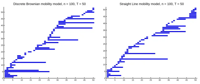
Example barcodes from one simulation run and for each mobility pattern are shown in Figure 2.8 (Discrete Brownian - left, Straight Line - right). The colors of the bars will be later used when identifying bars with specific representative cycles. Note that a quick look at a single pair of bar-codes does not unveil a clear indication of whether there is a difference between the time-varying first homology of the two patterns, thus justifying a more careful statistical analysis. Since the mo-bility patterns are time-stationary, the variables involving the lifetimes of the homological features are of greatest interest, in contrast to those which depend on the specific birth or death time. The statistically insignificant differences in the barcodes led us to look at lifetimes of the homological features.
0 5 10 15 20 25 30 35 40 45 50
0 5 10 15 20 25 30 35 40 45 50
Discrete Brownian mobility model, n = 100, T = 50
0 5 10 15 20 25 30 35 40 45 50
0 5 10 15 20 25 30 35 40 45 50
Straight Line mobility model, n = 100, T = 50
Figure 2.8Barcodes for realizations of Discrete Brownian and Straight Line.
2.3.3.4 Results
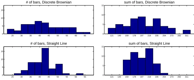
Comparing the Discrete Brownian motion and Straight Line mobility patterns, there is no statis-tically significant difference between the two groups for# of bars[DB=42.42(10.52), SL=42.6(6.42), p=0.70], orsum of bars[DB=201.96(48.19), SL=197.58(25.50),p=0.71]. There is however a statisti-cally significant difference in the variance of the two patterns for both# of bars (p<0.001) andsum of bars (p <0.0001), with the Discrete Brownian pattern having larger variability than the Straight Line. Figure 2.9 shows histograms for the distribution of# of bars (left) and sum of bars (right) for the Discrete Brownian (top row) and Straight Line (bottom row) mobility patterns.
The counts of lifetimes are distributed differently for the two groups. The Discrete Brownian mobility pattern has a significantly higher number of very short lifetimes (fort =1,p <0.0001), and very long lifetimes (fort =50,p <0.001). A few long lifetimes (t =19 and 22) are also more frequent in the Discrete Brownian pattern, with moderate significance (p<0.05). The Straight Line mobility pattern has a significantly higher number of short-medium length lifetimes (t =4, . . ., 13, all have 0.001<p <0.05). Even after a Bonferroni correction for multiple hypothesis testing, the differences fort =1 and 50 are still statistically significant (at the levelp <0.001). Histograms of LTcounts for the two mobility patterns are shown in Figure 2.10, with the lifetimes that show statis-tically significant differences highlighted. The Discrete Brownian (top left) and Straight Line (bot-tom left) mobility patterns, as well as the paired difference inLTcounts(right) are shown, with the lifetimes whose frequency has a statistically significant difference between the groups highlighted. The lifetimes that occur more frequently in the Discrete Brownian pattern (t =1, 19, 22 and ,50) are highlighted in red in the top plot, and those that occur more frequently in the Straight Line pattern (t =4, . . ., 13) are highlighted in green in the bottom plot.
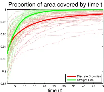
Brownian in red, Straight Line in green). The difference between the two mobility patterns in inter-val coverageis statistically significant for time pointst =7, . . .,T (p<0.001). This is in agreement with previous work[36], as well as the fact that a sensor traveling a path of fixed total length will cover the greatest area if it travels in a straight line. We additionally note that the time-point-wise coverage, measured by proportion of covered area, as expected shows no statistically significant difference between the patterns, see Figure 2.12. Again, all simulation runs are overlaid as dotted lines, with mean coverage shown as a thick, solid line for each mobility pattern (Discrete Brownian in red, Straight Line in green)
25 30 35 40 45 50 55 60 65
0 5 10 15
# of bars, Discrete Brownian
25 30 35 40 45 50 55 60 65
0 5 10 15
# of bars, Straight Line
121 140 159 178 197 216 235 254 273 292 311
0 5 10 15
sum of bars, Discrete Brownian
121 140 159 178 197 216 235 254 273 292 311
0 5 10 15
sum of bars, Straight Line
Figure 2.9Histograms comparing number of bars in two mobility patterns.
2.3.3.5 Discussion
0 5 10 15 20 25 30 35 40 45 50 0
5 10 15
Average Counts of lifetimes, Discrete Brownian
DB > SL
0 5 10 15 20 25 30 35 40 45 50
0 5 10 15
Average Counts of lifetimes, Straight LIne
SL > DB
0 5 10 15 20 25 30 35 40 45 50
−1 0 1 2 3 4 5 6
Difference (DB−SL) in LTcounts
DB > SL (signif) SL > DB (signif)
Figure 2.10Comparison of counts of lifetime lengths for the two patterns.
5 10 15 20 25 30 35 40 45 50
0.88 0.9 0.92 0.94 0.96 0.98 1
time (t)
Proportion of area covered by time t
Discrete Brownian Straight Line
5 10 15 20 25 30 35 40 45 50 0.85
0.9 0.95 1
time (t)
Proportion of area covered at time t
Discrete Brownian Straight Line
Figure 2.12Proportion of area covered over time for the two patterns.
pattern displays significantly more long-lasting coverage holes, which typically correspond to large holes that are present in the initial configuration (i.e. the mobility pattern does not fill in existing holes quickly). For the Straight Line mobility pattern, since the sensors are each following a smooth trajectory, the coverage holes seem to appear, grow, shrink and disappear smoothly, instead of ap-pearing and disapap-pearing rapidly, or remaining uncovered for longer periods. In light of this, the Straight Line mobility model would be preferable in situations such as surveillance, or intruder detection, where it is important to quickly cover holes present in the initial deployment, and long-lasting coverage holes would prove costly. The Discrete Brownian model might be more desirable in circumstances where a thorough inspection takes precedence over time, such as in geographical surveying or environmental monitoring.
2.4
Coordinate-free estimation of hole size
not correspond to a large hole geometrically. Given that our network is described as a sequence of adjacency matrices (describing the simplicial complex at each snapshot, but without coordinate information), the best available estimate is the hop-length of the shortest cycle surrounding a hole. This can be obtained without having to compute the shortest cycle explicitly, by performing a hop-distance filtration on the simplicial complex (at each time point). For a simplicial complexK, the hop distance filtration is a nested sequence of simplicial complexesK1⊆K2⊆. . . defined as fol-lows:
Definition: Thehop distance filtration on a simplicial complexK, performed up to a maximum
hop distance ofm, is a nested sequence of simplicial complexesK1⊆K2⊆. . .Km, defined
induc-tively:
1. K1is the original complexK
2. Khcontains all of the simplices ofKh−1, and adds edges between any nodes that werehhops apart inK, as well as all possible higher-dimensional simplices (i.e. if three edges forming a triangle are present inKh, the associated 2-simplex will be added toKhas well).
1 hop (original complex) 2 hops 3 hops
Figure 2.13Illustration of hop distance filtration.
Hop-length of shortest Persistence of hole in cycle surrounding hole hop distance filtration
4, 5, 6 1
7, 8, 9 2
10, 11, 12 3
..
. ...
3k+1, 3k+2, 3k+3 k
To illustrate the benefit of incorporating hop-distance size estimates, we compare various possi-ble homological descriptors of timepoint-wise coverage with the true geometric coverage informa-tion. This was carried out for each time point in all of the simulation runs for the Discrete Brownian model described in the previous section (for 50×50=2500 points), the results of which are shown in scatterplots in Figure 2.14. The plots shown are: left - first betti number (r =0.176); middle - sum of hole sizes (measured using depth in hop distance filtration,r =0.505); right - sum of squared hole sizes (measured using depth in hop distance filtration,r =0.747). For a given sensor network we measure the geometric coverage by the proportion of total area contained inside the coverage holes (ignoring uncovered area along the boundary of the simulation region, which is undetectable by the simplicial complex), and refer to this measure ascoverage hole area. The homological cov-erage descriptors based on coordinate-free data only are:
1. The number of holes in the complex (first Betti number)
2. The sum of the hole sizes (measured by depth in the hop distance filtration)
3. The sum of the squared hole sizes (i.e. sum of squared depths)
As mentioned above, the number of holes in a simplicial complex (the first Betti number) does not describe the hole sizes at all. By combining information about the number of holes along with their estimated sizes, we are able to obtain a coordinate-free descriptor which correlates well with the true geometric information about the size of the coverage holes. This is rather surprising, since the coordinate-free information is very coarse relative to the geometric.
A note on the computational complexity of performing the hop distance filtration is in order, since the simplicial complexesKh grow large quickly ash increases. The filtration does not
0 1 2 3 4 5 6 7 8 9 10 0 0.01 0.02 0.03 0.04 0.05 0.06 0.07 0.08 (Correlation 0.17979)
Number of holes (β1)
Coverage hole area (proportion)
0 2 4 6 8 10 12 0 0.01 0.02 0.03 0.04 0.05 0.06 0.07 0.08 (Correlation 0.50828)
Sum of hole sizes (hop dist)
Coverage hole area (proportion)
0 2 4 6 8 10 12 14 16 18 20 0 0.01 0.02 0.03 0.04 0.05 0.06 0.07 0.08 (Correlation 0.74768)
Sum of squared hole sizes (hop dist)
Coverage hole area (proportion)
Figure 2.14Coverage hole area vs homological features.
first homology, to increase efficiency of the computations. An alternative method to improve effi-ciency would be to compute persistent homology of the filtration using the Morse theoretic col-lapse algorithm presented in[40].
In addition to using the hop-distance filtration as a measure of the sizes of the holes present in the network at each time point, we would like to link the hole sizes present at timei, with the bars (obtained from zigzag persistence) at timei, for each time pointi. The hop depth information can be combined with the zigzag persistence, to enhance a barcode with estimated size information for each bar at each time point. To that end, we need to make a choice for the homology class corre-sponding to each bar, as well as a specific representative cycle for that homology class. Observing when the inclusion of the cycle becomes trivial in the hop-distance filtration will tell us the size of the largest hole that cycle encircles. Unlike the set of birth-death intervals, the choice of homology class for each bar is not unique, so we would like our choice to be geometrically-motivated, and as close as possible to the ‘canonical basis’ described at the end of Section 2.2.1, thus having each homology class surrounding exactly one hole. The method we propose to achieve this is described in the following section.
subsequent complexes, until the first homology is trivial, will yield the number of holes that are ‘killed’ at each depth. Since the sizes of the complexes grows large quickly ash increases, this can be obtained efficiently by performing a topology-preserving simplicial collapse method[54]before computing the homology.
2.5
Tracking representative cycles
Given the set of intervals{[bj,dj]}obtained from zigzag persistence, we want to have a choice of
representative cycle for each interval, at each time point. The homology classes for this set of cycles should form a basis for the homology, and the choice of representative cycles over time should map into each other in a meaningful way. We propose a method, to be computed alongside the zigzag algorithm, which returns such representative cycles. The method is briefly described here, with a detailed mathematical and algorithmic description reserved for Chapter 3.
Intuitively this method aims to compute a ‘canonical basis’ (described at the end of Section 2.2.1), where there is one representative cycle surrounding each hole. Given the Rips complex for a static sensor network, without an embedding or geometric information, such a canonical basis is impossible to obtain. In the time-varying setting however, a small amount of ‘canonical’ infor-mation is available: when a coverage hole is first formed by the removal of a 2-simplex (triangle), the boundary of that triangle is known to surround exactly the hole of interest. The idea behind our method is then to use that boundary as the representative cycle for the homology class at its birth time, and propagate that information forward through the sequence of complexes as best as possible. The representative cycles we choose need to also be compatible with the interval decom-position in the zigzag algorithm, (the technical detail of this compatibility is described in[21]).
When applying this method alongside the zigzag algorithm, each bar in Pers() ={[bj,dj]}is
avail-able to us. We can obtain size estimates for the hole(s) by including the representative cycle in the hop-distance filtration of the complex (at each time point), as described in Section 2.4. If the rep-resentative cycles did indeed form a canonical basis, then the size information about each hole over time would be attached one-to-one with a corresponding bar. Although guarantees of a true canonical basis are impossible, when implemented in practice the method gives representative cy-cles that are geometrically quite meaningful. Short-lived holes are typically surrounded by a tight cycle at their boundary, and holes that begin with the removal of a triangle and then grow in size are also well-tracked.
2.5.1 Examples
Here, we present a number of examples where the representative cycles and associated size esti-mates give useful and interesting results, unavailable through other methods. Recall that all of the results and computations discussed in this section are obtained using only the communication graph of the network at each time point, with no information about coordinates or distances be-tween neighboring sensors.
2.5.1.1 Tracking holes in a dense network
0 2 4 6 8 10 12 14 16 18 20 0 2 4 6 8 10 12 Barcode
0 0.1 0.2 0.3 0.4 0.5 0.6 0.7 0.8 0.9 1 0 0.1 0.2 0.3 0.4 0.5 0.6 0.7 0.8 0.9 1
Time 7
0 0.1 0.2 0.3 0.4 0.5 0.6 0.7 0.8 0.9 1 0 0.1 0.2 0.3 0.4 0.5 0.6 0.7 0.8 0.9 1
Time 8
0 0.1 0.2 0.3 0.4 0.5 0.6 0.7 0.8 0.9 1 0 0.1 0.2 0.3 0.4 0.5 0.6 0.7 0.8 0.9 1
Time 9
0 0.1 0.2 0.3 0.4 0.5 0.6 0.7 0.8 0.9 1 0 0.1 0.2 0.3 0.4 0.5 0.6 0.7 0.8 0.9 1 Time 10
0 0.1 0.2 0.3 0.4 0.5 0.6 0.7 0.8 0.9 1 0 0.1 0.2 0.3 0.4 0.5 0.6 0.7 0.8 0.9 1 Time 11
0 0.1 0.2 0.3 0.4 0.5 0.6 0.7 0.8 0.9 1 0 0.1 0.2 0.3 0.4 0.5 0.6 0.7 0.8 0.9 1 Time 12
0 0.1 0.2 0.3 0.4 0.5 0.6 0.7 0.8 0.9 1 0 0.1 0.2 0.3 0.4 0.5 0.6 0.7 0.8 0.9 1 Time 13
0 0.1 0.2 0.3 0.4 0.5 0.6 0.7 0.8 0.9 1 0 0.1 0.2 0.3 0.4 0.5 0.6 0.7 0.8 0.9 1 Time 14
0 0.1 0.2 0.3 0.4 0.5 0.6 0.7 0.8 0.9 1 0 0.1 0.2 0.3 0.4 0.5 0.6 0.7 0.8 0.9 1 Time 15
0 0.1 0.2 0.3 0.4 0.5 0.6 0.7 0.8 0.9 1 0 0.1 0.2 0.3 0.4 0.5 0.6 0.7 0.8 0.9 1 Time 16
0 0.1 0.2 0.3 0.4 0.5 0.6 0.7 0.8 0.9 1 0 0.1 0.2 0.3 0.4 0.5 0.6 0.7 0.8 0.9 1 Time 17
0 0.1 0.2 0.3 0.4 0.5 0.6 0.7 0.8 0.9 1 0 0.1 0.2 0.3 0.4 0.5 0.6 0.7 0.8 0.9 1 Time 18
0 0.1 0.2 0.3 0.4 0.5 0.6 0.7 0.8 0.9 1 0 0.1 0.2 0.3 0.4 0.5 0.6 0.7 0.8 0.9 1 Time 19
0 0.1 0.2 0.3 0.4 0.5 0.6 0.7 0.8 0.9 1 0 0.1 0.2 0.3 0.4 0.5 0.6 0.7 0.8 0.9 1 Time 20
2.5.1.2 Detecting and evaluating severity of expanding failure region
In dense networks, the coverage holes are typically small and short-lived, so the representative cy-cles themselves provide fairly accurate tracking. Cases where the representative cycle itself does not ‘tightly’ surround a hole, its inclusion in the hop-distance filtration will still accurately reflect the size of the hole. This is especially useful for holes that are persistent over time, to better understand whether the hole is of increasing severity (perhaps due to a malicious attack or systematic failure). To compute dynamic size estimates for the hole(s) associated with each bar, the persistence in the hop-distance filtration for each representative cycle is attached to its corresponding bar at each time point. This is visualized in the barcode by thickening the bar by an amount proportional to the depth its representative cycle persists in the hop-distance filtration at that time. Figure 2.16 shows snapshots of a time-varying network with an expanding failure region, and the associated thickened barcode is shown in Figure 2.17 (with hop-distance computed up to a maximum depth of 3). It can be seen that the hole which is growing in time is easily observed in the barcode as a bar which thickens over time.
2.5.1.3 Maintaining perimeter around a guarded region
0 0.1 0.2 0.3 0.4 0.5 0.6 0.7 0.8 0.9 1 0 0.1 0.2 0.3 0.4 0.5 0.6 0.7 0.8 0.9 1
Time 6
0 0.1 0.2 0.3 0.4 0.5 0.6 0.7 0.8 0.9 1 0 0.1 0.2 0.3 0.4 0.5 0.6 0.7 0.8 0.9 1
Time 7
0 0.1 0.2 0.3 0.4 0.5 0.6 0.7 0.8 0.9 1 0 0.1 0.2 0.3 0.4 0.5 0.6 0.7 0.8 0.9 1
Time 8
0 0.1 0.2 0.3 0.4 0.5 0.6 0.7 0.8 0.9 1 0 0.1 0.2 0.3 0.4 0.5 0.6 0.7 0.8 0.9 1
Time 9
0 0.1 0.2 0.3 0.4 0.5 0.6 0.7 0.8 0.9 1 0 0.1 0.2 0.3 0.4 0.5 0.6 0.7 0.8 0.9 1 Time 10
0 0.1 0.2 0.3 0.4 0.5 0.6 0.7 0.8 0.9 1 0 0.1 0.2 0.3 0.4 0.5 0.6 0.7 0.8 0.9 1 Time 11
0 0.1 0.2 0.3 0.4 0.5 0.6 0.7 0.8 0.9 1 0 0.1 0.2 0.3 0.4 0.5 0.6 0.7 0.8 0.9 1 Time 12
0 0.1 0.2 0.3 0.4 0.5 0.6 0.7 0.8 0.9 1 0 0.1 0.2 0.3 0.4 0.5 0.6 0.7 0.8 0.9 1 Time 13
0 0.1 0.2 0.3 0.4 0.5 0.6 0.7 0.8 0.9 1 0 0.1 0.2 0.3 0.4 0.5 0.6 0.7 0.8 0.9 1 Time 14
0 0.1 0.2 0.3 0.4 0.5 0.6 0.7 0.8 0.9 1 0 0.1 0.2 0.3 0.4 0.5 0.6 0.7 0.8 0.9 1 Time 15
0 0.1 0.2 0.3 0.4 0.5 0.6 0.7 0.8 0.9 1 0 0.1 0.2 0.3 0.4 0.5 0.6 0.7 0.8 0.9 1 Time 16
0 0.1 0.2 0.3 0.4 0.5 0.6 0.7 0.8 0.9 1 0 0.1 0.2 0.3 0.4 0.5 0.6 0.7 0.8 0.9 1 Time 17
0 0.1 0.2 0.3 0.4 0.5 0.6 0.7 0.8 0.9 1 0 0.1 0.2 0.3 0.4 0.5 0.6 0.7 0.8 0.9 1 Time 18
0 0.1 0.2 0.3 0.4 0.5 0.6 0.7 0.8 0.9 1 0 0.1 0.2 0.3 0.4 0.5 0.6 0.7 0.8 0.9 1 Time 19
0 0.1 0.2 0.3 0.4 0.5 0.6 0.7 0.8 0.9 1 0 0.1 0.2 0.3 0.4 0.5 0.6 0.7 0.8 0.9 1 Time 20
0 5 10 15 20 0
1 2 3 4 5 6 7 8 9 10
Barcode weighted by hop persistence
Figure 2.17Weighted barcode for expanding failure region.
2.6
Conclusions and Future Work
We have presented strategies of exploiting computational topology to describe time-varying cover-age in a dynamic sensor network, while using only local information about which nodes neighbor each other at each time step.
Zigzag persistent homology takes the sequence of simplicial complexes (representing the dy-namic network), and outputs a barcode of birth and death times of homological features in the sequence. We described the relationship between these birth-death intervals and the time-varying coverage holes in the network, and demonstrated how the barcode output is a useful quantitative descriptor to detect coverage differences when comparing sensor network mobility patterns.
We developed a method to obtain a specific set of geometrically-meaningful representative cy-cles for each birth-death interval, at each time point. This set of representative cycy-cles is then used to track coverage holes over time, as well as to obtain size estimates (in conjunction with a hop-distance filtration) for the holes at each time point. This size information is then incorporated into the barcode, for a more complete description of the dynamic coverage of the network. While this method was developed with applications to dynamic sensor networks in mind, the algorithm may be also adapted to obtain an adaptive choice of representative cycles in any dimension, for any persistent homology or zigzag persistent homology computation, thus providing an area for future research.
3
ADAPTIVE TRACKING OF
REPRESENTATIVE CYCLES IN ZIGZAG
PERSISTENT HOMOLOGY
For the article this chapter is based on, see[21]or arXiv:1411.5442.