5
REAL-TIME SHADOW CASTING
USING FAKE SOFT SHADOW
VOLUME
Lee Kong Weng, Daut Daman
INTRODUCTION
Shadows are essential to realistic and visually appealing images, but they are difficult to compute in most display environments especially in computer games. Since the introduction of shadow volume by Crow (1977), shadow map by William (1978) and then fake shadows by Blinn (1988, 1996), a lot of development has been done to improve shadow algorithm in real-time graphic application. Current issues about shadow are on real-time dynamic soft shadows and hardware improvement that improvised real-time shadow generation.
RELATED WORK
The pioneer of the shadow research was initiated by Frank Crow in 1977-title of the research paper is Shadow Algorithm’s for Computer Graphics. The proposed method explicitly clips shadow geometry to the view frustums, generating perfect caps where the volume crosses a clipping plane. The improvised version of the Crow’s original algorithm was suggested by Heidmann (1991), where stencil buffer has been added to support the original algorithm. Stencil shadows belong to the group of volumetric shadow algorithm as the shadowed volume in the scene is explicit in the algorithm.
In the year 2000, Carmack suggested a slightly different approach which entails that the view rays are traced from infinity towards the eye. This may stop when encountering the pixel on the geometry that is closest to the eye (Carmack 2000). This reversal of the view rays' direction has given the algorithm the name Carmacks reverse. The two different approaches have also been named zpass and zfail, as the stencil buffer in the original algorithm is changed only when a fragment passes the z-test.
shader and let the texture handle do the clipping. The only setback using this technique is that it limited to spherical shaped light source.
ALGORITHM
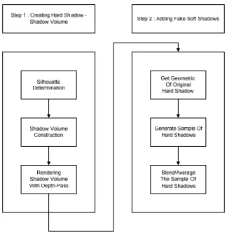
This method combines the existing stencil shadow volume method with Heckbert and Herf soft shadow technique which was originally used for shadow map. This algorithm will be divided into two important steps as shown as Figure 5.1.
Step 1: Creating Hard Shadow Volume
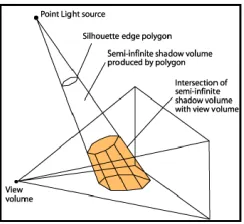
A shadow volume for an object and light is the volume of space that is shadowed. The first step is to create the shadow volume using the silhouette edges of shadowing object/occluder as seen by the light source. After that, the edges are then extruded away from the light and form polygons such as shown by Figure 5.2.
Figure 5.2 Silhouette edge
Figure 5.3 Shadow volume clipping with view volume
Assume the eye is not in shadow, along a ray from the eye, we can track the shadow state by looking at the intersections of shadow volume boundaries. The following rules are applied to track the shadow:
x Each time the ray crosses a front facing shadow polygon, add one to a counter
x Each time the ray crosses a back facing shadow polygon, subtract one from a counter
x Places where the counter is zero are lit, others are shadowed
The algorithm to implement stencil shadow volumes is summed up as (Hun Yen Kwoon 2002):
[1] Render all the objects using only ambient lighting
[2] Starting with a light source, clear the stencil buffer
and calculate the silhouette of all the occluders with respect to the light source.
[3] Extrude the silhouette away from the light source to
an infinite distance to form the shadow.
[4] Render the shadow volumes using the depth-pass.
[5] Using the updated stencil buffer, do a lighting pass
to shade the fragments that corresponds to non-zero stencil values (make it a tone darker).
[6] Repeat step 2 to 5 for all the lights in the scene.
From the above list of steps, it is clear that number of light is in proportion with the frame rate intensity. In fact, the algorithm has to be very selective when deciding which light should be used for casting shadows.
Silhouette Determination
The very first step to construct a shadow volume is to determine the silhouette of the occluder. The stencil shadow algorithm requires that the occluders be closed to triangle meshes. This means that every edge in the model must only be shared by two triangles thus avoiding any holes that would expose the interior of the model. There are many ways to calculate the silhouette edges and each of them are highly computation.
in the cyclic chain 1ĺ2ĺ3ĺ1. The indexes i1,i2 and i3are ordered such that the positions of the vertices Vi1,Vi2 and Vi3 to which they refer are twist counter clockwise about the triangles normal vector. Suppose that two triangles share an edge whose endpoints are the vertices Va and Vb. The consistent winding rule enforces the property that for one of the triangle faces, the index referring to Va precedes the index referring to Vb and that for the other triangle, and the index referring to Vb precedes the index referring to Va.
With this, the edges of a triangle mesh can be identified by making a single pass through the triangle face list. For any triangle having vertex indexes i1, i2 and i3, create an edge record for every instance in which i1ĺ i2,
i2ĺ i3, andi3ĺ i1 and store the index of the current triangle
face in the edge record. Once all the edges are identified, make a second pass through the triangle face list to find the second triangle that shares each edge. This is done by locating triangles for which i1ĺ i2, i2ĺ i3, or i3ĺ i1 and
matching it to an edge having the same vertex indexes that has not yet been supplied with a second triangle index. The general concept of this explanation can be expressed using the following pseudo code:
1. for each triangle face (A) in the object/model 2. for each edge in A
3. if this edge triangle face (neighbors)is not known yet
4. for each triangle face (B) in the object/model except A
5. for each edge in B
for each triangle face A and B, then move onto next edge in A
With the edge list for a triangle mesh/face, the silhouette is determined by substituting the light position with the plane equation. A triangle face that is visible to light source will have a value of plane equation > 0. The silhouette is equal to the set of edges shared by a visible triangle and a triangle face that is not visible to the light. This is done by examining all the triangle faces and checking the visible edges. The edge where there is no neighboring triangle face or the neighboring triangle face is not visible to light source will be the silhouette and it casts shadow.
It is important to note that silhouette determination is one of the two most expensive operations in stencil shadow volume implementation. The other is the shadow volume rendering passes to update the stencil buffer. These two areas are prime candidates for aggressive optimizations.
Shadow Volume Construction
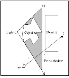
extruded to “infinity” in order to avoid the awkward situation where the light source is very close to an occluder. If that happens [see the illustration shown in Figure 5.4], finite shadow volume extrusion fails to cover all the shadow receivers in a scene.
Figure 5.4 Finite shadow volume fails to shadow
other objects
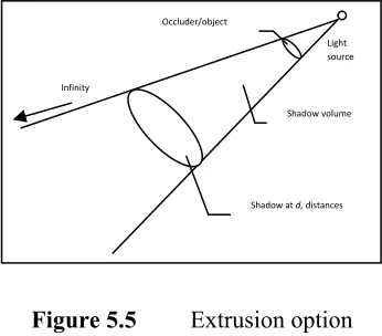
Figure 5.5 Extrusion option
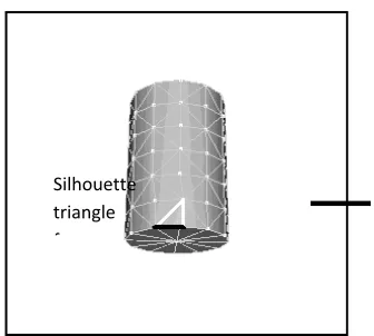
The next procedure is to determine the triangle faces that are visible to light source. The procedure will provide a triangle face that is situated at the edge of the silhouette. A triangle face with no neighboring triangle face, or the neighboring triangle face which is not visible to the light source (refer Figure 5.6), and is called silhouette triangle face from now on.
Occluder/object
Shadowvolume
Shadowatd,distances Infinity
Light
Figure 5.6 The edge for casting shadow volume
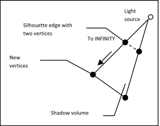
In order to obtain the edge that are at silhouette (the black line edge), edge test need to be done in which a single silhouette triangle face is colored with black and white line (Figure 4.6). The single edge will provide two vertices, which will be used to extrude to another two vertices that will be generated. A basic scaling transformation is applied to extrude the shadow volume by using the two vertices at the silhouette edge. The extrusion process will produce new vertices and they need to be projected along the vector between the light source and the first silhouette edge. It is than scaled to INFINITY value - set to a very large value (refer Figure 5.7).
Silhouette
triangle
Figure 5.7 Extruding to INFINITY by producing two new
additional vertices
The scaling transformations to produce the new vertices are shown as:
x f
f x x s
x
x' ( )
y f
f y y s
y
y' ( )
z f
f z z s
z
z' ( )
Vertices P’(x’, y’, z’) is a new vertex, L(x, y, z) is the light source location, and O(x, y, z) is the vertex from the silhouette edge. By using the above equations two new vertices are produced (illustrated as black color normal line in Figure 5.7) while the other vertices are illustrated as black color dash line. The generated vertices are than used to form the quadrilateral which is needed to create the shadow volume. After creating the shadow volume the
Silhouetteedgewith
twovertices
New
vertices
Shadowvolume
Light
source
next process is to render it, so that the hard shadow is visible.
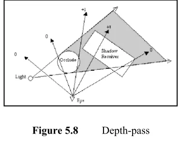
Rendering Shadow Volume Using Depth-Pass
Figure 5.8 Depth-pass
the stencil buffer with the back faces (“turning off” the shadow between the object and any other surfaces).
Once shadow volumes have been rendered for all objects that could potentially cast shadows into the visible region of the scene, it will later cause all the areas that are in shadow volume to have a non-zero stencil value while all those areas in the light area remain zero. Lighting pass are performed to illuminates surfaces wherever the stencil value remain zeroes, re-enable writes to the color buffer, change the depth test to pass only when fragment depth values are equals or less to those in the depth buffer and configure the stencil test to pass when the value in stencil buffer is not equal to zero. Then, draw the blended onto the screen that will cast the hard shadow. The technique is known as depth-pass technique since it manipulates the stencil values only when depth test passes. The following is the general overview of the algorithm;
[1] Render front face of shadow volume. If depth test
passes, increment stencil value, else do nothing. Disable draw to frame and depth buffer.
[2] Render back face of shadow volume. If depth test
passes, decrement stencil value, else do nothing. Disable draw to frame and depth buffer.
Step 2: Adding Fake Soft Shadow
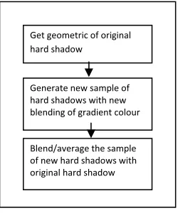
technique was implemented interactively by exploiting graphics workstation hardware. Since hardware has become more affordable and computationally fast, the technique is feasible to be implemented on desktop computer with a standard graphic cards. The proposed algorithm is developed by methodically addressing the fundamental limitations of the conventional stenciled shadow volume. The approach towards soft shadow uses the same approach taken by earlier researcher. The workflow of adding soft shadow for hard shadow volume is shown at Figure 5.9.
Figure 5.9 Work flow for adding soft shadows
Get Geometric of the Original Hard Shadow
The very first step in generating the soft shadows is to get the geometric of hard shadows generated earlier. This can be done by saving all the generated coordinates of the
Getgeometricoforiginal
hardshadow
Generatenewsampleof
hardshadowswithnew
blendingofgradientcolour
Blend/averagethesample
ofnewhardshadowswith
vertices generated while rendering shadow volume in depth-pass technique so that no calculation will need to be done again. This will save computation cost.
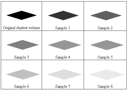
Generate Sample of Hard Shadows
Sample of hard shadows can be generated using blending of gradient colors and can be done by drawing the same shadow geometric volume (refer to Figure 5.10). However, this time the size of the shadow volume polygon is scaled, so that it is slightly bigger than the original shadow volume. The amount of sample depends on the quality of soft shadows.
Generating the sample of hard shadows as shown in Figure 5.10 does not take a lot of processing time rendering. Here, the selection of number of samples must be taken into consideration so that it will not slow down the frame rate. The quality of the soft shadow depends on the amount of the generated samples- the more the better. However, this will increased CPU consumption and performance.
Blend/Average The Sample Of Hard Shadows
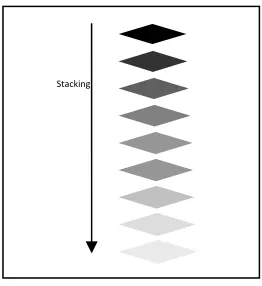
The last step of adding fake soft shadows is to blend or average out the samples together with the original shadow volume. The illustration on how the stacking of the sample can be view on Figure 5.11.
Figure 5.11 Stacking of the sample and original shadow
volume
The production of stacking the sample and original shadow volume must be done from the less dark sample to the darkest in order to produce a new shadow which is a soft shadow. The produced soft shadow will have penumbrae effects on the edge of shadow, which differ from the original shadow volume that has only the hard shadow (Refer Figure 5.12 for illustration).
Figure 5.12 Comparison of original shadow volume and new
softshadow volume
Figure 5.13 Length and gap factor
RESULTS
To actually implement the technique discussed so far in this research can be a daunting task with lots of potential pitfalls and problems. In this section, the implementation and some of the testing details were presented for clarity reasons. Since one of the main goals with this research was to test the applicability of soft shadow in a true 3D environment, the implementation and testing were done with complex and high polygon model. The method used to determine an accurate shadow that resembles real life shadow was side-by-side visual comparisons with reference examples. The approach was also applicable to measure the quality of the produced fake soft shadows. Speed comparisons were performed by observing the frame rate and also by using the reported results of other algorithms. The running time of the algorithms depends on factors such as the screen resolution, the number of polygon, desired quality, graphics hardware and CPU speed. The first test was Accuracy or Resemblance Test. It is to test the accuracy of the shadow produced whether it resembles the real life shadows. Quality Test is performed next on soft
Length
factor
Gapfactor Original
hard
shadow
Samplehard
shadow
shadows qualities. Finally Real-Time Test is done to test the speed of the shadow generation.
Accuracy or Resemblance Test
The shadows generated by the prototype are guaranteed true, real and accurate shadow because it uses the model or shadow caster geometric to produce the shadow. There is no model simplification done to optimized rendering. The produced shadow in this prototype is real, true and accurate or resemble the model/shadow caster (refer Figure 5.14).
Figure 5.14 Research prototypes featuring true, real and
accurate or resemble the model/shadow caster
Quality Test
parameter of length and gap factor. The test result images are captured and the numbers of polygon triangles produced are recorded. Later, the comparison and analysis is done to evaluate the quality of the soft shadow produced, as shown at Figure 5.15.
Figure 5.15 Test results using Cube with different length and
gap
The next test is done by visually comparing the shadow images rendered by our result with another soft shadow volume algorithm developed by Assarson and Akenine-Möller (2003). The experiment involves a cube and sphere in a simple environment. From the experiment, it is seen that the prototype was able to render at about 60 FPS but the quality is poorer. The illustrations of the comparison are shown in Figure 5.16.
Real-Time Test
One way to obtain a fast soft shadow algorithm is to utilize the graphics hardware. Shadow volume consumes a lot of CPU and GPU processing because it requires a lot of computation especially in silhouette edge determination and two pass rendering. Speed comparison was also performed against Assarson and Akenine-Möller’s (2003) algorithm and as well as other algorithms.
Figure 5.17 FPS vs. model polygon count for 3 different
systems using Fake Soft Shadow Volume with Stencil Buffer
FPS vs Model Polygon Count For 3 Different Systems Using Fake Soft Shadow Volume With Stencil Buffer
0.00 100.00 200.00 300.00 400.00 500.00 600.00
0 200 400 600 800 1000 1200 1400 1600 1800
Model Polygon Count
FP
S
These tests were meant to generally test each soft shadow algorithm against three different systems to determine the best setting. The result shows that the qualities of the soft shadows are almost identical in particular with the value of 3.0 for length and 0.3 for gap. The environment was set to 800x600 with 32 bit colours. This is to ensure that the same amounts of polygon are used to render the soft shadow so that a proper comparison can be carried out. Figure 5.17 shows the graph of test using the research prototype that implements the “Fake Soft Shadow Volume with Stencil Buffer” and “Approximate Soft Shadow On Arbitrary Surfaces Using Penumbra Wedge”.
Figure 5.18 FPS vs. model polygon count for 3 different
systems with Approximate Soft Shadows on Arbitrary Surfaces Using Penumbra Wedges algorithm
CONCLUSION
In this Chapter, we have shown we have discussed the algorithm to generate an accurate hard shadow volume and to add fake soft shadow onto it. We can get high quality of soft shadow in real-time by using the proposed algorithm. Although the soft shadow is not geometrically accurate as compared to the hard shadow, it resembles penumbrae (soft shadow). This algorithm can be further improved and implemented using programmable graphics hardware to achieve real-time performance. One of the drawback is that the soft shadows effect only involve the planar/surfaces. The future research direction is to explore on how to extend the effect of shadows onto other surfaces and objects in the scene beside the planar.
FPS vs Model Polygon Count For 3 Different Systems With Approximate Soft Shadows on Arbitrary Surfaces Using Penumbra Wedges
0 20 40 60 80 100 120 140
0 200 400 600 800 1000 1200 1400 1600 1800
Model Polygon Count
FP
S
REFERENCE
Eric Haines, 2001, “Soft Planar Shadows Using Plateaus”, Journal of Graphics Tools 6, 1, pp. 19-27.
CASS EVERITT AND MARK J. KILLGARD, March 2002.
Practical and Robust Stenciled Shadow Volumes for Hardware-Accelerated Rendering. Technical Report, NVIDIA Cooperation. Published online at http://www.developer.nvidia.com.
ERIC LENGYEL, 2002. “The Mechanics of Robust Stencil
Shadows”, Gamasutra.com.
FRANK CROW, “Shadow Algorithms for computer
graphics”, Computer Graphics (SIGGRAPH 1977), 11(3), pp. 242-248, 1977
HUN YEN KWOON, 2002. “The Theory of stencil shadow volumes”, GameDev.net.
JIM BLINN, “Me and My (Fake) Shadow,” IEEE Computer Graphics and Applications, vol. 8, no. 1, pp. 82-86, January 1988.
JIM BLINN, 1996. Jim Blinn’s Corner: A Trip Down the Graphics Pipeline, Morgan Kaufmann Publishers, Inc., San Francisco.
JOHNCARMACK, 2000. Unpublished correspondence. KASPER FAUERBY AND CARSTEN KJAER, 2003. “Real-time
Soft Shadows in a Game Engine”, Master’s Thesis.
LANCEWILLIAMS, August 1978. Casting Curved Shadows
on Curved Surfaces. Computer Graphics, Volume 12,
Number 3.
TIM HEIDMANN, 1991. “Real Shadows, Real Time”, Iris
TOMAS AKENINE-MOLLER AND ULF ASSARSSON, 2002.
Approximate soft shadows on arbitrary surfaces using penumbra wedges. In Proceedings of the 13th
Eurographics workshop on Rendering, pages
297-306. Eurographics Association.
Ulf ASSARSSON AND TOMAS AKENINE-MOLLER, 2003. A geometry-based soft shadow volume algorithm using graphics hardware. ACM Transactions on Graphics
(TOG), 22(3):511-520.
ULF ASSARSSON, MICHAEL DOUGHERTY, MICHAEL
MOUNIER, AND TOMAS AKENINE-MOLLER, 2003. An optimized soft shadow volume algorithm with real-time performance. In Proceedings of the ACM
SIGGRAPH/EUROGRAPHICS conference on Graphics