Evolution of growth density equation by constraints on
effective Newtonian constant
G
e f f
Abraão J.S. Capistrano
1,2∗The acceleration of the universe is described as a con-sequence of the extrinsic curvature of the space-time embedded in a bulk space, defined by the Einstein-Hilbert. Using the linear approximation of Nash-Green theorem, we obtain the related perturbed equations in which just the gravitational-tensor field equations con-tribute to propagation of cosmological perturbations. In accordance with Big Bang Nucleosynthesis and solar constraints, we calculate numerically the effective New-tonian functionGe f f to constrain the related
parame-ters of the model. We numerically solve the growth den-sity equation for two possible family of solutions leading to an interesting overdensity and, in some cases, a mild damping of the growth profiles, with a top amplification of the growth perturbations around14%in compari-son withΛCDM model and quintessence. The effective gravitationalΦand Newtonian curvatureΨare also analysed showing mild perturbations in early times in-duced only by the extrinsic curvature differently from theΛCDM standards.
1 Introduction
In the last decades, the dark energy problem turns one of the central debates on the contemporary physics. Follow-ing Occam’s razor principle, the simplest explanation for the observed accelerated expansion of the universe lies within theΛCDM paradigm that invariably leads to the concept of dark energy: an exotic fluid with negative pres-sure that drives the universe to speed up. The paradigm reveals still unanswered questions about the underlying physics or in the lack of a fundamental principle or a definite observational evidence that justifies/proves the existence of the Cold dark matter and the relevance of the cosmological constantΛ. The nature of the cosmological constant is also a problem of its own with the coincidence problems (on the reason of why the matter distribution
andΛ-dark energy content are seen today as the same order of magnitude) and fine-tuning issues. From the semi-classical Einstein’s equations, quantum field theory suggests that the vacuum states of quantum fields con-tribute to a non-zero, constant energy densityρv ac, which
produces an on going perturbation of the gravitational field in cosmology or, equivalently, in the space-time met-ric. References on these problems can be found in [1–7]. Notwithstanding theΛCDM model responds positively to a vast observational evidences of accelerating expansion of the universe [8–20], it does not explain the observed dwarf galaxy populations in the Local group [21–23] and the CDM simulations lead to a discrepancy of the size of a dark matter halo core in comparison with the observed scale length of the galactic disk due to sub-galactic central
cuspstructures [24–28]. For a review at small scale prob-lems within theΛCDM paradigm, see Ref. [29]. We also add the 2-σtension in theσ8-contours of growth of r.m.s
fluctuations on the scale of 8h−1Mpc with a mismatch of
the data inferred from Planck Cosmic Microwave Back-ground (CMB) radiation and Large Scale Structure (LSS) observations withinΛCDM background, which might be a result from systematics or due to deviations of gravity [30]. The problem persists even if one does not consider the Planck CMB data [31] and other evidences indicate similar tensions in the matter distributions around 2-σ [20, 32–34].
The lack of robust solutions from the aforementioned problems led to alternative models to the standardΛCDM, for instance, the dark energy models [35–37], the mod-ified gravity models that change the standard General Relativity (GR) such as F(R) and variants [38–47] and ref-erences therein. In a different direction, we have inves-tigated the embedding of geometries and their conse-quences to a physical theory in a different approach as compared with extra-dimensions models on superstrings
∗ Corresponding author E-mail: [email protected]
1 Federal University of Latin-American Integration, Foz do Iguassu-PR, 85867-670, Brazil
1
or M theories inspired, such as Randall-Sundrum brane-world cosmology and variants [48–50]. In particular, the Randall-sundrum model uses the algebraic Israel- Lanc-zos boundary condition as a relation between the extrinsic curvature and the material sources. The theoretical conse-quence is that the application of such condition does not follow the evolution of the embedded geometry [51]. In this paper, apart from the braneworld context, we study the consequences when considering the universe as an embedded space-time dynamically evolving by pertur-bations of the Nash-Greene embedding theorem [52, 53]. Based on the model proposed in [54–57], we tested the model at background level in a series of previous works [58–62]. Specifically it passed through the cosmokinetics diagnosis, as shown in Ref. [58, 61]. We follow this direc-tion going further on the context of cosmological pertur-bations. In this sense, we intend to propose a relevance of a renewed concept of Riemmanian curvature with the addition of the extrinsic curvature and the Nash-Greene embedding theorem as an oriented mathematical ground.
The outline of paper is as follows. In the section 2 we present a summary of the embedding process present-ing the field equations. Uspresent-ing the linear approximation of Nash-Green theorem, it is shown the background cos-mological equations in compliance with erstwhile pub-lished results [57, 58, 61]. We also investigate the Fried-mann equation modified by extrinsic curvature that de-tains two possible signatureΓ±-solutions and we study a family of these solutions for allowed values of the param-eters. In the section 3, we obtain the perturbed equations in a conformal Newtonian frame and the related growth of contrast matter. To solve the growth equation, we numeri-cally study the effective Newtonian Gravitational constant
Ge f f to obtain a constraint on the parameters. Hence, a numerical analysis is made on the growth equations in comparison withΛCDM model and GR quintessence. The effective gravitationalΦand Newtonian curvatureΨare also analysed. Final remarks are made in the conclusion section.
2 The universe as an embedded space
In this paper we use the same theoretical background of a series of previous works [54–62] in which is possi-ble the description of dynamical embedding without any junction conditions unlike that of rigid embedding mod-els [48, 49]. A common bottom line between braneworld models and other embedding models (this works is an example) is the embedding itself and how to define the dynamics of extrinsic curvature once the embedding can
be made in several different forms (e.g., local or global, isometric, analytic or differentiable etc.). It is important to point out that the junction conditions are not unique [63–67] leading to different physical results [68] and they can be completely ignored depending on the related em-bedding framework such as the seminal works of Arkani-Hamed, Dimopoulos and Dvali, commonly known as ADD model [69] or the DGP model, as an acronym for Dvali, Gabadadze and Porrati’s model [50]. In this work, we use the Nash-Greene differentiable embedding [52, 53] as a principle for dynamical embedding.
2.1 The Nash-Greene embedding process
The main result of the Nash-Greene embedding theo-rem [52, 53] is applicable to an arbitrary number of di-mensions. It shows that the evolution of any embed-dedn-dimensional Riemannian geometryVn in an
N-dimensional larger geometry (bulk) is possible by a se-quence of infinitesimal perturbations of a non-perturbed background metric ˜gµνgiven by the non-perturbed ex-trinsic curvature tensor ˜kµνa. In the case of interest, in a five dimensional bulkV5, the embedding of a four dimen-sional space can be given by the mapX :V4→V5. The fluctuations ofV4lead to a new (perturbed) geometrygµν
gµν=g˜µν+δyk˜µν+(δy)2gρσk˜µρk˜νσ· · ·
and one can obtain linear Nash fluctuations as
δgµν= −2 ˜kµνδy, (1)
whereδydenotes an infinitesimal displacement of the extra dimensionyin the bulk space and it is not consid-ered in the line elements as in the case of rigid embedding models [48, 49]. A similar expression of Eq.(1) was ob-tained year latter after Nash’s seminal work in the ADM quantization program [55]. Since the extension to Pseudo-Riemannian manifolds was made by Greene [53], hereon we refer as Nash-Green theorem. Concerning notation, we adopt the Landau time-like convention (− − −+) for the signature of the four dimensional embedded metric and speed of lightc=1. Capital Latin indices run from 1 ton. Small case Latin indices refer to the only one extra dimension considered. All Greek indices refer to the em-bedded space-time counting from 1 to 4. Non-perturbed quantities are denoted by the tilde symbol.
One can define the actionSas
S= − 1 2κ25
Z p
|G|5Rd5x− Z
p
|G|Lm∗d5x, (2)
whereκ25is the energy scale on the embedded space,5R denotes the five dimensional Ricci scalar of the bulk and
L∗
mdenotes the confined matter Lagrangian. Thus, the
variation of Einstein-Hilbert action in Eq.(2) with respect to the bulk metricGABleads to the Einstein equations for
the bulk
5R AB−
1
2GAB=α ?T
AB, (3)
whereα?is the energy scale parameter andTAB is the
energy-momentum tensor for the bulk [54–57].
This model can be regarded as a four-dimensional hypersurface that evolves in a five-dimensional bulk with constant curvature whose related Riemann tensor is
5R
ABC D=K∗(GACGB D−GADGBC) , A..D=1· · ·5 ,
whereGAB denotes the bulk metric components in
ar-bitrary coordinates. In five dimensions, we can write in embedded vielbein {Z,Aµ,ηA} for the metric of the bulk in
the vicinity ofV4
GAB = Ã
˜
gµν0 0 1 !
. (4)
The perturbed coordinateZAis given by the Lie transport
Lsuch as
ZA
,µ=X,µA+δy LηXA
,µ=X
A
,µ+δyηA,µ, (5)
ηA=ηA+δy[η,η]A =ηA. (6)
and the normal vector isηAunspoiled by perturbations [54–56].
It is worth noting that the constant curvatureK∗is either zero (flat bulk) or it can have positive (de Sit-ter) or negative (anti-de SitSit-ter) constant curvatures. We chose a flat bulk withK∗=0. The confined tangent com-ponents of the energy-momentum tensor for the bulk TAB are proportional to the energy-momentum tensor: α∗Tµν=8πGNTµν, whereGNis the gravitational
Newto-nian constant. On the other hand, the vectorTµa and scalar Tab components are confined in the sense that Tµa=0 andTab=0 prohibit any propagation of matter
fields to extra-dimension, but the gravitational field. The field equations can be obtained by direct calcu-lation of the tangent components of Eq.(3). As shown in details in Refs.( [54–57]) one can write the induced field equations in the embedded space-time from a five-dimensional bulk
˜
Gµν+Q˜µν =8πGNT˜µν, (7)
˜
kµ[ν;ρ]=0 , (8)
where the energy-momentum tensor of the confined per-fect fluid is denoted by ˜Tµν. The quantity ˜Gµνdenotes the
four dimensional non-perturbed Einstein tensor and ˜Qµν
is thedeformation tensor. This term is defined by
˜
Qµν=g˜ρσk˜µρk˜νσ−k˜µνh˜2−1 2
¡˜ K2−h˜2¢
˜
gµν, (9)
where we denote ˜h2=h˜. ˜hby the mean Gaussian curva-ture and ˜K2=k˜µνk˜µνdenotes the Gaussian curvature. It follows that ˜Qµνis a conserved quantity in the sense that
˜
Qµν;ν=0 . (10)
We point out that the trace of the Codazzi equation in Eq.(8) is composed by the extrinsic curvature terms and the appearance of the deformation tensor ˜Qµνof Eq.(9) are a novelty typically inherent to embedding models that extend the curvature concept of a pseudo-Riemannian ge-ometry. The brackets in Eq.(8) apply the covariant deriva-tives to the adjoining indices.
To complete the set of dynamical equations, the ex-trinsic curvature dynamics is completed by the analysis of the spin of a linear massless spin-2 fields in Minkowski space-time. Counting from Eq.(3), one obtains a total of 20 unknowns ˜gµν and ˜kµν, against 15 dynamical equa-tions. Thus, the remaining equations must come from ˜kµν
which is an independent symmetric rank-2 tensor. In 1954, Suraj Gupta noted that the Fierz-Pauli equation has a re-markable resemblance with the linear approximation of Einstein’s equations for the gravitational field, suggesting that such equation could be just the linear approximation of a more general, non-linear equation for a massless spin-two fields. Gupta found that any spin-2 field in Minkowski space-time must satisfy an equation that has the same for-mal structure as Einstein’s equations [70–73]. As a result, a set of Einstein-like system of equations called the Gupta equations that are defined as a Ricci-like equations in a form
˜
Fµν=0 , (11)
where they are defined as a copy of the usual Riemannian geometry. Hence, once can define a “f-Riemann tensor”
˜
Fµναλ= ∂αΥµλν−∂λΥµαν+ΥασµΥσλν−ΥλσµΥσαν
constructed from a “connection” associated with ˜kµν. It is worth noting that this is not a bimetric model likewise Rosen Bimetric theory [74] since the true background geometry of the embedded space-time is defined by the metric tensor ˜gµν. Thus, we define the tensors
˜
fµν= 2˜
K
˜
kµν, and ˜fµν= 2˜
K
˜
kµν, (12)
so that the normalization condition ˜fµρf˜ρν =δµν is
ap-plied and ˜K = q
˜
kµνk˜µν. Accordingly, it is possible to
define the “Levi-Civita connection” associated with ˜fµν, based on the analogy with the “metricity condition”
˜
fµν||ρ=0, where the double bars||denote the covariant derivative with respect to fµν (while keeping the usual semicolon sign for the covariant derivative with respect to ˜gµν). The “f-connection” is given by
Υµνσ= 1 2 ¡
∂µf˜σν+∂ν f˜σµ−∂σf˜µν¢
and also the contraction
Υµνλ=f˜λσΥµνσ.
2.2 Background FLRW embedded universe
In order to describe the cosmological background, we use Eqs.(7), (8) and (11), with the usual Friedman-Lemaître-Robertson-Walker (FLRW) in coordinates (r,θ,φ,t)
d s2= d t2−a2£
d r2+fκ2(r)¡
dθ2+sin2θdϕ2¢¤
, (13)
wherea=a(t) is the scale expansion factor,f(r)κ=sinr, r,sinhrandκcorresponds to spatial curvature (1, 0,−1). For the present application, we consider a flat universe.
The stress energy tensor in a non-perturbed co-moving fluid with a co-co-moving velocityuµ is given by
˜
Tµν=¡ ˜
ρ+p˜¢
uµuν−p˜g˜µν;uµ=δ4µ. (14)
The related conservation equation
˜
ρ+3H¡ ˜
ρ+p˜¢
=0 , (15)
where ˜ρand ˜pdenote non-perturbed matter density and pressure, respectively.
The trace of the Codazzi equations given by Eq.(8) has the general solution
˜
ki j= − b
a2g˜i j, i,j=1, 2, 3, k44˜ = −
1 ˙
a d d t
b a,
where the dot symbol denotes time derivative. The bend-ing functionb(t)=k11carries the arbitrariness from the confinement of the gauge fields in a five dimensional bulk leading to the homogeneity of the trace of the Codazzi equations as shown in Eq.(8).
Taking the standard cosmological notation, we denote the usual Hubble parameter defined byH(t)=a˙/aand analogously we define the extrinsic cosmic parameter as
B(t)=b˙/b. Thus, we summarize the results presented in
[56, 57] such as
˜
k44= − b
a2( B
H−1), (16)
˜
K2=b
2
a4 µ
B2 H2−2
B H+4

, ˜h= b
a2 µ
B H+2

, (17)
˜
Qi j= b2 a4 µ
2B
H−1 
˜
gi j, ˜Q44= −
3b2
a4, (18)
˜
Q= −( ˜K2−h˜2)=6b
2
a4 B
H , (19)
where in Eq.(18), we have denotedi,j=1..3 with no sum on indices.
The elimination of the arbitrariness of Eq.(8) is solved by calculating the Gupta equations in Eq.(11) and the conservation equation of the deformation tensor ˜Qµ;µ=0.
Thus, one obtains
b(t)=γ0aβ0e12Γ(t), (20)
where theΓ-exponent in the exponential function is de-fined by
Γ(t)= ± q
|4η0a4−3| ∓p3 arctan Ãp
3 3
q
|4η0a4−3| !
,
(21)
where we adopt the referencingΓ(+)andΓ(−)for each solu-tion with respect to the sign±. In addition, theγ0andβ0
quantities denote integration constants in Eq.(20). Theη0
parameter is originated from the Gupta equations. As cos-mography tests indicate [58] theη0parameter is related to
the magnitude of the width of the transition redshift from a decelerating to accelerating universe and theβ0
param-eter affects the magnitude of the deceleration paramparam-eter
q=q(z) that is given by
q(z)= 1
H(z)
d H(z)
d z (1+z)−1 . (22)
Hence, we can write
q(z)=3 2
·Ω
m(z)+γ∗Ωext(z) Ωm(z)+Ωext(z)
¸
−1 , (23)
whereγ∗=13 h
4−2β0±2 q
| 4η0
(1+z)4−3| i
. The matter den-sity parameter is denoted byΩm(z)=Ω0m(1+z)3and the
termΩext(z)=Ω0ext(1+z)4−2β0γ0stands for the density
parameter associated with the extrinsic curvature. The upper script “0” denotes the present value of any quan-tity. The relation of the redshiftzwith the scale expansion factorais given bya=1+1z. The current extrinsic contri-butionΩ0extis given by the normalization condition for a
flat universe with redshift atz=0 that results in
Ω0 ext=
1
γ0Γ(0) ¡
1−Ω0m ¢
. (24)
In this work, we ignore the radiation contribution since it can be dismissed at late times.
The related Friedmann equations for a flat universe in terms of redshift are written as
H(z)=H0 q
Ωm(z)+Ωext(z)eΓ±(z), (25)
whereH(z) is the Hubble parameter in terms of redshiftz
andH0is the current value of the Hubble constant. Hence, we can write the dimensionless Hubble parameterE(z)=
H(z) H0 as
E2(z)=Ω0m(1+z)3+ ¡
1−Ω0m ¢
(1+z)4−2β0eΓ±(z). (26)
Since the bending functionb(t) has a positive and neg-ative solutions (Γ±-solutions), one obtains a family of such solutions for Eq.(26) that depend on the values of (γ0,β0,η0).
3 Growth density and numerical results
3.1 Scalar perturbations in a conformal Newtonian gauge
In longitudinal conformal Newtonian gauge, one can write the FLRW metric as
d s2=a2[(1+2Φ)dτ2−((1−2Ψ)δi jd xid xj] , (27)
whereΦ=Φ(x,τ) andΨ=Ψ(x,τ) denotes the Newtonian potential and the Newtonian curvature in conformal time. The expansion parameter in conformal time is denoted asa=a(τ) fromd t=a(τ)dτ.
We can write the perturbed field equations as
δGνµ=8πGNδTνµ−δQµν, (28)
δkµν;ρ =δkµρ;ν , (29)
δFνµ=0 . (30)
When considering cosmological perturbations, differ-ently from the background framework, we need to under-stand how the extrinsic curvature evolves. The answer is given by Nash-Greene fluctuations of Eq.(1) to obtain the linear perturbations for five-dimensions for the perturbed extrinsic curvature
kµν= k˜µν−2δyg˜σρk˜µσk˜νρ, (31)
whereδkµν= g˜σρk˜µσk˜νρ. From Eq.(1), we obtain
δkµν= g˜σρk˜µσδgνρ. (32)
Immediately, we obtain the perturbation of the deforma-tion tensorQµνfrom its background form in Eq.(9) and from Eq.(32) such as
δQµν= −3 2( ˜K
2
−h˜2)δgµν. (33)
A direct consequence of Eq.(32) is that the Codazzi equa-tions in Eq.(29) do not propagate perturbaequa-tions and are confined to the background. A similar result is obtained to the perturbed Gupta equations in Eq.(30) once we have
δfµν=0. Thus, Eqs.(29) and (30) maintain the same back-ground form as in Eqs.(8) and (11), and they not provide additional information to cosmological perturbations in which are only provided by the gravitational tensor equa-tion of Eq.(28). Then using the background relaequa-tions in Eqs.(16), (17), (18), and (19), we can determine the com-ponents ofδQµν
δQij =γ0a2β0−2Ψδi
j , (34)
δQ4i =0 , (35)
δQ44=γ0a2β0−2Φδ4
4. (36)
For a perturbed fluid with pressurepand densityρ, one can write the perturbed components of the related stress-tensor
δT44=δρ, (37)
δTi4= 1
a(ρ0+p0)δu∥i, (38)
δTji = −δpδij, (39)
whereδu∥idenotes the tangent velocity potential andρ0
andp0denote the non-perturbed components of den-sity and pressure, respectively. Hence, we obtain the per-turbed equations in the Fourierk-space wave modes in a form
k2Ψk+3H ³
Ψ0k+ΦkH ´
= −4πGNa2δρk+γ0a2α0Φk,(40)
Ψ0k+HΦk= −4πGNa2(ρ0+p0)θ,(41)
Ψ00k+H(2Ψk+Φk)0+(H2+2H0)Φk+1 2k
2
(Ψk−Φk)(42)
=1 2kˆ
i·kˆ
i(Ψk−Φk)+4πGNa2δp+γ0a2α0Ψk.
whereθ=i kjδu∥jdenotes the divergence of fluid velocity
ink-space.
3.2 Matter density evolution under sub-horizon regime
In the following we do not consider any anisotropic stress effect and pressure from the matter contribution in order to analyse the gravitational signal from the contribution of the extrinsic curvature, and we focus on the fluctuations of the Bardeen fieldsΦandΨ. It is important to notice that whenγ0→0 in set of Eqs.(40), (41) and (43), the standard
GR equations are obtained. It means we can recover the sub-horizon approximation withk2ÀH2ork2Àa2H2
which meansΦ00
k,HΦ0k,HΦ0k∼0, then Eq.(40) turns the
expected Newtonian formulaΦk∼δρk
k2 . Thus, we obtain the relevant equations at sub-horizon scales
k2Ψk−γ0a2β0Φk= −4πG
Na2δρk, (43)
k2(Ψk−Φk)= −2γ0a2β0Ψk. (44)
For the present application, even with the dismissal of the matter anisotropic stress, Eq.(44) shows that the extrinsic curvature contributes with anisotropic effect by the field frictions. In this sense, we define the following anisotropic parameters
η(a)=Φ−Ψ
Ψ , (45)
and also the slip
γ(a)=Ψ
Φ. (46)
Calculating the componentsδTµµ;4andδTµµ;i, and per-forming the definition of the “contrast” matter density
δm≡δρρ0 in terms of the expansion factora(t), we obtain
the equation
d2δm(a) d a2 +
µ 3
a+
1
H(a)
d H(a d a

dδm(a)
d a (47)
−3 2Ωm0
Ge f f/G
(H2(a)/H2 0)
δm(a)=0 , .
which solutions are possible only numerically. For in-stance, in the context of GR, whereGe f f =GNthat turns δm(a) independent of the scalek, in terms of the fluid
parameterw=p0
ρ0, one has the following solution
δm(a)=a.2F1 µ
− 1
3w,
1 2−
1 2w; 1−
5 6w;a
−3w(1
−Ω−m1) 
(48)
where 2F1(a,b;c;z) is a hypergeometric function. And from Eqs.(43) and (44), we obtain the effective field
Φk(k,a)= −
4πGN k2
Ge f f GN
a2ρmδm, . (49)
whereGe f f/GNis given by
Ge f f(k,a) GN =
1 ³
1−γk02a2β0 ´−
2γ0Qe f f(k,a)a2β0
k2¡
k2−γ0a2β0¢ . (50)
and also
Ψk(k,a)= −4π
k2GNQe f fa 2ρ
mδm, (51)
whereQe f f = 1 1−γk02a2β0+2
γ2 0
k4a
4β0 .
The form of the effective Newtonian constantGe f f
is given by Eq.(50) as a result from Nash-Green fluctu-ations of the background. In order to obtain some con-straints on the parameters, namely, (η0,γ0,β0), we
anal-yse numerically the Eq.(50). Firstly, we adopt a minimum value of expansion parameter ami n =0.001 to
guaran-tee that the analysis is restricted to the matter domi-nation scale such as for sub-horizon scales we fix the value ofk=300H0∼0.1hMpc−1which was rescaled in a sense ˜k=Hr e fk. The tilde symbol refers to the
physi-calk,Hr e f denotes the Hubble expansion as a reference
and the bare new dimensionlesskis set ask=300 H0 Hr e f. The same criteria was applied to other relevant quantities such as, the Hubble constant ˜H0=Hr e fH0, ˜ρm=Hr e f2 ρm,
˜
k=kr e fk, and also the fields ˜Φ=Φr e fΦand ˜Ψ=Ψr e fΨ
with ΦΨr e f
r e f =1. The overall form of the related equations are kept intact.
After these considerations, we are able to analyse the evolution ofGe f f function. It obeys Big Bang
Nucleosyn-thesis and solar experiment constraints in such a way
Ge f fca=0 =1,Ge f fca=1= 1 and by the ordinary
time-derivative dGd te f fca=1=0 [43]. The latter relation is
satis-fied when the extrinsic curvature vanishesγ0→0, which
means that the extrinsic curvature is closer to zero at solar scale as expected and the bare gravitational Newtonian constantGN is recovered. It is understood that only at
scales larger than the Newtonian solar scale the extrinsic curvature imprints more a dynamical influence and may drive topological changes of the universe [54,56,57,59,60]. Since Eq.(25) provides a family of solutions with the parameters (η0,γ0,β0), we can constrain the model by
the fact that the simplest cosmological solution relies on
ΛCDM at background level, whereas we naturally expect a rather different situation at perturbation level. The sim-ilarity of Hubble functionH(a) ofΛCDM background is only obtained at first order when expanding the Hubble function arounda=0 and fixingβ=2,η0=0. Hence, it
is reasonable that values aroundβ0=2 induce different
results at background level departing from theΛCDM standards.
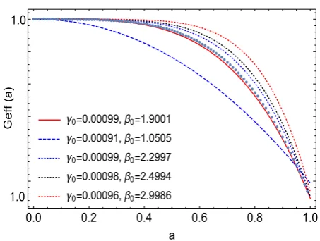
γ0=0.00099,β0=1.9001
γ0=0.00091,β0=1.0505
γ0=0.00099,β0=2.2997
γ0=0.00098,β0=2.4994
γ0=0.00096,β0=2.9986
0.0 0.2 0.4 0.6 0.8 1.0
1.0
a
Geff
(
a
)
1.0
Figure 1 The panel shows the plot ofGe f f function with curves defined by numerical values of (γ0,β0). The dotted blue line shows datapoints numerically calculated in the range a=[ami n, 1].
3.3 Numerical analysis on
G
e f f and effectiveNewtonian fields
We adopt for both cases of Γ±(a) the initial values of
γ0→0.001 andβ0→2. The numerical results of theGe f f
function is shown in the plot of Fig.(1). The related nu-merical datapoints were calculated within matter dom-inated era in the rangea=[ami n, 1] with the priors on
(γ0,β0) parameters. We observed that only the curves
con-structed in the rangeβ0=[1.9, 3] are well accommodated
to datapoints and obey the constraints onGe f f with low-values ofγ0≤0.001. On the other hand, higher values of γ0>0.001 and values ofβ0<1.9 andβ0>3 gradually
break down theGe f f constraints withGe f f(a=1)6=1 as
shown by the dashed blue line in Fig.(1).
From the numerical results of the analysis of Eq.(50) with a constraints on (η0,γ0,β0) allow us to solve
numeri-cally the density growth equation in Eq.(47). To facilitate referencing, we refer to our model asβ-model when nec-essary. Looking for a well behaved solutions for positive and negativeΓ, we adopt the values (γ0=0.001,β0=2.3)
for the first model, (γ0=0.0001,β0=2.5) for the second
one, and (γ0=0.0001,β0=3) for the third one. The
ini-tial conditions for Eq.(47) are set byδm(ami n)=ami nand
the related derivative with respect to expansion factor
δ0
m(ami n)=1. The results are presented in Fig.(2) with
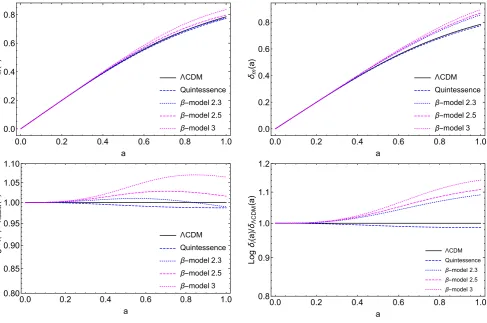
plots of numerical solutions forΛCDM (black line), GR quintessence (blue dashed line) and theβ-model fam-ily with the valuesβ0=2.3 (dotted blue line),β0=2.5
(dashed magenta line) andβ0=3 (dotted magenta line).
The top right and left panels show the results for the mat-ter growthδm(a) forΓ(+) andΓ(−). ForΓ(+)solution, it
shows a close compatibility at early times between the models and higher values of matter density growth of the modelβ0=3 (dotted magenta line) at late times as
com-pared toδmΛC D M(solid black line) and GR quintessence
(dashed blue line). ForΓ(−)solution in the top left panel, just as the previous case, it shows a close compatibility at early times between the models and more higher val-ues of matter density for the same set of valval-ues of the
β-model at late times as compared toδmΛC D Mandδm
for GR quintessence.
In the bottom panels, we can identify more clearly the differences of the rate of the growth by the ratioδi/δΛC D M
with the labelidenoting each model in comparison with
ΛCDM and GR quintessence. Just as in the previous case (top panels), at early times the models are indistinguish-able. On the other hand, at late times they are dramatically different. For bothΓ(±)solutions, they depart fromΛCDM pattern arounda=0.2. As compared withΛCDM, the maximum amplification of overdensities occur with the model forβ0=3 for bothΓ-solutions. It reaches around
6% forΓ(+)(bottom right panel) and 14% forΓ(−). In con-trast withΓ(−)solution, theΓ(+)forβ
0=2.3 presents a
mild damping of the growth of structures with a transi-tion arounda ∼0.9 getting closer to GR quintessence pattern. This is interesting fact since it might be taken into consideration into the dark matter debate on the ob-served underdensities on local Universe [75]. In summary,
β-model shows that the perturbations from extrinsic cur-vature provide the necessary gravitational power at least in sub-Hubble scale allowing room for an overall amplifi-cation up to 14% that may leave a trace in the CMB angu-lar power spectrum. Moreover, we analyse the percentage relative difference %diff(H−Hj) between theβ-models H,H1 andH2 for the valuesβ0=2.3, 2.5, 3, respectively.
Specifically, we show the difference withHΛC D Mfor both Γ-solutions as shown in Fig.(3). In those cases, we ob-tained at least a 10% difference for the lowest value of the modelβ0=2.3 and will be larger for higher values ofβ0.
This corroborates that theβ-model dynamics is rather different in comparison withΛCDM (or GR quintessence) due to the presence of theGe f f function.
In order to study the evolution of the Newtonian fields in Eqs.(49) and (51) they can be written in a more appro-priated form
Φk(k,a)= − 3 2k2Ω0H
2 0
Ge f f GN
a2ρmδm, . (52)
and also
Ψk(k,a)= − 3 2k2Ω0H
2
0Qe f fa2ρmδm, . (53)
ΛCDM Quintessence β-model 2.3 β-model 2.5 β-model 3
0.0 0.2 0.4 0.6 0.8 1.0
0.0 0.2 0.4 0.6 0.8
a
δm
(
a
)
ΛCDM Quintessence
β-model 2.3
β-model 2.5
β-model 3
0.0 0.2 0.4 0.6 0.8 1.0
0.80 0.85 0.90 0.95 1.00 1.05 1.10
a
Log
δi
(
a
)/
δΛ
CDM
(
a
)
ΛCDM Quintessence β-model 2.3 β-model 2.5 β-model 3
0.0 0.2 0.4 0.6 0.8 1.0
0.0 0.2 0.4 0.6 0.8
a
δm
(
a
)
ΛCDM Quintessence
β-model 2.3
β-model 2.5
β-model 3
0.0 0.2 0.4 0.6 0.8 1.0
0.8 0.9 1.0 1.1 1.2
a
Log
δi
(
a
)/
δΛ
CDM
(
a
)
Figure 2 Numerical solution of Matter density perturbations. The top panels show the comparisons ofΛCDM, GR quintessence andβ-model values forΓ(±)solutions. The bottom panels show the comparison with these models by the ratioδi/δmΛC D M.
%diff. H-H1
%diff. H-H2
%diff. H-HΛCDM
0.0 0.2 0.4 0.6 0.8 1.0
0 5 10 15
a
%
diff
.
Hi
-Hj
%diff. H-H1
%diff. H-H2
%diff. H-HΛCDM
0.0 0.2 0.4 0.6 0.8 1.0
0 2 4 6 8 10 12
a
%
diff
.
Hi
-Hj
Figure 3 The percentage relative difference%diff(H−Hj)between theβ-models forΓ(±)-solutions. The blue line shows a comparison withHΛC D M with a minimum of10%percentage difference.
Moreover, we use the conservation equation that of Eq.(15) with the initial valueρm(ami n)=ami n−3 and the
numerical results fromδmfor each study case ofβ0
LogΦ
LogΨ
LogΦ1
LogΨ1
LogΦ2
LogΨ2
-3.0 -2.5 -2.0 -1.5 -1.0 -0.5 0.0
10-12
10-1
109
1019
1029
Log(a)
Log
Φ
,
Log
Ψ
Figure 4 The decaying pattern (Logarithm scale) of the effec-tive Newtonian potentialsΦandΨfrom early to later times. The(Φ,Ψ)refers to theβ-model forβ0=2.3. The other mod-els are denoted by(Φ1,Ψ1)for β0=2.5and(Φ2,Ψ2)for β0=3.
ues in differentΓ-solutions. The initial field values are denoted byΦi ni=Φi ni(ami n) andΨi ni =Ψi ni(ami n) are
calculated atami n. The results of the behaviour of the
effective Newtonian potentialsΦandΨare presented in Fig.(4). It is interesting to note that at early times the po-tentials present higher values that rapidly (but smoothly) decay into lower values with a difference of 40 decimal places in logarithm scale, but are closer to 1 in linear scale calculated ata=a0=1. This reinforces the physical ro-bustness of our numerical analysis since the convergence of those potential are expected in Newtonian solar scale. This pattern happens to bothΓ-solutions. The observed “mild steps” in the curves are due to the change of signs of Eqs.(52) and (53) that induce mild fluctuations at that range but not capable of change the form of the curves into amplified oscillations. It may be possible that such amplifications may occur in a larger scale which is dif-ferent from the dark energy perturbations or modified gravity models such F(R) and variants, that are mostly neg-ligible at larger scales [76]. In each model, the presented curves ofΦandΨare indistinguishable.
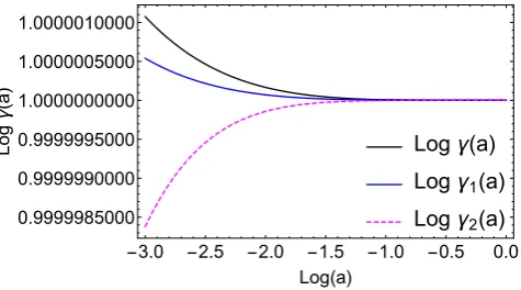
The anisotropy parameters in Eqs.(45) and (46) show better the difference between the fields indicating a phys-ical beyond GR. Theη(a) parameter measures the rela-tive change betweenΦandΨ, in a meanwhile theγ(a) indicates the absolute rate of change between them. In terms of these parameters, the variation of theΓ-solutions are practically indistinguishable and we present the re-sults in Fig.(5) and Fig.(6) valid for both solutions. In what concerns Fig.(5), higher values ofβ0lead to lower values
in early times. Interestingly, lower values ofβparameter
η1
η2
η3
-3.0 -2.5 -2.0 -1.5 -1.0 -0.5 0.0
10-16
10-13
10-10
10-7
Log(a)
Log
η
(
a
)
Figure 5 The decaying pattern (Logarithm scale) of the anisotropy parameterη(a)from early to later times. The bare
(η)refers to theβ-model forβ0=2.3. The other models are denoted by(η1)forβ0=2.5and(η2)forβ0=3.
Logγ(a)
Logγ1(a)
Logγ2(a)
-3.0 -2.5 -2.0 -1.5 -1.0 -0.5 0.0 0.9999985000
0.9999990000 0.9999995000 1.0000000000 1.0000005000 1.0000010000
Log(a)
Log
γ
(
a
)
Figure 6 The decaying pattern (Logarithm scale) of the anisotropy parameterγ(a)from early to later times. The bare
(γ)refers to theβ-model forβ0=2.3. The other models are denoted byγ1forβ0=2.5andγ2forβ0=3.
tends to provoke a higher difference between the poten-tials at early times. For instance, this is not expected in GR-ΛCDM in which the anisotropy parameterηis invari-antly zero andγis equal 1 for any period. Moreover, all the values converge at late times with mild fluctuations (mild spikes in Fig.(5)), which is corroborate by the anisotropic
γ(a) showing a mild difference in early times and a conver-gence for late times. It reinforces our priors that ofΦa0
Ψa0 =1. We stress that the analysis was taken just considering the fluctuations originated by the extrinsic curvature eventu-ally, as we can see in Eq.(44) and a more explicit difference is expected by adding the matter anisotropic stresses.
4 Summary
In this paper, we have analyzed the evolution of matter growth perturbations in the context of an embedding model in five dimensions to complement the concept of curvature in GR with the natural appearance of the ex-trinsic curvature. Our first results are related to the obtain-ment of the perturbed equations. Using the linear Nash-Green fluctuations, we have shown that only the gravita-tional tensor equation in Eq.(28) propagates cosmolog-ical perturbations, but the trace of Codazzi equation in Eq.(29) and Gupta equations in Eq.(30) remain confined to their background form. In the sub-horizon regime, we obtained a closed form of the effective Newtonian gravi-tational fieldΦand the effective Newtonian curvatureΨ modified by the presence of extrinsic. The related effec-tive Newtonian functionGe f f was calculated numerically
to constrain the parameters (γ0,β0) of the model since Ge f f constrainsGe f fca=0=1 andGe f fca=1=1 must be
in compliance of both Big Bang Nucleosynthesis and solar constraints. To guarantee aΛCDM background as an ini-tial reference for comparison, theη0parameter was fixed
to zero and was used to analyze the twoΓ-solutions that appear in the bending functionb(t) as shown in Eqs.(20) and (21). It is important to note that the obtainedGe f f
function does not depend on theΓ-solution and rein-forces its use to constrain the values for the parameters. Moreover, we obtained a tight range for allowed values forβ0=[1.9, 3] andγ0<0.001. The resulting numerical
analysis of growth equations leads to both scenarios of overdensities and a mild damping the growth of struc-tures (for a specific case withβ0=2.3) as compared with ΛCDM and GR quintessence. This results pinpoint an in-teresting direction to discussion of local voids within the dark matter halos debate. It was also shown the relative comparison of theβ-model with GR Lambda in which we obtain a range of 10% up to 14% of amplification of the matter fluctuations. This shows an indication of the extrinsic curvature dynamics may provide the necessary gravitational power to explain the growth of matter at large scale and the accelerated regime in the expansion of the universe and may imprint signatures on the CMB power spectrum.
In addition, we also have studied the evolution of the effective Newtonian potentialsΦandΨ. We have found a robust numerical compatibility between the initial pri-ors and related results that indicate a mild difference of those effective fields at early times and a convergence at late times to a lower values close to 1 that indicate a new physics different from GR. Those mild differences and fluctuations can be amplified with a consideration of the anisotropic stress from matter. Finally, we intend
to investigate further the implications of the obtained growth equation within a larger approach considering anisotropic matter stress and the level of sensibility the viscosity parameter within this framework. Also, the inte-grated Sachs-Wolfe effect to analyse an signature on CMB power spectrum will be a subject of future research.
5 Acknowledgements
The author thanks Federal University of Latin-American Integration for financial support from Edital PRPPG 110 (17/09/2018) and Fundação Araucária/PR for the Grant CP15/2017-P&D 67/2019.
Key words. Embedding; Gravity; Growth matter evolu-tion;Effective Newtonian constant
References
[1] Y. B. Zeldovich, JETP Lett. 6 316, 1967; Soviet Physics
Uspekhi,11 381, 1968.
[2] S. Weinberg, Rev.Mod.Phys., 61, 1, 1989.
[3] S. Weinberg,The Cosmological Constant Problems
(Talk given at Dark Matter 2000, February, 2000), ArXiv:astro-ph/0005265 (2000).
[4] I. Shapiro, Class. Quantum Grav., 25, 103001, 2008.
[5] C. P. Burgess,The Cosmological Constant Problem:
Why it’s hard to get Dark Energy from Micro-physics, ArXiv:1309.4133 [hep-th].
[6] P. J. Steinhardt,Cosmological Challenges for the 21st
Century, in Critical Problems in Physics, ed. V. L. Fitch, D. R. Marlow, M. A. E. Dementi, p. 123, 1997.
[7] H. E. S. Velten, R. F. vom Marttens, W. Zimdahl, Eur.
Phys. J. C74, 3160, 2014.
[8] S. Perlmutter, et al. Astrophys. J. ,517, 565, 1999.
[9] A. Riess, et al., Astron. J.116, 1009, 1998.
[10] V. Sahni, A. Starobinsky, Int. J. Mod. Phys.D15, 2105,
2006.
[11] W. J. Percival et al., Mon. Not. Roy. Astron. Soc.381,
1053, 2007.
[12] S. Alamet et al. (BOSS), Mon. Not. Roy. Astron. Soc.
470, 2617, 2017.
[13] M. Kowalskiet al. (Supernova Cosmology Project),
Astrophys. J.686, 749, 2008.
[14] A. H. Jaffeet al. (Boomerang), Phys. Rev. Lett.86, 3475,
2001.
[15] L. Izzo, M. Muccino, E. Zaninoni, L. Amati, M. D.
Valle, Astron. Astrophys.582, A115, 2015.
[16] G. Efstathiou and P. Lemos, Mon. Not. Roy.
As-tron.Soc.476, 151, 2017.
[17] S. W. Allen et al., Mon. Not. Roy. Astron.Soc.383, 879,
2008.
[18] E. Baxteret al., Mon. Not. Roy. Astron. Soc.461, 4099, 2016.
[19] R. Chávez, et al., Mon. Not. Roy. Astron. Soc.462,
2431, 2016.
[20] N. Aghanim et al., (Planck Collaboration), Planck
2018 results. VI. Cosmological Parameters, ArXiv:1807.06209.
[21] A. Klypin, A. Kravtsov, O. Valenzuela, F. Prada,
Astro-phys. J.522, 1, 89-92., 1999.
[22] B. Moore et al., Astrophys. J. Lett.524, 1, L19–L22,
1999.
[23] E. V. Karukes, P. Salucci, Mon. Not. R. Astron. Soc.465,
4703-4722, 2017.
[24] Navarro J.F., Frenk C.S., White S.D.M., Ap.J.490, 493,
1997.
[25] Salucci P., 2001, Mon. Not. R. Astron. Soc.344, L1.,
2001.
[26] Spekkens K., Giovanelli R., Haynes M.P., Astron. J.
129, 2119-2137, 2005.
[27] Ogiya G., Mori M., Astron. J.793, 1, 2012.
[28] de Blok, W.J.G., Adv. in Astron., Id.789293,14, 2010.
[29] A. Del Popolo, M. Le Delliou, Galaxies,5, 17, 2017.
[30] X. Fan, N. A. Bahcall and R. Cen., Astrophy. J. Lett.
490, 123, 1997.
[31] G. E. Addison, et al. Astrophys. J.853, 2, 119, 2018.
[32] R. A. Battye, T. Charnock, and A. Moss, Phys. Rev.D91,
10, 103508, 2015.
[33] S. Birrer et al., Mon. Not. Roy. Astron. Soc.484, 4726,
2019.
[34] I. G. Mccarthy et al., Mon. Not. Roy. Astron. Soc.476,
3, 2999, 2018.
[35] E. J. Copeland, M. Sami, S. Tsujikawa, Int. J.
Mod.Phys. D15, 1753, 2006.
[36] J. Frieman, M. Turner, D. Huterer, Ann. Rev.
As-tron.Astrophys.46, 385, 2008.
[37] L. Perivolaropoulos, AIP Conf. Proc.848, 698, 2006
[arXiv:astro-ph/0601014].
[38] L. Amendola, D. Polarski, S. Tsujikawa, Phys. Rev. Lett.
98, 131302, 2007.
[39] L. Amendola, R. Gannouji, D. Polarski, S. Tsujikawa,
Phys. Rev. D75, 083504, 2007.
[40] S. Nojiri, S. D. Odintsov, Phys. Rev. D74, 086005, 2006.
[41] S. Capozziello, S. Nojiri, S. D. Odintsov, A. Troisi, Phys.
Lett. B639, 135, 2006.
[42] S. D. Odintsov, V. K. Oikonomou, L. Sebastiani, Nucl.
Phys. B923, 608, 2017.
[43] S. Nesseris, G. Pantazis, L. Perivolaropoulos, Phys.
Rev. D96, 2, 023542, 2017.
[44] L. Kazantzidis, L.Perivolaropoulos, Phys. Rev. D97,
103503, 2018.
[45] R. Gannouji, L. Kazantzidis, L. Perivolaropoulos, D.
Polarski, Phys. Rev. D98, 104044, 2018.
[46] J. Pérez-Romero, S. Nesseris, Phys. Rev. D97, 023525,
2018.
[47] R. Arjona, W. Cardona, S. Nesseris, Phys. Rev.99,
043516, 2019.
[48] Randall L., Sundrum R., Phys. Rev. Lett.83, 3370,
1999.
[49] Randall L., Sundrum R., Phys. Rev. Lett.83, 4690,
1999.
[50] Dvali G., Gabadadze G., Porrati M., Phys. Lett.B485,
208-214, 2000.
[51] B. Carter, J.-P. Uzan, Nucl. Phys. B606, 45, 2001.
[52] J. Nash, Ann. Maths.63, 20, 1956.
[53] R. Greene, Memoirs Amer. Math. Soc.97, 1970.
[54] M. D. Maia, E. M. Monte, Phys. Lett. A297, 2, 9, 2002.
[55] M.D. Maia, N. Silva, M.C.B. Fernandes, JHEP0704,
047 (2007).
[56] M.D. Maia, E.M. Monte, J.M.F Maia, J.S. Alcaniz,
Class. Quant. Grav.22, 1623, 2005.
[57] M.D. Maia, A.J.S. Capistrano, J.S. Alcaniz, E.M. Monte,
Gen. Rel. Grav.10, 2685, 2011.
[58] A.J.S. Capistrano, Mon.Not.Roy.Astron.Soc.448, 1232,
2015.
[59] A.J.S. Capistrano, L.A. Cabral, Physica Scripta91,
105001, 2016.
[60] A. J. S. Capistrano, L. A. Cabral, Class. Quantum Grav.
33, 245006, 2016.
[61] A. J. S. Capistrano, Ann. Phys. (Berlin), 1700232, 2017.
[62] A.J. S. Capistrano, Phys. Rev. D100, 064049-1, 2019.
[63] T. Shiromizu, K. Maeda, M. Sasaki, Phys. Rev. D62,
024012, 2000.
[64] E. Anderson, R. Tavakol, Class.Quant.Grav.20, L267,
2003.
[65] V. Sahni, Y. Shtanov, JCAP(2003)0311, 014, 2003.
[66] S. Tsujikawa, M. Sami, R. Maartens, Phys. Rev. D70,
063525, 2004.
[67] Y. Gong, C. Duan, Mon.Not.Roy.Astron.Soc.352, 847,
2004.
[68] R. A. Battye, B. Carter, Phys. Lett. B509, 331, 2001.
[69] N. Arkani-Hamed, S. Dimopoulos, G. Dvali, Phys.
Lett. B429, 263, 1998.
[70] W. Pauli, M. Fierz. Proc.R.Soc.Lond. A173,211, 1939.
[71] S.N. Gupta, Phys. Rev.96, 6, 1954.
[72] C. J. Isham, A. Salam, J. Strathdee. Phys. Rev.3, 4,
1971.
[73] C. Fronsdal, Phys. Rev. D18, 3624, 1978.
[74] N. Rosen, Gen. Rev. Grav.4435, 1973.
[75] H. Böhringer, G. Chon, C. A. Collins, AA633, A19,
2020.
[76] J. C. Bueno Sanchez, L. Perivolaropoulos,
Phys.Rev.D81, 103505, 2010.