Exploring the Association between Network, Cognitive, Structural Social Capital and the Risk of Clinical Depression in Taiwan

University of South Carolina

Scholar Commons

Theses and Dissertations

8-9-2014

Applications of Electromagnetic Principles in the

Design and Development of Proximity Wireless

Sensors

Md Nazmul Alam

University of South Carolina - Columbia

Follow this and additional works at:https://scholarcommons.sc.edu/etd Part of theElectrical and Computer Engineering Commons

This Open Access Dissertation is brought to you by Scholar Commons. It has been accepted for inclusion in Theses and Dissertations by an authorized administrator of Scholar Commons. For more information, please [email protected].

Recommended Citation

A

E

P

D

D

P

W

S

by

Md Nazmul Alam Bachelor of Science

Bangladesh University of Engineering and Technology, 2006 Master of Science

Bangladesh University of Engineering and Technology, 2008

Submitted in Partial Fulfillment of the Requirements For the Degree of Doctor of Philosophy in

Electrical Engineering

College of Engineering and Computing University of South Carolina

2014 Accepted by:

Mohammod Ali, Major Professor Roger A. Dougal, Committee Member

Yong-June Shin, Committee Member Bin Zhang, Committee Member Jamil Khan, Committee Member

D

To my endless source of inspiration

My parents Nur-Jahan Alam & Md Shamsul Alam &

A

In the name of Allah, most gracious, most merciful. First and foremost, I would like to express my sincere gratitude towards Almighty Allah (swt) for nourishing me up to this level, guiding me through inevitably difficult times, and helping me to pursue my dream of completing my PhD.

Next, I want to thank my advisor, supervisor and mentor Dr. Mohammod Ali for expertly navigating me in the process of my PhD literature review, research, experiments, proposal and dissertation, without whom all things would have descended into chaos. His incredible ability to foresee future areas of difficulty in potential research, his persistent guidance, and his endless patience, resulted in my PhD dissertation and the finished dissertations of many other students as well. His thorough attention to my academic and personal requests has been highly appreciated. I thank him again for his tireless guidance and support all these years.

I would like to thank Dr. Roger Dougal, Dr. Yong-June Shin, Dr. Bin Zhang and Dr. Jamil Khan for serving on my proposal and PhD committees. Their suggestions, comments, and valuable time are highly appreciated. In particular, I would like to acknowledge the brilliant mind of Dr. Dougal for his expansive scientific expertise and invaluable feedback in the development of my research.

and especially bringing the joy of conducting research together. I am also very thankful to my colleagues in the Microwave Engineering Lab particularly Dr. Md Rashidul Islam and Nowrin Hasan Chamok. I would like to thank David Metts and other members of Department of Electrical Engineering for their helping attitude. Also, I would like to acknowledge my fellow friends in Columbia, South Carolina for their countless favors.

Last, but not least, my deepest gratitude is extended to my loving and loyal family, particularly my parents, my brothers and my extraordinary wife. My parents are my inside source of my inspiration. Their love, sacrifice, patience and teaching helped me to shape my moral and education background into what they are today. I am also deeply grateful to my wife; her unwavering commitment, continuous encouragement and moral support for all these days and many days to come.

Nazmul Alam

The University of South Carolina

A

Sensors and sensing system are playing dominant roles in monitoring the health of infrastructure, such as bridges, power lines, gas pipelines, rail roads etc. Sensing modalities employing Surface Acoustic Waves (SAW), Electromagnetic (EM) and optical have been investigated and reported. Sensors that utilize the perturbation of EM fields as function of the change in the physical structural or material phenomenon are of particular interest because of their inherent synergy with electronic system and diagnostic techniques, e.g. Time Domain Reflectometry (TDR), Joint-Time-Frequency-Domain-Reflectometry (JTFDR). The focus of this work is to study and develop new sensing and monitoring concepts that are based on EM principles.

T

C

DEDICATION ... iii

ACKNOWLEDGEMENTS ... iv

ABSTRACT ... vi

LIST OF TABLES ... xi

LIST OF FIGURES ... xii

LIST OF ABBREVIATIONS ... xvii

CHAPTER 1INTRODUCTION ...1

1.1 Motivation and Objectives ...1

1.2 Organization ...6

CHAPTER 2STATIC FIELD SENSING-INTERDIGITATED CAPACITOR FUNDAMENTALS ...8

2.1 Proximity Interdigitated Capacitor ...9

2.2 Analytical Solution of a Unit Interdigitated Cell ...10

CHAPTER 3STATIC FIELD SENSING-MOISTURE SENSING IN CONCRETE USING INTERDIGITATED SENSORS ...26

3.1 Sensor Geometry and Design Details ...27

3.2 Experimental Setup ...28

CHAPTER 4PROPAGATING WAVE SENSING-THE THEORY OF

SURFACE WAVE PROPAGATION ...37

4.1 Sommerfeld’s work ...38

4.2 Georg Goubau’s Work ...40

4.3 Elmore’s Work ...42

CHAPTER 5DESIGN AND APPLICATION OF SURFACE WAVE LAUNCHERS FOR NON-INTRUSIVE POWER LINE FAULT SENSING...45

5.1 Surface Wave Launchers and Their Transmission Properties...48

5.2 TDR Experiments Using CSW Launcher and VNA ...60

5.3 Circuit Experiment CSW Launchers ...63

5.4 Surface Wave Propagation Velocity Measurements in Unshielded XLPE Power Cables ...67

CHAPTER 6ANEW METHOD TO ESTIMATE THE AVERAGE DIELECTRIC CONSTANTS OF AGED POWER CABLES ...72

6.1 Mathematical Formulation to Estimate the Dielectric Constant of an Aged Cable ...75

6.2 Experimental Methodology ...82

6.3 Proposed Analysis and Results ...84

CHAPTER 7NON-INTRUSIVE ACCELERATED AGING EXPERIMENTS WITH SURFACE WAVE LAUNCHERS ...92

7.1 Experimental Setup for JTFDR with Wide Monopole Launchers ...93

7.3 Accelerated Aging Tests Results ...99

CHAPTER 8CONCLUSION AND FUTURE WORKS ...106

8.1 Contributions ...106

8.2 Future Works ...109

L

T

Table 2.1. Comparison between analytical solution and simulation results

from Ansys Maxwell 2D for different ...24

Table 5.1. Location of open circuit measured using VNA and CSW launcher ...62

Table 5.2. Location of open circuit measured using circuit and CSW launcher ...66

Table 5.3. Measured velocity of surface wave ...70

L

F

Figure 1.1. Some sensor use in civil infrastructure health monitoring. ...1 Figure 1.2. Sensors and sensing system (bridge image from google images);

a sensor node [4]. ...2 Figure 1.3. Rogowski coil sensor used for unshielded cable partial

discharge detection [19] ...5 Figure 1.4. Direct contact accelerated aging related fault detection

system using JTFDR ...5 Figure 1.5. Broadband antenna used for high frequency PD detection. ...6 Figure 2.1. Sensor system a system level diagram. ...8 Figure 2.2. (a) Conventional parallel plate capacitor (b) proximity

interdigitated capacitor [44]. ...10 Figure 2.3. The electric flux distribution for a unit interdigitated cell. ...11 Figure 2.4. Plot of the general inverse-cosine transformation

[43]. ...12 Figure 2.5. Fields between co-planar metal planes with a finite gap [43]. ...14 Figure 2.6. Field penetration depth, T mm versus electrode width w mm and the distance between the two electrodes, a mm...17 Figure 2.7. Field penetration depth, T mm versus electrode width w mm for a=0.05 mm,

0.1 mm, 0.2 mm, 0.5mm, 1mm and 5 mm. ...18 Figure 2.8. Electrode width, w mm versus field penetration depth T mm for,

a=0.05 mm, a=0.1 mm, a=0.2 mm, a=0.5 mm, a=1 mm and a=5 mm. ...19 Figure 2.9. versus the electrode width w and the distance between

Figure 2.10. versus the electrode width w and the distance between

two electrodes a. ...22 Figure 2.11. Plot of vector electric field in Ansys Maxwell 2D for W=10 mm

and a=10mm. ...22 Figure 3.1. The typical geometry of an interdigitated sensor. ...28 Figure 3.2. (a) Block diagram of sensor circuit and its (b) equivalent circuit. ...28 Figure 3.3. (a) Experimental setup to measure CDSfor concrete samples,

(b) placement of the sensor in the samples...31 Figure 3.4. Ansoft Maxwell 3D model of full circular sensor. ...32 Figure 3.5. Measured capacitance, CDS versus moisture content, MV for (a) the

meander sensor and (b) the full circular sensor. ...34 Figure 3.6. Comparison between the measured, analytical and simulated data

for the meander sensor. ...35 Figure 3.7. Comparison of measured and simulated capacitance for the full

circular sensor. ...35 Figure 4.1. Graphical representation of Sommerfeld’s wire/line with

finite conductivity ...39

Figure 4.2. Graphical representation of a Goubau wire/line ...41

Figure 4.3. Launching surface waves on a direct connected wire and receiving

them using horn antennas [41]. ...41

Figure 4.4. Glenn Elmore TM wave surface wave simulation model [65]. ...42

Figure 4.5. Elmore designed slotted horn antenna directly connected with a

bare aluminum power line cable reported in [65] ...43

Figure 4.6. Elmore measurement results of GAmax and transmission performance

Figure 5.2. Experimental setup of monopole surface wave launchers on

XLPE cable; cable length=2.14m. ...49

Figure 5.3. Measured S11 vs frequency of wire and wide monopole launchers in the presence and absence of a 2.14 m long XLPE unshielded power cable ...50

Figure 5.4. Measured transmission between monopoles with and without cable. ...51

Figure 5.5. Transmission response of the wide monopoles. ...52

Figure 5.6. HFSS model to simulate electric and magnetic fields. ...53

Figure 5.7. Comparison of simulated surface currents between the wire and wide monopoles in the presence of the XLPE cable. ...53

Figure 5.8. Computed H-field distribution along the cable (a) XZ plane and (b) YZ plane. ...54

Figure 5.9. Electric field (E) distribution in (a) XZ, and (b) YZ plane ...55

Figure 5.10. Proposed conformal surface wave launcher; (a) 3D view and bottom view, (b) installed on an unshielded power cable. The total ground plane dimension is 300 mm by 150 mm ...56

Figure 5.11. Transmission performance comparison for a pair of CSW launchers, wire monopole launchers and wide monopole launchers when placed on an XLPE cable of length 2.14 m. ...56

Figure 5.12. Transmission between a pair CSW launchers when placed against an XLPE power cable. ...59

Figure 5.13. Effect of ground height on the transmission between a pair of CSW launchers [79]. ...60

Figure 5.14. Effect of ground plane size on transmission for CSW launchers [79]. ...61

Figure 5.15. Results of TDR experiments using a single CSW launcher against four XLPE cables open circuited at the end [79]. ...62

Figure 5.16. The comparison of the generated pulse with a Gaussian pulse. ...64

of (a) 4.26 m (b) 9.45 m. Experimental results corresponding to the

setup shown in Fig. 5.18. ...66 Figure 5.19. Experimental setup to determine the surface wave propagation

velocity in an unshielded XLPE cable. ...69 Figure 5.20. Return signal observed in the oscilloscope for different XLPE

able. lengths and different pulse widths ...69 Figure 6.1. Experimental setup and definitions of terms. ...75 Figure 6.2. The experimental setup used in the accelerated aging

tests reported in [10]. ...82 Figure 6.3 (a). Total signal ( ) observed at oscilloscope.

6.3(b) Truncated signal corresponding to injected signal ( ) using rectangular time window at . 6.3(c) Truncated signal corresponding to

reflected signal from the end ( ) using rectangular time window at . ...85 Figure 6.4. Experimental phase plot with least square error fitted phase plot. ...86 Figure 6.5. Average dielectric constant, r1 determined using the proposed

method for XLPE insulated aged cable section. XLPE insulation

with aged section length = 1 m. ...87 Figure 6.6. Average dielectric constant, r1 determined using the proposed method

for EPR insulated cable section. EPR insulation with aged section = 1 m. ...87 Figure 6.7. The experimental setup used for artificial water intrusion in XLPE

cable. The wedged section is 2.5 cm long. ...88 Figure 6.8 (a). Total waveform ( ) of the cable under test before water

is introduced in the wedge (b) Total waveform ( ) of the cable under

test after water is introduced in the wedge...89 Figure 7.1. Non-intrusive accelerated aging test system functional diagram. ...94 Figure 7.2. Photograph of non-intrusive accelerated aging test. ...94 Figure 7.3. Direct contact method of JTFDR fault detection. Coaxial 10 m long

shielded XLPE power cable; 100 MHz center frequency of input waveform a) Input signal b) Output signal c) corresponding time-frequency

Figure 7.5. Non-Intrusive JTFDR waveforms for a 22.4 ft (6.83 m) unshielded XLPE insulated power cable along with 3.5ft coaxial instrumental cable using120 MHz JTFDR signal a) Input signal, b) reflected signal,

and c) corresponding time-frequency cross-correlated signal. ...98 Figure 7.6. Power spectra comparison between the input and

reflected signals of Fig. 7.5. ...98 Figure 7.7. a) The first reference input signal generated from

AWG ( ). b) Return

reflected signals for the unshielded cable at different aging periods ...100 Figure 7.8. Cross correlations at different aging periods for the first reference

signal ( ). ...101 Figure 7.9. a) The second reference input signal generated from

AWG ( ). b) Return

reflected signals for the unshielded cable at different aging periods. ...102 Figure 7.10. Cross correlations at different aging periods for second

L

A

BTS ... Bureau of Transportation Statistics

CSW ... Conformal Surface Wave

DOE ... Department of Energy

FDR ... Frequency Domain Reflectometry

GPR ... Ground Penetrating Radar

JTFDR ... Joint Time Frequency Domain Reflectometry

SAIDI ... System Average Interruption Duration Index

SAIFI... System Average Interruption Frequency Index

CHAPTER 1

INTRODUCTION

1.1 MOTIVATION AND OBJECTIVES

Sensors and sensing system are playing a dominant role in monitoring the health of infrastructure, such as bridges, pipelines, rail roads, and power lines. Wireless embedded sensors and sensing system present a unique opportunity because by embedding such sensors at critical locations of an infrastructure vital information can be obtained in real-time allowing rapid low cost monitoring and diagnostics. In recent years, researchers have studied various different kinds of sensors e.g. crack, moisture, strain, pH, accelerometer etc. for structural health monitoring [1-13]. Various structural health monitoring sensors are shown in Fig. 1.1.

Figure 1.1.Typical sensors used in civil infrastructure health monitoring.

Another critical infrastructure, where wireless sensors can play a vital role, is the electrical power grid. In many cases, power cables suffer premature failures due to various kinds of local stresses, including electrical, thermal, mechanical, chemical etc. Researchers are working on wireless sensors to monitor faults and continuous condition assessment of cables at different states, such as, open circuit, short circuit, partial discharge (PD), insulation damage, water and electrical tree formation in the insulation and high impedance fault [14-21].

Sensing modalities employing Surface Acoustic Waves (SAW), Electromagnetic (EM) and optical have been investigated and reported [22-23].

Sensors that utilize the perturbation of EM fields as function of the change in the physical structural or material phenomenon are of particular interest because of their inherent synergy with electronic system and diagnostic techniques, e.g. Time Domain Reflectometry (TDR), Joint-Time-Frequency-Domain-Reflectometry (JTFDR).

One particular application area that can benefit tremendously from an innovative EM sensor is an embeddable wireless moisture sensor for structural health monitoring.

Wireless sensor nodes

relative permittivity of 80 compared to dry concrete which is 4 at 100 kHz) it can be measured using a capacitive sensor. Increasing moisture will increase the sensor capacitance and hence the sensor output voltage. Moisture is unavoidable in structures yet they pose a serious problem resulting in crack in the concrete and corrosion in steel reinforcement. Since visual inspection is not possible embedded wireless moisture sensors will be greatly preferred. A simple two electrode capacitive sensor (typically used for soil moisture measurement in agricultural land) is too invasive and large [24]. Instead, a planar conformal sensor that is constructed of interdigitated electrodes will be a preferred choice because of its ease of integration with other electronics on a miniature circuit board. Various interdigitated sensors have been proposed for gas detection, resin curing, air humidity sensing and food moisture measurement [25-29]. However, the fundamental knowledge base that is required to design a miniature, conformal interdigitated sensor for embedded concrete moisture sensing is lacking. This includes an in-depth understanding of the design space that defines electric field penetration depth and its equivalent interelectrode capacitance as function of sensor geometrical parameters. 2D FEM simulation of such sensors to validate findings from static analytical solutions are also needed. Finally, sensors need to be designed, built and tested to validate that they meet those characteristics predicted by the analyses and modeling.

Thus, the first major focus of this dissertation is the development of the foundations

for static EM field sensing for moisture content measurement in materials.

on a power line to detect the emitted pulses from partial discharge [19]. One has to have some knowledge of where such PD will occur otherwise the coil will not be useful because of its location specific detection capacity. Moreover, because of its very low frequency operation high frequency emissions will not be detected. Researchers have used TDR, FDR and JTFDR for cable health monitoring including open circuit, short circuit, PD and insulation damage detection [30-37]. In a vast majority of the cases, the focus has been on conducted direct-contact measurements (see Fig. 1.4). Other researchers have used broadband antennas to detect PD pulses from cables and substations (see Fig. 1.5) [14, 38]. In this work, we consider EM antennas in conjunction with TDR and JTFDR methods to detect cable faults and insulation damage. While ordinarily an antenna is used in free space for communication applications the focus of this work is on using antennas as transducers that can inject a propagating surface wave at the conductor dielectric interface of a cable. Unlike earlier works of surface waves for communication and radar [39-42] our proposed approach considers non-intrusive subwavelength launchers and use the reflected wave signature to detect the location of the fault. Similarly as before, the fundamental know-how of propagating surface wave sensing for cable health monitoring needs to be developed. This includes investigating the feasibility of such an approach e.g. sensor size, type, signal frequency, bandwidth, transmission loss, range and the basic capacity to detect fault. This also includes the feasibility of non-intrusive cable insulation damage detection and estimating the changes in the average dielectric constant of the insulation material as function of cable aging.

Thus, the second major thrust of this dissertation is the development of the

Figure 1.4. Direct contact accelerated aging related fault detection system using JTFDR [36].

1.2 ORGANIZATION

In Chapter 2 the fundaments of static field sensing is formulated and then a unit interdigitated cell is characterized analytically using conformal mapping method. Analytical results of interelectrode capacitance are compared with results obtained from Ansys Maxwell 2D simulation for different sensor parameters.

In Chapter 3 to investigate the efficacy of the static electric field type sensing using interdigitated sensors the design, fabrication and experimental testing methods and the experimental results of a meander and a circular sensor are presented. Measurement results are compared with results obtained from Ansys Maxwell 3D static field simulator.

In Chapter 4 a concise review of surface wave propagation principles is presented followed by a brief literature review of surface wave launcher design and application.

In Chapter 5 the concept of surface wave launch and propagation as a non-contact sensing tool is demonstrated for open circuit fault detection in unshielded cables. Different laboratory prototypes are fabricated and measured to understand their frequency dependent return loss and transmission performance characteristics. Finally, a pulse generator circuit is designed and built to excite a nano-second TDR pulse using a Conformal Surface Wave (CSW) exciter to detect open circuit fault in cables.

In Chapter 6 a new mathematical method is presented to estimate the change in the average dielectric constant of aged power cables from JTFDR measurements from accelerated aging test based on the modified Arrhenius equation.

In Chapter 7 the application of surface wave sensing with JTFDR is demonstrated for accelerated thermal aging related insulation damage detection for unshielded XLPE cables.

CHAPTER 2

STATIC FIELD SENSING-INTERDIGITATED CAPACITOR FUNDAMENTALS

Measuring the moisture content in a material such as concrete using capacitive sensors is a very attractive solution. Interdigitated sensors are particularly interesting because of their planar conformal geometry, ease of fabrication and integration with circuit components. A system level diagram is shown in Fig. 2.1 which shows that measured output voltage being proportional to moisture in the Material Under Test (MUT) reflects the variation in the moisture. A microcontroller controls the measurement frequency and the measured output is wirelessly sent to a host station.

In order to design proximity interdigitated sensors, their fundamental characteristics such as field penetration depth and capacitance are studied using conformal mapping method. For comparison, 2-D FEM (Finite Element Method) simulations of a simple geometry are also performed.

Microcontroller Sensor on

MUT

A/D Converter

RF Transmitter

2.1 PROXIMITY INTERDIGITATED CAPACITOR

A regular capacitor consists of two electrical parallel plates separated by a dielectric material (solid, liquid or gas) (Fig. 2.2 (a)). The capacitance (C) is described as the relation between the charge distribution (Q) and the difference in the voltage (V); that is

(2.1)

The capacitance also depends on the geometrical shape of the conductor-dielectric arrangement and position. From Fig. 2.2 (a), the measured capacitance related to the dielectric constant of the material is

(2.2)

2.2 ANALYTICAL SOLUTION OF A UNIT INTERDIGITATED CELL

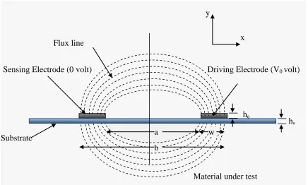
The geometry of the unit cell of an interdigitated sensor is shown in Fig. 2.3. The unit cell consists of a dielectric substrate with thickness hs and dielectric constant r1.

There are two conducting electrodes named the driving electrode and the sensing electrode each at a potential of V0 and 0 volt, respectively. The width of each electrode is

w and their separation distance is a. The conducting electrodes are each he thick. In

general this thickness is very small and thus he<<hs. The sensor unit cell is immersed in a

dielectric medium where it creates electric flux lines as illustrated in Fig. 2.3.

For simplicity of analysis, we did not consider the presence of a guard electrode. However, a guard electrode can be added and would be at ground potential. The guard electrode does not contribute in sensing but it provides immunity to the sensor from undesired Electromagnetic Interference (EMI). Also note that in the unit cell configuration a ground plane is not present.

The two-dimensional electric field distribution for the proposed scheme can be solved using conformal mapping techniques [43]. As the flux lines are elliptical and the equipotential lines are hyperbolic, the best way to attack this problem is to use inverse cosine transforms. Similar types of approaches were adopted in [43, 44]. As it is a solution of the two-dimensional electric field, the lengths of the electrodes are taken as

y

x Flux line

Material under test

Sensing Electrode (0 volt) Driving Electrode (V0 volt)

a w

Substrate

hs

he

b

infinitely long. The electric fluxes start at the driving electrode, penetrate the material under test (MUT) and then end at the sensing electrode. We made the following assumptions for this analysis,

1. The thickness of the MUT on either side of the sensor surface , must be greater than the field penetration depth T, corresponding to the maximum vertical displacement of field lines in the y direction, i.e., .

2. The substrate thickness is negligible compared to the height of the MUT i.e.,

, so that the flux distribution is not perturbed by the substrate material. 3. The electrode height is negligible compared to the height of the MUT i.e.,

. As a result, the direct fluxes between the two electrodes are also negligible.

Figure 2.4. Plot of the general inverse-cosine transformation

Referring to Fig. 2.4 suppose that we want to convert the rectangular plane plane to the inverse cosine plane plane.

Then, the general solution of the inverse-cosine transform is

_(2.3)

which means each assigned value of position vector in the plane has a specific corresponding value in the position in the plane. Therefore,

(2.4)

(2.5)

(2.6)

(2.7)

Then we can write,

(2.8) (2.9)

However, for this particular problem, a single pair of co-planar conducting plates of infinite length are surrounded by a homogeneous dielectric medium with permittivity of . The fixed potential of the right conducting plate (the driving electrode) is and the fixed potential of the left conducting plate(the sensing electrode) is 0. Therefore, the specific transformation will be

_(2.10)

(2.11)

(2.12)

The constant and are to be taken as real for this problem. Therefore,

(2.13)

Here, for our specific problem, the rectangular plane is the plane (see Fig. 2.3) and the transformed plane is plane (see Fig. 2.5).

Comparing Figs. 2.4 and 2.5, we want to be when to be unity, thus Then, when , we want and when , . Substituting these

w

Figure 2.5. Fields between co-planar metal planes with a finite gap [43].

, (2.14)

Hence the exact inverse-cosine transformation function with proper scale factor is

[ _{( )]} (2.15)

Where is the electrical potential function and is proportional to the electrical flux function.

From (2.15)

[ ] (2.16)

Therefore we can rewrite and in terms of and

[ ] [ ] (2.17)

[ ] [ ] (2.18)

From the above equations, we can easily separate and

( ) ( )

(2.19)

( ) ( )

(2.20)

( ) (2.21)

Maximum penetration would occur at the right most side of the electrode where and . From (2.18) we can write,

( ).

Or,

_{( )} (2.22)

So penetration depth,

[ _{( )]} (2.23)

Using hyperbolic trigonometry we can write,

√( )

(2.24)

According to Fig. 2.3, we can write

√( )

√( )

(2.25)

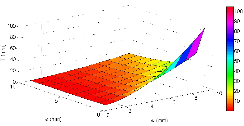
The variation of the field penetration depth T, with respect to from 1 mm to 10 mm and from 1 mm to 10 mm is plotted in Fig. 2.6. From this graph and also from (2.24), it is evident that the field penetration depth increases with the increase in

.Next figures, Fig 2.7 and Fig 2.8 also help us more to understand the relationship between T, a, and w.

In Fig. 2.7, we plot T versus w for the distance between the two electrodes varying from 0.05 mm to 5mm. The width of each electrode, w affects the penetration depth T more than the interelectrode separation a does. From the figure, for w=2 mm penetration depth increases from 2.5 to 3.7 mm while a increases from 1 mm to 5 mm. In contrast, the penetration depth doubles as w doubles.

Figure 2.7. Field penetration depth, T mm versus electrode width w mm for a=0.05 mm, 0.1 mm, 0.2 mm, 0.5mm, 1mm and 5 mm.

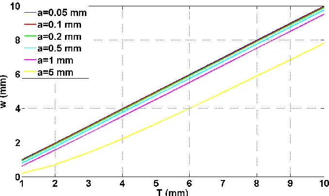
We can make similar observations from Fig. 2.8. These curves represent the design parameters for a certain penetration depth. For ‘a’ less than 0.5, the slope of the curves is nearly 1 and thus w=T. However, as ‘a’ increases ‘w’ diverges from the w=T relationship. For example, for a= 5mm and penetration depth 5 mm we need w=4 mm. For T less than 2 mm and a =5 mm, the w versus T curve is nonlinear. This can be explained from (2.27). When , (2.24) becomes which is a straight line

and again if , we can simply write .

We can also calculate the capacitance for this specific analytical model. The displacement vector is [23]

(2.26)

Figure 2.8. Electrode width w mm, versus field penetration depth, T mm for, a=0.05 mm, a=0.1 mm, a=0.2 mm, a=0.5 mm, a=1 mm and a=5 mm.

The total charge on the positive conductor can be approximated by integrating the electric displacement vector along the plane . However, along the plane on

the surface of the positive electrode( ), the potential equals to i.e.,

. Therefore, there is no derivative of electric flux( )

on this plane. Using Gausses

Law, we can derive the total electric charge present on the electrode

∮ ∫ | |

(2.27)

Solving (2.20) with respect to the boundary conditioni.e., and , we can write

(2.28)

Differentiating (2.18) with respect to y and using the boundary condition i.e., and

we can write,

( ) ( ) (2.29)

Therefore (2.27) becomes

Then, the total capacitance can easily be calculated using the potential difference between the electrodes which is for this specific case. Therefore,

[( ) √( ) ]

(2.31)

According to Fig. 2.3, , so we can rewrite the above equation

[ √( ) ] (2.32)

From (2.31) and (2.32), we can calculate the variation of the total capacitance with respect to the variation of and for a unit cell, if the other parameters remain constant. The variation of the total capacitance with respect to from 1 mm to 100 mm and is from 1 mm to 10 mm is plotted in Fig. 2.9 according to (2.31).

Figure 2.9 describes the surface plot of per unit length capacitance without considering the dielectric constant of the material (or considering only air) with respect to Figure 2.9. versus the electrode width w and the distance between two electrodes a.

electrode width ‘w’ and the distance between the two electrodes ‘a’. We can observe that capacitance decreases with increasing electrode separation ‘a’ and increases with increasing electrode width ‘w’. Fig. 2.10 further clarifies Fig. 2.9.

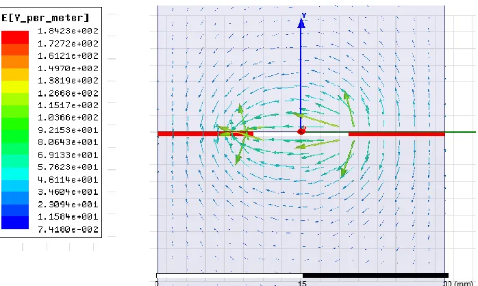
Figure 2.11. Plot of vector electric field in Ansys Maxwell 2D for W=10 mm and a=10mm.

Figure 2.10. versus the electrode width w and the distance between two electrodes a.

For comparison, we simulated a unit cell interdigitated capacitor using Ansys Maxwell 2D as shown in Fig. 2.11. The two red rectangular boxes represent the driving and the sensing electrodes. The driving electrode was set to and the sensing electrode was set to . The heights of the electrodes were set to 0.5mm. We assigned copper as their material property. The relative permittivity, of the material considered for the simulations was 2.2 (Duroid 5880). The two large light blue shaded boxes on the top and on the bottom represent the material under consideration. The heights of the boxes are 50 mm and the widths of the boxes are equal to the width of the unit cell. In Maxwell 2D, the solution method is electrostatic. The edges of the two boxes did not need to be explicitly defined because it remained as a natural surface. In Maxwell 2D, initially all the objects are surfaces that are predefined as natural boundaries, which means that the vector electric field is continuous across the surface. All outside edges of the metal boxes are defined as Neumann Boundaries, which means that the surface is continuous for tangential E field component and normal for D field component. The observed plot of the vector electric field is shown in Fig 2.11 for mm and

Table 2.1: Comparison between analytical solution and simulation results from Ansys Maxwell 2D for different .

(mm) (mm) Analytical equation (2.34) C/l (pF/m) Ansoft Maxwell 2D C/l (pF/m) Error

1 1 1 21.86 25.45

14%

2 1 2 28.43 32.3

12%

5 1 5 38.31 42.21

9%

10 1 10 46.34 50.13

7%

20 1 20 54.64 58.58

6%

2 2 1 21.85 25.51

14%

5 5 1 21.85 25.67

15%

10 10 1 21.85 25.34

14%

A comparison between the analytical (2.31) and simulation results is summarized in Table 2.1. As apparent, the percentage of error in the analytical simplified model results compared to the simulation results decreases from 14% to 6% as increases from 1 to 20. If both ‘w’ and ‘a’ are the same (for constant =1) such as 1, 2, 5 and 10 mm the

CHAPTER 3

STATIC FIELD SENSING-MOISTURE SENSING IN CONCRETE

USING INTERDIGITATED SENSORS

As mentioned, there has been a plethora of research activities on sensor design, development and system level integration to monitor the health of infrastructure, such as bridges, overpasses, airport runways etc. Measuring moisture inside concrete, particularly near the steel reinforcement is important because moisture is a precursor of corrosion [45].

interdigitated capacitor sensor should be preferred for concrete moisture content measurement because of its miniature size and conformal geometry. Justifiably, interdigitated sensors have been used in many applications in the past [49-52].

In this Chapter, the design and investigation of two interdigitated sensors are presented when used in concrete moisture content measurement.

3.1 SENSOR GEOMETRY AND DESIGN DETAILS

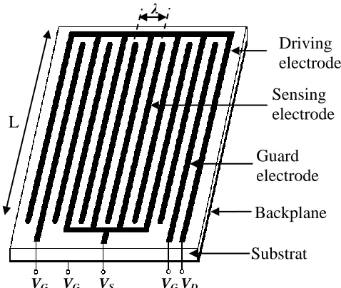
An interdigitated sensor is a coplanar structure consisting of multiple parallel fingers. The sensor can measure material dielectric constant by applying fringing electric fields into the material. The electrodes of the sensor must be in contact with the material under test. Fig. 3.1 shows the geometry of an interdigitated sensor [49]. Three types of electrodes are present, namely the driving electrode, the sensing electrode, and the guard electrode. A sinusoidal voltage VD is applied to the driving electrode and the output

voltage VS is measured from the sensing electrode. Guard electrodes and a conducting

backplane are used to shield the sensor from the influence of external fields [29]. Another important term is the field penetration depth, . A detailed analysis of is conducted and presented in Chapter 2 which showed that this parameter is a function of electrode width and spacing.

We used a simplified circuit model in Fig. 3(b) to calculate the capacitance between the driving and the sensing electrodes. The substrate has zero conductivity, so the current is due to the capacitive effect only. Also since the opamp is operating in the inverting mode, it is obvious that

(3.1)

(a) _{Virtual ground}

(b)

VG VG VS VGVD

λ

Sensing electrode Guard electrode Backplane Substrat e

Driving electrode

L

3.2 EXPERIMENTAL SETUP

To detect the percentage of moisture in concrete two interdigitated sensors were designed and fabricated. One was a meander sensor and the other was a circular sensor. Two sensor configurations were chosen to create different field penetration depths. The meander sensor is simpler and has smaller field penetration depth than the circular sensor. For the same field penetration depth the circular sensor covers a larger surface area than the meander sensor. The electrode width, height, gap and spatial wavelength of the meander sensor were 1.125 mm, 17 μm, 1.125 mm, and 4.5 mm, respectively. Thus the field penetration depth from Fig. 2.9 for the meander sensor is about 1.75 mm. For the circular sensor these dimensions were 1.5 mm, 17 m, 2 mm and 7 mm, respectively. Hence the field penetration depth for the circular sensor is > 2 mm. The meander sensor was fabricated on a 10 mil thick Duroid 5880 ( ) substrate and the circular sensor was fabricated on a 31 mil thick Duroid 5880 substrate. Referring to Fig. 3.1, the meander sensor had 7 driving electrodes, 4 sensing electrodes and 2 guard electrodes. The length of each electrode was 20 mm. For the circular sensor (see Fig. 3.5), the inner diameter of the innermost sensing electrode was 6 mm. The circular sensor had 12 driving electrodes, 10 sensing electrodes and 2 guard electrodes. Both sensors were coated with very thin perylene coating to avoid short circuit with the concrete, especially in the wet condition. A 1 kHz, 10V (peak) sinusoidal signal was chosen for VD. The

Concrete block samples were prepared using concrete mix. The age of the samples was more than one year at the time of the measurement. The dimensions of the samples were 15 cm 15 cm 2 cm and 15 cm 15 cm 4 cm.

The wet basis for the moisture content in a material is defined as

(3.6)

where mw is the mass of the specimen with water and md is the mass of the specimen in

dry condition. The moisture content of a material by volume Mv can be calculated as

(3.7)

where is the density of concrete in dry condition and is the density of water.

For measurement, the sensor was placed between two concrete samples. First, the sensor output voltage VF was measured for the samples in dry condition. Since VD was

known, the capacitance CDS was found using (3.1). After completion of the measurement

in dry condition the concrete samples were weighed in a scale to determine md. Then the

Wet samples were taken out from the water bucket. Since excess water present on the concrete surface had the potentials for erroneous results (high VF and high CDS) due to

the high permittivity of water the outer surfaces of the samples were wiped off using a dry cloth. The sensor was placed between the wet concrete samples. At regular periodic intervals, VF was recorded and the weight of the concrete samples mw was measured. For

each reading, CDS was found using (3.1) while the moisture content MV was found using

(3.6) and (3.7). Thus for each case a new MV and its corresponding CDS was found. Since

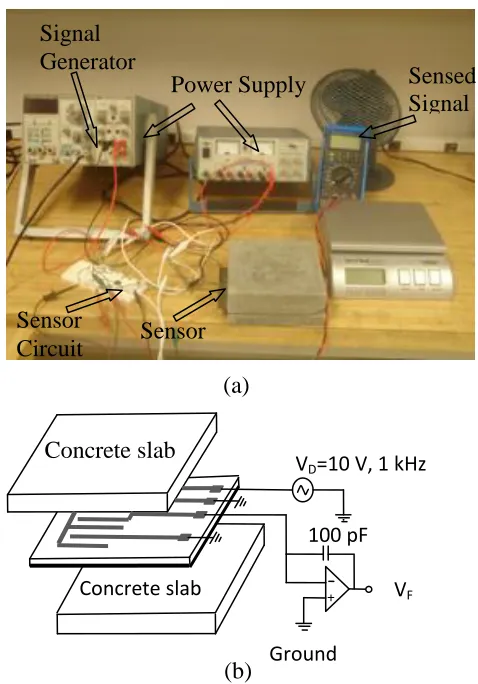
the evaporation rate depended on the environment, the ambient temperature and the air Sensed Signal Sensor Circuit Signal Generator Power Supply Sensor

VD=10 V, 1 kHz

Concrete slab

Concrete slab

Ground 100 pF

VF

Figure 3.3. (a) Experimental setup to measure CDS for concrete samples, (b)

placement of the sensor in the samples.

(a)

flow, an external fan was used to make the evaporation process faster.

3.3 RESULTS

3.3.1 EXPERIMENTAL RESULTS

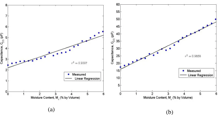
Measured CDS versus MV data for both the meander and the circular sensor are

shown in Fig. 3.6. A linear regression analysis was also performed on the measured data. From Fig. 3.6(a), in dry condition CDS =2.45 pF while for MV =5.968, CDS =5.548 pF.

The presence of water in the wet concrete clearly resulted in the increase in CDS(126.4%

increase). The sensitivity of the meander sensor is 0.519 pF/percent change in moisture content. Fig. 3.6(a) also shows that the coefficient of determination r2=0.9397 when

% 6 

v

M . Measured CDS versus MV results for the circular sensor are shown in Fig.

3.6(b). Since the field penetration depth of the circular sensor is larger than that of the meander sensor the resulting linear regression curve in Fig. 3.6(b) is steeper than the curve in Fig. 3.6(a). The coefficient of determination 0.9858. In dry condition

Figure 3.4. Ansoft Maxwell 3D model of full circular sensor. Concrete Sensing electrode

Driving electrode Guard electrode

CDS=17.385 pF while with MV =5.968, CDS =49.934 pF (187% increase). The sensitivity

of the circular sensor is 5.454 pF/percent change in moisture content.

3.3.2 COMPARISON BETWEEN EXPERIMENTAL AND SIMULATION

RESULTS

Ansoft Maxwell 3D was used to simulate the sensor responses for both the meander and the circular sensors. Fig. 3.5 is an example of the simulation model which was used for the full circular sensor. In the simulation, we were not able to account for the moisture content directly. In [53], experimental data of relative permittivity and conductivity versus frequency for four different levels of moisture content in concrete (from Fig. 2 of [53]) are available. These data are valid for the frequency range of 10 MHz to 1 GHz. We extended their curves down to 1 kHz using curve fitting in Matlab. Then we developed linear relations between the relativity permittivity and conductivity with percentage of moisture content using curve fitting. The resulting relative permittivity and conductivity values were used in our Maxwell simulations. The relative permittivity (r) and conductivity () of the concrete samples that were used in our simulation and

In Maxwell 3D the solution type was electrostatic. The driving electrodes were set to 10V and the other electrodes including the backplane were set to 0V. The default boundary condition, the Neumann homogeneous condition was used. The capacitances between the driving electrodes and the sensing electrodes were computed for the four different cases. Since the analytical equations (3.2) to (3.5) can only correctly describe the capacitance for the meander sensor, analytical results were obtained only for the meander sensor.

(a) _(b)

Figure 3.5. Measured capacitance, CDS versus moisture content, MV for (a) the

Comparison between the experimental, simulation and analytical data for the meander sensor is shown in Fig. 3.7. As seen, in general the agreement between all three is quite good. Some deviation is observed at higher moisture content levels. Fig. 3.8 illustrates the comparison between the experimental and simulation results for the circular sensor. Again, agreement is excellent for low moisture content. The measured Figure 3.7. Comparison of measured and simulated capacitance for the full circular sensor.

results are 10% to 20% higher than the simulated results for moisture contents larger than 4%.

CHAPTER 4

P

W

S

-

T

T

S

W

P

4.1 SOMMERFELD’S WORK

Sommerfeld [61] and his student Zenneck [40] first theoretically investigated the phenomenon of wave propagation over imperfect conductors known as surface waves. Sommerfeld theoretically investigated the propagation of non-radiating waves on a metal wire with finite conductivity and circular cross section. He also found that this non radiating mode is transverse magnetic and the wave solution came from the Maxwell equations. For example, if the wave is propagating in the +z direction, the field components are expressed as follows in the cylindrical coordinate system (see Fig. 4.1).

The radial component of the electric field is

(4.1)

The longitudinal component of the electric field is

_(4.2)

The magnetic field component in a plane transverse to the conductor is

(4.3)

Here, z indicates the distance along the cable and r indicates the distance from the wire center, is the propagation constant of the guided wave which is equal to . The free-space wave propagation constant inside and outside the wire is defined as

Outside the wire _√

where permeability, permittivity and conductivity and the subscript

indicates that the region is inside the wire. is the radial decay function defined by the following relations

_,

Where , where = wavelength of the surface wave. Inside the wire, the function is replaced by the Bessel function and outside the wire the function is replaced by the Hankel function of the first kind .

Suppose, is the radius of the finite conductive wire. Then and must be continuous at the surface which is the boundary condition of this problem. Therefore

Figure 4.1.Graphical representation of Sommerfeld’s wire/line with finite conductivity.

_(4.5)

From these above equations, other quantities such as attenuation, region of energy flow and other quantities can be calculated. For detailed analysis, please review [62]. Sommerfeld only considered the low frequency TM01 mode. Other higher order modes

may exist on a single wire transmission line, however in practical case, because of high attenuation they can be easily disregarded for long distance wave propagation [62].

4.2 GEORG GOUBAU’S WORK

Sommerfeld’s waves only exist for a conductor with finite conductivity. For Sommerfeld’s waves, if the conductivity is very high, the extension of the field goes to infinity. Georg Goubau suggested that coating a metal wire with dielectric or periodic corrugation will reduce the radial extension of the electric field by increasing the surface reactance. And for these cases, the conductivity does not have much effect on the extension of the radiated field [41, 63, 64]. Fig. 4.2 shows a graphical representation of a cable which supports TM waves according to Goubau’s principle. The field in the dielectric layer can be described by the Bessel function ( ) and the Neumann function ( ). Therefore, in (4.1)-(4.3) and can be replaced by

,

Using the boundary condition he derived that for the radius of the wire a and radius of the outher surface of the dielectric coating , the ratio becomes

( )

where ; √ . The subscript refers to the dielectric layer. The condition of wave propagation is that the phase velocity of the surface wave is slightly less than the velocity of the wave in free space. Consequently, Goubau also established that the dielectric layer should be thin compared to the wire radius and the combined wire plus dielectric radii should be smaller than the wavelength. The major contribution of Georg Goubau is that he experimentally demonstrated surface wave propagation [41, 63, 64].

Figure 4.3.Launching surface waves on a direct connected wire and receiving them using horn antennas [41].

H-field Horn antenna Horn antenna E-field

Coaxial line Coaxial line

He designed conical shaped horn antennas as surface wave launchers and connected those to the wire as shown Fig. 4.3. The transmit horn was energized using a signal source as shown in Fig. 4.3. The opening of the horns was 33 cm and the measurement was done at 1600 MHz on a 0.2 cm diameter wire (#12 wire) with an enamel thickness of 5x10-3 cm ( ). The length of the wire was 120 ft and the calculated total loss was 2 dB. His objective was to design a high frequency low loss single conductor transmission line. The details of his experiments and analysis are summarized in [41].

4.3 ELMORE’S WORK

Elmore proposed the application of surface waves for possible Power Line Communication (PLC) [42, 65]. His simulation studies consisted of surface wave launch and propagation along the length of a wire as illustrated in Fig. 4.4. Port 1 was connected between a large ground plane and the wire and a propagating wave was excited. Port 2

Figure 4.4. Glenn Elmore’s TM wave surface wave simulation model [8][65].

Ground plane Feed

100 mm

100 mm

0.04 mm conductor 4 mm conductor

400 mm

and the wire. Thus both transmission and reception was achieved by physically connecting the source and the receiver to the actual transmission medium, the wire.

His experimental work is shown in Fig. 4.5 which shows a large slotted horn antenna attached to an overhead power line. Surface wave propagation was achieved at 2 GHz. Fig 4.6 shows the measured S21 response of a pair of launchers that were 18 m

apart from each other and were placed on a #4 stranded copper power cable. The upper trace of Fig. 4.6 is the calculated GAmax presented by Elmore without considering the

attenuation due to port mismatch. At 1900 MHz, the insertion loss is 7 dB and at a second resonance at 500 MHz, the insertaion loss is about 27 dB. He also showed that his designed conical horn launcher was able to transmit 100 MHz of data bandwidth at 2 GHz with a C/N limit of 30 dB. He suggested possible application of his system might be for “Smart Grid” data communciation for end users along with real time power management and billing.

The Goubau or Elmore type surface wave launch and propagation is intrusive because it requires the RF or microwave signal source and the receiver to be physically connected to the wire or conductor that will support the wave propagation. In practical application, a non-intrusive method of signal injection is greatly preferred. Secondly, the wave launchers reported in the literature are large multi-wavelength travelling wave type launchers that are not suitable for application in the VHF-UHF frequency range which is the frequency range we are interested to test them out for power cable fault detection and monitoring using both TDR and JTFDR.

Figure 4.6.Elmore measurement results of GAmax and transmission performance S21

CHAPTER 5

DESIGN AND APPLICATION OF SURFACE WAVE

LAUNCHERSFOR NON-INTRUSIVE POWER LINE FAULT

SENSING

apparent that existing cable diagnostic techniques are complicated, bulky and heavy and do not allow real-time monitoring.

This Chapter introduces a concept of non-intrusive real-time power cable fault monitoring using wireless sensors (Fig. 5.1). The key components of the sensor are identified as energy harvester, waveforms and algorithms, circuits and components, and surface wave launcher. In [77] we have already reported a miniature energy harvester that can harvest power from a power cable non-intrusively. In terms of waveforms and algorithms, we propose to use TDR and in terms of circuits and components, we propose to use either commercial off the shelf elements or develop them in the lab. The key contribution of this work is the design, development and application of a pair of subwavelength sized broadband surface wave launchers, a TDR pulse generator circuit and the validation that when these are used in conjunction with the other building blocks identified in Fig. 5.1 one can detect power cable faults.

Medium voltage

cable

Low voltage cable

Figure 5.1. Examples of unshielded cables. Proposed non-intrusive wireless sensor

Crew working

Miniature snap-on

wireless sensors for overhead

unshielded power

Although studies of surface waves date back many years [40, 41, 63, 78] they have been recently revived to evaluate their potentials for data communication over power lines [65]. However, compared to the work described in [65] our research is fundamentally different since we propose to use surface waves as a sensing and diagnostic tool [15, 79], instead of its traditional application in communication. We propose to launch surface waves using distributed sensors (as shown in Fig. 5.1) and retrieve them using sensors to detect power cable faults. Once launched and during its travel if the wave experiences any fault that have a measurable impact on its propagation all or part of the wave is reflected. The reflected wave is then picked up by the wave launcher, and further processing then determines the location and extent of the damage.

5.1 SURFACE WAVE LAUNCHERS AND THEIR TRANSMISSION

PROPERTIES

5.1.1 WIRE AND WIDE MONOPOLE LAUNCHERS

As indicated, in this work the time domain reflectometry (TDR) technique is used along with a pair of surface wave launchers to detect power cable faults. An incident pulse travels down the length of a cable and then is reflected back from the fault location. By comparing the incident and reflected pulse waveforms we are able to detect and locate a fault. Typically in TDR, pulse durations are in the micro second range which requires that the surface wave launchers to be used should operate in the 50-500 MHz frequency range, have wide operating bandwidth and low loss. Since the non-intrusive sensors will be placed on power line cables the surface wave launchers also need to reside on the surface of the power cables. Previous surface wave launchers proposed by Goubau [41] and Elmore [65] are too large and are not of appropriate shape and weight to be accommodated on power cables. This led us to explore electrically small yet broadband non-travelling wave type antennas. These broadband antennas will work as surface wave launchers.

SMA connector was inserted and connected to the wire monopole. The ground plane was soldered to the ground connection of the SMA connector.

To investigate the feasibility of surface wave propagation using monopole launchers unshielded XLPE power cables were procured and used. The diameter of the sample XLPE cables was 16 mm including the insulation. The insulation thickness was 2 mm. The diameter of the wide monopole was slightly larger than 16 mm. A narrow slit was cut in the wide monopole for easy wrapping on the power cable.

Since the primary objective of this work is to launch relatively narrow time duration (hence broadband) pulses along the power cable and probe the return pulse two aspects are critical, e.g. launcher’s bandwidth (S11 and S21) and overall signal

transmission loss.

Thus to assess the bandwidth input S11 of the wire and wide monopoles were first

measured in air without any XLPE power cable to confirm launcher operation at around 250 MHz. Next the same experiments were repeated when a pair of launchers was placed at two ends of a 2.14 m long power cable (Fig. 5.2). These results are shown in Fig. 5.3 for both the wire and wide monopoles and both in the presence and absence of the power cable. It was observed that when the monopoles were in air the bandwidth was narrow. When the monopoles were placed on the XLPE cable insulation operation showed clear improvement in bandwidth. This is in line with the hypotheses that surface waves are propagating along the length of the cable resulting in a forward traveling wave along the length of the cable, hence less reflection and wider S11 bandwidth. Although S11

magnitude of -10 dB or lower is beneficial that may not be achievable with these resonant monopole type launchers. Thus unlike traditional communication antennas here we will use a more relaxed S11 limit to define bandwidth. Assuming S11<-5 dB the bandwidth of

either launcher in air without the XLPE cables is very narrow. A clear potential for wide Figure 5.3. Measured S11 vs frequency of wire and wide monopole launchers in the

bandwidth is 75-425 MHz when the wide monopole is brought close to the power cable.

In Fig. 5.4 we show the measured S21(dB) or transmission data between two launchers at

a distance of 2.14m. The two ports of a network analyzer were connected to two identical monopole launchers. Measurement with and without the XLPE cable between two wire monopoles are shown (black and red traces respectively). Clearly without the presence of the XLPE cable transmission is very weak. Transmission loss is between 45-70 dB within the frequency range of 50-200 MHz. In contrast, transmission loss is between 20-30 dB within the frequency range of 50-350 MHz when the XLPE cable is present. When the same experiment was repeated with two wide monopoles transmission improved significantly (Fig. 5.4) both in terms of signal strength and bandwidth. Similar results were obtained with other lengths of cables.

Figure 5.4. Measured transmission between monopoles with and without cable.

Fig. 5.5 shows the measured transmission data between two wide monopole antennas when separated by different lengths of XLPE cables. The cable length varies from 0.92 m to 2.14 m to 3.96 m. As apparent, there is a transmission dip near 60 MHz. For a frequency range of almost 80-300 MHz transmission is nearly flat with frequency. Clearly shorter lengths will allow better transmission and ensure that there are no significant transmission dips between the individual sensor nodes. For example, for 0.92 m cable length the worst case transmission dip is about -25 dB. But for 2.14 m and 3.96 m cables the worst case transmission dips are -40 and -50 dB respectively.

and developed and also sensor node density versus signal transmission loss has to be carefully evaluated.

Figure 5.7. Comparison of simulated surface currents between the wire and wide monopoles in the presence of the XLPE cable [79].

Since the cable does not have any other separate conductor nearby to allow a potential difference the propagating mode is a non-TEM (transverse electromagnetic) mode. To confirm this observation simulation models consisting of both the wire and wide monopoles were developed using HFSS [80]. In each model an 800 mm long XLPE cable was excited using a monopole at one end. Thus in one model the launcher was a wire monopole while in another model the launcher was a wide monopole.

A schematic of the HFSS model consisting of the wide monopole is shown in Fig. 5.6. Figure 5.8. Computed H-field distribution along the cable (a) XZ plane and (b) YZ plane [79].

(a)

monopoles are shown in Fig. 5.7. The top shows the current distribution due to the wire monopole while the bottom shows the current due to the wide monopole. It is clear that the wide monopole can create a more uniform current on the conductor of the XLPE cable which is distributed over the entire length of the cable. This corroborates our earlier observations that the wide monopole is low loss and has a wider transmission bandwidth than the wire monopole.

Similarly simulated magnetic field distributions are shown in Figs. 5.9 and 5.10 for a wide monopole surface wave launcher. Fig. 5.8 shows the magnetic fields in the Figure 5.9. Electric field (E) distribution in (a) XZ, and (b) YZ plane [79].

(a)

XZ and YZ planes. Here XZ is the plane normal to the axis of the cable and YZ is the plane parallel to the axis of the cable as shown in Fig. 5.6. We observe that the H field has no longitudinal component; all field vectors are in the transverse direction to the cable’s axis. Figs. 5.9(a) and (b) show the electric fields in the XZ and YZ planes.

Figure 5.11. Transmission performance comparison for a pair of CSW launchers, wire monopole launchers and wide monopole launchers when placed on an XLPE cable of length 2.14 m.

Figure 5.10. Proposed conformal surface wave launcher; (a) 3D view and bottom view, (b) installed on an unshielded power cable. The total ground plane dimension is 300 mm by 150 mm

(a)

Electric fields have both transverse and longitudinal components. Thus clearly the two monopole system on the cable supports TM mode surface wave propagation.

5.1.2 CONFORMAL SURFACE WAVE LAUNCHERS

The wire and wide monopole launchers designed and studied before are not conformal due to the metallic ground plane that is orthogonal to the power cable. This led us to consider developing a surface wave launcher which is conformal and can be placed on a plane parallel to the plane of a power cable. The primary idea was to use a ground plane that is not in the shape and size that was used for the wire and wide monopoles. Instead the idea of a folded ground plane was considered. Thus the new launcher named conformal surface wave (CSW) launcher consists of a wide monopole and a ground plane that is parallel to the power cable. In order to create more surface area for the ground plane the ground plane was folded multiple times. Between each fold a thin insulating layer was placed. This structure resembles an Inverted L Antenna (ILA). An ILA is a monopole antenna with lower radiation resistance, narrower bandwidth, and modified radiation pattern compared to a wire monopole antenna [81]. Without additional matching an ILA is not an efficient far field antenna [82]. However far field performance is not our concern as the surface wave launcher is not a far field device. The folded ground plane occupies much less space but has about the same area as that of the unfolded ground plane.

narrower than the wide monopole. The transmission loss of the CSW monopole is also higher than the wide monopole. Both of these clearly indicate the limitations of miniaturization. Although the folded ground plane seems to offer performance it is a worse alternative than the wide monopole with the orthogonal ground plane. Nevertheless, because of its small size and conformal nature it may be more amenable for actual use on a power cable. Undoubtedly best bandwidth and signal transmission can be obtained if travelling wave type surface wave launchers can be developed and used. They will be multiple wavelengths in size, heavy and may not be necessary for power system application. Thus future applications will dictate what type of bandwidths will be needed and what should be the density of the sensor nodes and then based on these data one may proceed to design and develop optimum size surface wave launchers.

Transmission performance was also measured by varying the separation between the CSW launchers when placed against an XLPE cable. The prototype CSW launcher had monopole length of 300 mm. The folded ground plane size was 300 mm by 150 mm. The ground plane was at a height of 5 mm from the monopole. Fig. 5.12 shows the transmission performance for separations of 0.92 m, 2.14 m and 3.96 m.

The transmission between a pair of CSW launchers when placed against a 2.14 m XLPE cable was also measured by varying the ground plane height. The ground plane height was varied as 1 mm, 5 mm, 10 mm and 20 mm. For ground plane heights of 5 mm, 10 mm and 20 mm there were no significant effect on the transmission (see Fig. 5.13). But transmission degraded significantly as the ground plane height was reduced to 1 mm. Experiments were also performed as function of ground plane sizes, e.g. 300 mm x 225 mm, 300 mm x 150 mm, 150 mm x 150 mm and 150 mm x 75 mm. Fig. 5.15 shows these results. For the 300 mm x 225 mm ground, the ¬20 dB transmission band extends from 85-265 MHz. For the 300 mm x 150 mm ground, there are two transmission bands, 90-200 MHz and 365-395 MHz. For the 150 mm x 150 mm ground there are also two transmission bands 90 to 115 MHz and 360-550 MHz. For The transmission bands for the 150 mm x 75 mm ground are from 105 to 130 MHz and from 380 to 525 MHz. Thus it is clear that increasing the ground plane size will increase the transmission bandwidth of the CSW launcher.