DIRECTION OF ARRIVAL AND STATE OF
POLARIZATION ESTIMATION USING RADIAL BASIS FUNCTION NEURAL NETWORK (RBFNN)
S. H. Zainud-Deen, H. A. Malhat, K. H. Awadalla and E. S. El-Hadad
Faculty of Electronic Engineering Menoufia University
Egypt
Abstract—A Neural Network architecture is applied to the problem
of Direction of Arrival (DOA) and state of polarization estimation using a uniform circular cross and tri-crossed-dipoles antenna array. A three layer Radial Basis Function Network (RBFN) is trained with input output pairs. The network is then capable of estimating DOA not included in the training set through generalization and the corresponding state of polarization. This approach reduces the extensive computations required by conventional super resolution algorithms such as MUSIC and is easier to implement in real-time applications. The results suggest that the performance of the RBFNN method approaches the exact values. In real time, fast convergence rates of neural networks will allow the array to track mobile sources.
1. INTRODUCTION
Super-resolution algorithms have been successfully applied to the problem of Direction of Arrival (DOA) estimation to locate radiating sources with additive noise, uncorrelated and correlated signals. MUSIC [1] and [2] and ESPRIT [3] and [4] are some of the popular conventional methods of DOA estimation. They have the advantage of high resolution for signals with small angular separation (few degrees to few tenths of a degree). However, one of the main disadvantages of these algorithms is that they require extensive computation and are difficult to implement in real-time.
presented in [5–10]. The main advantages of the neural network methods are that they outperform conventional linear algebra based methods in both speed and accuracy. Since neural methods avoid the cumbersome eigen-decomposition process, they are found to be far quicker than conventional methods. Apart from being computationally efficient, neural methods have been observed to be more immune to noise and are found to yield better performance in the presence of correlated arrivals. However, a drawback of the neural schemes is the selection of the network size which is usually done by trial and error.
In this paper, the application of neural networks to handle the computational problem of the DOA estimation step is approached as a mapping problem which is modeled using a Radial Basis Function Network or (RBFN) that can be trained with input output pairs [11–13]. The network is then capable of estimating or predicting outputs not included in the learning phase through generalization. Moreover, one of the main advantages of neural networks is that they can be implemented in analog circuits with time constants in the order of nanoseconds and consequently they have fast convergence rates. Thus DOA estimation problem is viewed as a function approximation problem, and the RBFNN is trained to perform the mapping from the space of the sensor array output to the space of DOAs. It exploits the universal function approximation capability of RBFNN to estimate the DOA and the state of polarization and a successful classification of closely separated sources (3 degrees) has been reported.
2. DOA ESTIMATION USING REAL ELEMENT ARRAYS
The signal processing algorithms proposed for DOA estimation provides accurate estimates, even in moderate signal to noise (SNR) conditions, but generally ignore the electromagnetic behavior of the receiving antenna. The receiver is assumed to be an ideal, equispaced, linear array of isotropic point sources and does not reradiate the incident signals. In practice, this ideal situation cannot be met. The elements mutual coupling distorts the linear phase front of the incoming signal, significantly degrading performance. Thus any practical implementation of DOA estimation requires compensation for mutual coupling. The compensation of mutual coupling using effective techniques has been reported in [14–16].
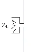
By using impedance load at each element port as shown in Fig. 1, the measured voltage at the port of the nth receiver antenna is given by
ZL
Figure 1. The compensation for mutual coupling in real array
elements using load at terminal pointZL= 50 Ω.
i.e., the measured voltage at a port of the array is directly proportional to the coefficient of the basis function corresponding to that port.
3. RBFNN MODEL FOR DOA PROBLEM
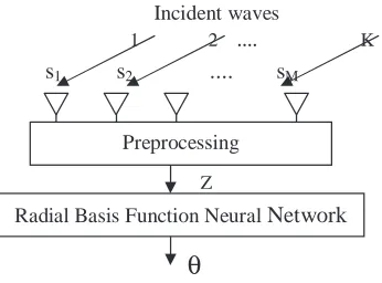
The DOA problem is approached as a mapping which can be modeled using a suitable neural network (NN) trained with input output pairs. The network capable of estimating or predicting outputs not included in the learning through generalization. The advantages of NNs are that it can be implemented in real time. The adaptive antenna array can be linear array or circular array with isotropic or real elements. Neural networks based direction finding algorithms have been proposed for single and multiple source direction finding [17]. It has been shown that the neural networks have the capability to track sources in real time. It has been suggested that a radial basis function neural network (RBFNN) could be used to track the locations of mobile users [18].
Preprocessing
Radial Basis Function Neural Network
θ Z Incident waves
1 2 .... K
s1 s2 .... sM
Figure 2. Proposed architecture of DOA estimate using neural
network.
4. DATA PREPROCESSING
It considers a linear array composed ofM elements (point sources), and letK(K≤M) be the number of plane waves, centered at frequencyωo
impinging on the array from directions{θ1 θ2 . . . θK}. It performs the mappingG: RK →CM from the space of DOA, {θ= [θ1, θ2, . . . , θK]}
to the space of sensor output {s = [s1, s2, . . . , sM]}, where sM is the
source output at elementm, namely
sm = K
k=1
akej(m(ωo/c)dsinθk+αk (2)
where ak represents the complex amplitude of the kth signal, αk the
initial phase, andωo is the center frequency. Based on the information
theoretic criteria for model selection [19], one can estimate the number of signalsK a priori.
The RBFNN is used to perform the inverse mapping F: CM → RK. The network is to be trained by N patterns generated by using
Eq. (2) so that it can associate the output vectorss(1), s(2), . . . , s(N) with the corresponding DOA vectors θ(1), θ(2), . . . , θ(N). Input vectors s are mapped through the hidden layer then each output node computes a weighted sum of the hidden layer outputs. We can write for a set data {(s(i), θ(i)), i= 1,2, . . . , N}. The output of the neural is given by
θk(j) = N
i=1
wkifh(s(j)−s(i)2) (3)
weight of the network. Using the Gaussian function for hidden nodes
fh, we can rewrite Eq. (3) as
θk(j) = N
i=1
wkie−s(j)−s(i)2/σ2g (4)
the parameterσg controls the influence of each basis function.
The main advantage of using an RBFNN over other approaches is that it does not require training the network with all possible combinations of input vectors. For the network to generalize it is sufficient to perform the training with vectors that span the expected range of input data.
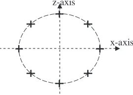
x-axis z-axis
Figure 3. 16-elements uniform circular array (crossdipole) geometry inx-z plane.
5. NUMERICAL RESULTS
5.1. The Uniform Circular Array Geometry
coordinate system is located in the center of the array. The angular position of thenth element of the array is given by [20]
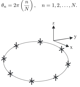
θn= 2π
n
N
, n= 1,2, . . . , N. (5)
y
x
z
Figure 4. 24-elements uniform circular array (tri-crossed-dipoles).
The narrowband plane wave with wavelengthλ(and correspond-ing wave numberk= 2π/λ) arrives at the antenna from elevation angle
θ and azimuthal angle ϕ. The using of cross-dipoles and Tri-crossed-dipoles as a UCA elements are useful in obtaining different states of polarization ant different planes of incidence [21].
5.2. Example (1) Cross-dipole Uniform Circular Array
A circular array of M = 16 cross-dipoles each of length λ/2, are terminated in loadsZL= 50 ohm is used. Therefore, the dimension of
the input layer of the neural network was set to 16 nodes (magnitude of the input vector Vn(n)). The array receives signal with different
0 50 100 150 200 0
50 100 150 200
N
Ao
A
0 50 100 150 200
0 50 100 150 200
N
Ao
A
desired RBFNN desired
RBFNN
0 50 100 150 200
0 50 100 150 200
N
AO
A
0 50 100 150 200
0 50 100 150 200
N
Ao
A
desired RBFNN desired
RBFNN
(a) (b)
(c) (d)
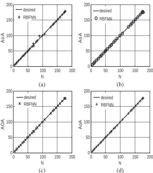
Figure 5. DOA estimates versus number of samplesN for cross-dipole array. Incident Source (1)ϕis varied from 0◦to 180◦andθ= 90◦when (a) linear-θ polarized, (b) linear-ϕ polarized, (c) right-hand circular polarized, (d) left-hand circular polarized.
0 50 100 150 200
0 50 100 150 200
N
Ao
A
0 50 100 150 200
0 50 100 150 200
N
Ao
A
desired RBFNN desired
RBFNN
0 50 100 150 200 0 50 100 150 200 N Ao A
0 50 100 150 200
0 50 100 150 200 N Ao A desired RBFNN desired RBFNN (c) (d)
Figure 6. DOA estimates versus number of samplesN for cross-dipole array. 8-Uncorrelated sources used with (∆ϕ= 3◦). Source (1) ϕ is varied from 0◦ to 180◦ and θ= 90◦.
-100 -50 0 50 100
-100 -50 0 50 100 N AO A
-100 -50 0 50 100
-100 -50 0 50 100 N AO A desired RBFNN desired RBFNN
-100 -50 0 50 100
-100 -50 0 50 100 N AO A
-100 -50 0 50 100
-100 -50 0 50 100 N AO A desired RBFNN desired RBFNN (a) (b) (c) (d)
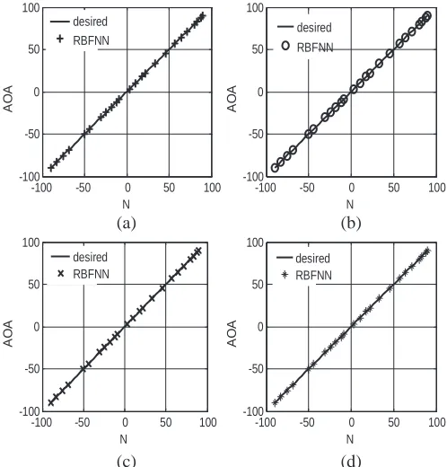
Figure 7. DOA estimates versus number of samples N for tripole
5.3. Example (2) Tri-crossed-dipoles Uniform Circular Array
A circular array of M = 24 tri-crossed-dipoles array each of length
λ/2, are terminated in loads ZL= 50 ohm is used. The array receives
signal with different state of polarization. The array is exposed by incident plane wave source in different planes and the performance of the RBFNN is shown in the figures. Figs. 7, 8, and 9 shows the RBFNN performance with DOAs were assumed to be uniformly distributed from −90 to 90 in both the training and testing phases in the planesϕ= 0, 45◦, and 90◦ respectively. Fig. 10 shows the RBFNN performance with DOAs assumed to be uniformly distributed from 0◦ to 180◦ in both the training and testing phases in the x-y plane. Similarly Fig. 11 and Fig. 12 shows the network performance when the array receives eight uncorrelated signals with different angular separations (∆θ = 5◦ and ∆ϕ = 3◦) at different planes respectively. The results show that the network successfully produced actual outputs very close to the desired DOA.
-100 -50 0 50 100
-100 -50 0 50 100
N
AO
A
-100 -50 0 50 100
-100 -50 0 50 100
N
AO
A
desired RBFNN desired
RBFNN
-100 -50 0 50 100
-100 -50 0 50 100
N
AO
A
-100 -50 0 50 100
-100 -50 0 50 100
N
AO
A
desired RBFNN desired
RBFNN
(a) (b)
(c) (d)
Figure 8. DOA estimates versus number of samples N for tripole
-100 -50 0 50 100 -100
-50 0 50 100
N
AO
A
-100 -50 0 50 100
-100 -50 0 50 100
N
AO
A
desired RBFNN desired
RBFNN
-100 -50 0 50 100
-100 -50 0 50 100
N
AO
A
-100 -50 0 50 100
-100 -50 0 50 100
N
AO
A
desired RBFNN desired
RBFNN
(a) (b)
(c) (d)
Figure 9. DOA estimates versus number of samples N for tripole
array. Incident Source (1)θ is varied from −90◦ to 90◦ and ϕ= 90◦.
0 50 100 150 200
0 50 100 150 200
N
AO
A
0 50 100 150 200
0 50 100 150 200
N
AO
A
desired RBFNN desired
RBFNN
0 50 100 150 200 0 50 100 150 200 N AO A
0 50 100 150 200
0 50 100 150 200 N AO A desired RBFNN desired RBFNN (c) (d)
Figure 10. DOA estimates versus number of samples N for tripole
array. Incident Source (1)ϕ is varied from 0◦ to 180◦ and θ= 90◦.
-100 -50 0 50 100
-100 -50 0 50 100 N AO A
-100 -50 0 50 100
-100 -50 0 50 100 N AO A desired RBFNN desired RBFNN
-100 -50 0 50 100
-100 -50 0 50 100 N AO A
-100 -50 0 50 100
-100 -50 0 50 100 N AO A desired RBFNN desired RBFNN (a) (b) (c) (d)
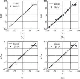
Figure 11. DOA estimates versus number of samples N for tripole
0 50 100 150 200 0
50 100 150 200
N
AO
A
0 50 100 150 200
0 50 100 150 200
N
AO
A
desired RBFNN
desired RBFNN
0 50 100 150 200
0 50 100 150 200
N
AO
A
0 50 100 150 200
0 50 100 150 200
N
AO
A
desired RBFNN
desired RBFNN
(a) (b)
(c) (d)
Figure 12. DOA estimates versus number of samples N for tripole
array. 8-Uncorrelated sources used with (∆ϕ= 3◦). Source (1) ϕ is varied from 0◦ to 180◦ and θ= 90◦.
6. CONCLUSION
The neural network is used to estimate the direction of arrival with different arrays such as circular arrays with real elements of cross-dipoles and tri-crossed-cross-dipoles elements, where the RBFNN is trained by input-output pairs to estimate the DOA with different separated angles and tested with samples are not included in the learning phase. Good agreement between the results using the RBFNN model, and the exact values.
REFERENCES
2. Kautz, G. M. and M. D. Zoltowski, “Performance of MUSIC employing conjugate symmetric beamformers,” IEEE Trans. Signal Processing, Vol. 43, 737–748, 1995.
3. Rao, B. D. and K. V. S. Hari, “Performance analysis of ESPRIT and TAM in determining the direction of arrival of plane waves in noise,” IEEE Trans. Acoust., Speech, Signal Processing, Vol. 36, 1990–1995, 1989.
4. Vigneshwaran, S., N. Sundarajan, and P. Saratchandran, “Directional of arrival (DOA) estimation under array sensor faliures using minimal resources allocation neural network,”IEEE Trans. Antennas Propagat., Vol. 55, No. 2, 334–343, February 2007.
5. Haykin, S., Neural Networks: A Comprehensive Foundation, Prentice Hall, New York, 1999.
6. Chang, P. R., W. H. Yang, and K. K. Chan, “A neural network approach to MVDR beamforming problem,”IEEE Trans. Antennas Propagat., Vol. 40, 313–322, Mar. 1992.
7. Christodoulou, C. and M. Georgiopoulos, Applications of
Neural Networks in Electromagnetics, Artech House, Norwood,
Massachusetts, 2001.
8. Mohamed, M. A., E. A. Soliman, and M. A. El-Gamal, “Optimiza-tion and characteriza“Optimiza-tion of electromagnetically coupled patch an-tennas using RBF neural networks,”J. of Electromagn. Waves and Appl., Vol. 20, No. 8, 1101–1114, 2006.
9. Guney, K., C. Yildiz, S. Kaya, and M. Turkmen, “Artificial neural networks for calculating the characteristics impedance of air-suspended trapezoidal and rectangular-shaped microstrip lines,” J. of Electromagn. Waves andAppl., Vol. 20, No. 9, 1161–1174, 2006.
10. Ayestar´an, R. G., F. Las-Heras, and J. A. Martinez, “Non uniform-antenna array synthesis using neural networks,” J. of Electromagn. Waves andAppl., Vol. 21, No. 8, 1001–1011, 2007. 11. Southall, H. L., J. A. Simmers, and T. H. O’Donnell, “Direction
finding in phased arrays with a neural network beamformer,” IEEE Trans. Antennas Propagat., Vol. 43, 1369–1375, Dec. 1995. 12. El Zooghby, A. H., C. G. Christodoulou, and M. Georgiopoulos, “Performance of radial basis function networks for direction of arrival estimation with antenna arrays,” IEEE Trans. Antennas Propagat., Vol. 45, 1611–1617, Nov. 1997.
basis function neural networks,” IEEE International Symposium on Antennas andProp. Digest, 203–206, 1998.
14. Gupta, I. J. and A. A. Ksienski, “Effect of mutual coupling on the performance of adaptive array,”IEEE Trans. Antennas Propagat., Vol. 31, 785–791, Sept. 1983.
15. Adve, R. S. and T. K. Sarkar, “Compensation for the effects of mutual coupling on direct data domain algorithms,”IEEE Trans. Antennas Propagat., Vol. 48, 86–94, Jan. 2000.
16. Lau, C. K. E. and R. S. Adve, “Minimum-norm mutual coupling compensation with applications in direction of arrival estimation,” IEEE Trans. Antennas Propagat., Vol. 52, No. 8, 2034–2040, Aug. 2004.
17. Canning, F. X., “Direct solution of the EFIE with half the computation,” IEEE Trans. Antennas Propagat., Vol. 39, 118– 119, Jan. 1991.
18. Virga, K. L. and Y. Rahmat-Samii, “Efficient wide-band evaluation of mobile communications antennas using [Z] or [Y] matrix interpolation with the method of moments,”IEEE Trans. Antennas Propagat., Vol. 47, 65–76, Jan. 1999.
19. Wax, M. and T. Kailath, “Detection of signals by information the-oretic criteria,” IEEE Trans. Acoust., Speech, Signal Processing, Vol. 33, 387–392, 1985.
20. Balanis, C. A., Antenna Theory: Analysis andDesign, Third Edition, Wiley, New York, 2005.