A Volume-Surface Composite Scattering Model for Nonlinear Ocean Surface with Breaking Waves and Foam Layers Under High Wind Conditions

A Volume-Surface Composite Scattering Model for Nonlinear Ocean

Surface with Breaking Waves and Foam Layers under High

Wind Conditions

Xiaoxiao Zhang1, *, Xiang Su2, and Zhensen Wu3

Abstract—Electromagnetic scattering from the sea surface is of great significance in ocean remote sensing especially under high wind conditions. A novel volume-surface composite scattering model of nonlinear rough sea surfaces with breaking waves and foam layers under high wind conditions is presented in this study. Based on the semi-deterministic facet scattering model (SDFSM), using a ray tracing method combined with impedance equivalent edge currents (RT-IEEC) and vector radiative transfer theory (VRT), the backscattering characteristics of the sea surface with breaking waves and foam layers are investigated. The crest- and static-foam coverage was introduced to determine the breaking point and foam coverage distribution. The dependence of the backscattering coefficient of the sea surface with and without breaking waves and foam layers on the incident angle, wind speed, and the polarization are discussed in detail. The results of numerical simulations are analyzed and compared with the measured data from the relevant references which verifies the validity of our volume-surface composite scattering model. The synthetic aperture radar (SAR) image simulations of the surface with and without the breaking waves and foam layers are compared, and the combined effects of the breaking waves and whitecaps are analyzed.

1. INTRODUCTION

The study of the electromagnetic scattering mechanism from the sea surface is of great significance in remote sensing systems and target recognition with complex background [1]. The research on the electromagnetic scattering model of the sea surface can not only help to estimate and optimize the target recognition algorithm, but also be used to supplement experimental data [2–4]. The high-resolution radar characteristics of the sea surface under high wind conditions at low grazing angles (LGA) have been a point of discussions and in-depth analysis in recent years [5–8]. Under high wind conditions, the wave energy increases due to sea-air interactions, and wave breaking occurs. Wave breaking not only limits the height of surface waves by transferring momentum flux from waves to currents, but also generates marine aerosols and entrains bubbles that modify the emissivity and scattering properties of the ocean surface [9]. The extent of the illuminated area of the sea surface is very large at LGA, thus the irradiated region contains not only longer wavelengths of gravity waves and shorter wavelengths of tension waves, but also breaking waves, whitecaps, and other fine structures. All these waves and breaking events are reflected in the spatial variation of clutter returns. The classical composite scattering models tend to yield satisfactory results at high and medium grazing angles. However, the scattering mechanisms are much more complex at LGA, and the observed results deviate from the traditional scattering model.

In these situations, strong, target-like returns from the sea, which are also called sea spikes, are always present in the case of horizontal polarization due to the non-resonant backscatter caused by

Received 20 June 2019, Accepted 9 August 2019, Scheduled 27 August 2019

* Corresponding author: Xiaoxiao Zhang (zhangxiao [email protected]).

breaking waves and whitecap. However, they are sometimes absent in the case of vertical polarization due to the dominance of resonant scatter with this polarization. The spike amplitudes for the HH returns have much higher contrasts against their backgrounds with the largest peaks exceeding the corresponding VV returns [10]. The difference between HH and VV polarizations cannot be fully described in the framework of the resonant approach.

In the past decades, a considerable number of theoretical models have been constructed to elucidate and understand the scattering processes involved in such problems. To sum up, several physical scattering mechanisms have been proposed to explain the sea spike echoes. These include specular backscatter from the steep front of the breaking wave, backscatter enhancement due to multipath effects from the wave itself and from the foot of the breaking wave, Brewster damping of VV [11–13], diffraction from wedge features [14, 15], and reflection from foam layers [16, 17]. However, the attempts at theoretical modeling mentioned above, including numerical models and analytical models, have been carried out to describe the sea spike at LGA based on only some of these scattering components. Models proposed so far to calculate the scattering characteristics from the sea surface are unable to fully describe all the marine components contributions. Recently, several new models have been proposed for the scattering from the sea surface with breaking waves, but with no attention paid to the wedge diffraction or foam layer effects [18, 19]. In order to understand the issue more comprehensively, we need to solve two problems regarding the backscatter from surface with breaking waves and foam layers. (1) A method to determine the breaking point and the foam coverage distribution must be developed, and (2) an appropriate model for the breaking waves covered with foam layers on the upwind side must be selected, which can analytically obtain the dominant effects including specular scattering of the breaking front, multipath backscatter, wedge diffraction, and foam scattering, efficiently.

Waves break is a complex dynamic process. The LONGTANKE model [20] and other models [21, 22] based on hydrodynamic theory can describe the breaking wave shapes more precisely and are often used for calculating the scattering of individual breaking waves numerically. However, for large marine areas, a wedge-like model can analytically obtain the dominant effects efficiently. Thus, such a wedge-like model is still thought to be reasonable by many authors [14, 18, 23].

According to the shape and brightness of whitecap images obtained from airborne platform high resolution radar, Bondur and Sharkov [24] found that the whitecap formations can be divided into two types: (1) fresh dense foam patches from breaking waves (crests-foam) (2) low-reflectance residual foam layers (static-foam). The authors of [25, 26] suggested a model of the relationship between crest- and static-foam coverage, thickness, and wind speed that gives us the basis of the breaking point and foam coverage distribution.

In this study, a novel volume-surface composite scattering model is proposed to investigate the electromagnetic scattering properties of the sea surface with breaking waves and foam layers. This study is organized in the following order. Section 2 deals with the generation of a nonlinear Creamer II sea surface. The crest- and static-foam coverage and the thickness of the foam layers varied with the wind speed are presented in this section. The composite model of the nonlinear sea surface with breaking waves and foam layers is then established via a slope criterion. In Section 3, the volume-surface composite scattering model for electrically large sea volume-surface with breaking waves and foam layers is introduced. In Section 4, the statistical behavior of the returns and the relationship of the spatial properties with both the incident angles and wind speeds for different polarizations from the sea surface with breaking waves and foam layers are presented. The validity of the model has also been proven against the measured data. SAR images of the nonlinear sea surface with and without consideration being paid to the breaking waves and foam layers are simulated and compared. Finally, in Section 5, a summarizing discussion is presented, and some further improvements of the model are addressed. These improvements will be investigated in greater depth in a future study.

2. GEOMETRIC MODEL OF THE SEA SURFACE WITH BREAKING WAVES AND FOAM

scatterometric data [27] is introduced by the following formula to determine the slope distribution of the breaking waves.

P(zx,0) = 10−2.84+0.097u10−1.33zx (1)

where u10 is the wind speed at 10 m height above the mean level of sea surface, and zx is the slope of

x-direction for breaking waves.

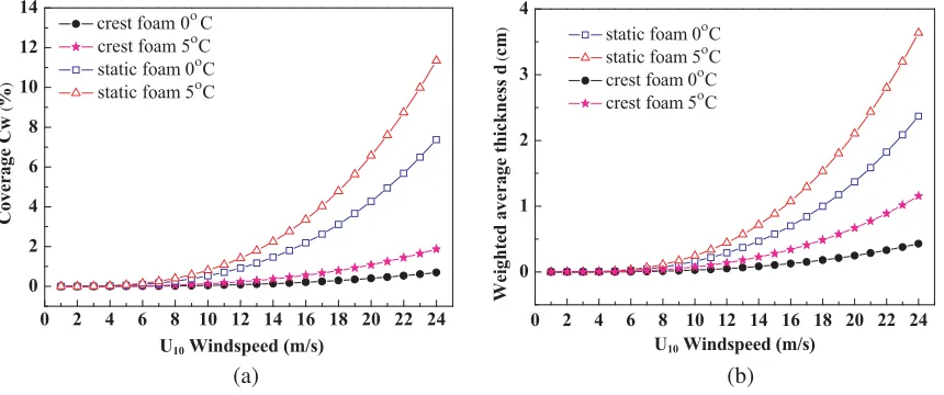
Based on [25], the whitecap formations are divided into crests of dynamic foam and patchy structures of static foam, respectively. Fig. 1(a) shows that the coverage varied with the wind speed both for the crest- and static-foam for two different values of temperature difference between air and water ΔT(◦)C (ΔT =Tsea−Tair). The dependence of the weighted average thickness of the foam on the

wind speed is shown in Fig. 1(b). We observe that both the foam coverage and thickness increase with the wind speed. If ΔT increases from 0◦C to 5◦C, the fractional coverage due to crest- and static-foam increases by about a factor of 2.7 and 1.5, respectively.

0 2 4 6 8 10 12 14 16 18 20 22 24 0

2 4 6 8 10 12 14

crest foam 0οC crest foam 5οC static foam 0ο_C static foam 5οC

U10 Windspeed (m/s)

Coverage Cw

(

%

)

0 2 4 6 8 10 12 14 16 18 20 22 24 0

1 2 3 4

Weighted average thickness d

(

cm

)

U10 Windspeed (m/s) static foam 0οC

static foam 5οC crest foam 0οC crest foam 5οC

(a) (b)

Figure 1. The crest-foam and static-foam coverage and thickness of foam layers varied with wind speeds. (a) Coverage; (b) Thickness.

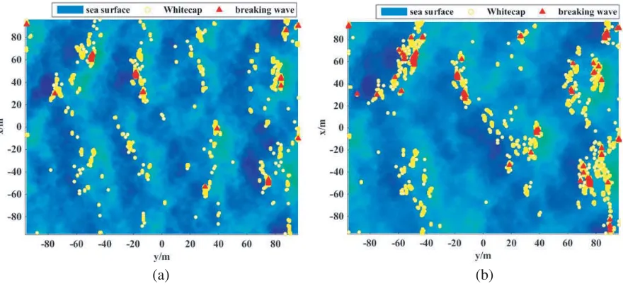
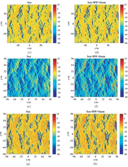
Figure 2 shows the breaking waves and foam distributions of a sea surface at different wind speeds. The area of the surface is 192 m×192 m, and the discrete sampling points along thex andy directions areM =N = 256. The coverage of breaking waves and foams increases significantly with the increase in wind speeds, which is in accordance with Fig. 1.

The key parameters describing the sea foam are the air void fractionfa, bubble sizers, and number

of bubbles per unit volumeN that is related to the volume fractionfv byN = 3fv/(4πrs3). For sea foam,

we assume seawater as the environment and air bubbles as inclusions, thus fv =fa and the dielectric

constant of sea foamεf is determined by [28]

εf =εe+ 3fvεe εi−εe

εi+ 2εe−fv(εi−εe)

(2)

whereεe and εi are the permittivity of the environment and the inclusions, respectively. In this study,

we choose fa = 0.98, rs = 2 mm. Once these parameters are fixed, the extinction coefficient κe and

volume scattering coefficientκs can be determined by

κs=

8 3πN k

4

errs6 εr−1

εr+ 2 2

κe=κa+ 2ke(1−fv) +fvkeεr

_εr3_{+ 2}2

(3)

whereεr =εi/ε0 =εr−jεr is the relative dielectric constant, andke andke are the real and imaginary

(a) (b)

Figure 2. The breaking waves and foam distribution of the sea surface at different wind speeds. (a)

u10= 13 m/s; (b)u10= 20 m/s.

3. SCATTERING MODEL OF SEA SURFACE WITH BREAKING WAVES AND FOAM

Scattering from the illuminated ocean surface for LGA incidence is very complex and intractable. The structures of the illuminated ocean surface range from the tiniest capillary ripples to large scale fully developed swells and must include the effects of breaking waves and foam. In Section 2, we have discussed how a slope criterion can be applied to geometric model of the sea surface with breaking waves and foam layers. This section will present the volume-surface scattering model of the sea surface. We will concentrate on the contribution of the wedge-like breaking waves and foam layers to the clutter radar cross sections (RCS).

3.1. Scattering from Rough Sea Surface

Based on the semi-definite scattering model, scattering from local wind-derived ripples is approximated by Bragg (or resonant) scattering, and the tilting of the ripples by longer waves changes the scattered power [29]. The total scattering coefficients of each facet can be expressed by combining the long and short waves contributions that can be obtained by the Kirchhoff Approximation and the Tilted Small Perturbation Model (TSPM) [30].

σijtotal(ki,ks) =σijT SP M(ki,ks) +σijKA(ki,ks) (4)

Here,

σpqKA(ki,ks) =πk2q2|Upq|2P

zxtan, zytan q4z

σpqT SP M(ki,ks) =πk4|ε−1|2|Fpq|2Sζ(ql)

(5)

wherekis the wave number of the incident wave;q =|q|=|k(ˆks−ˆki)|; Upqis the polarmetric coefficient

(pq indicates H- or V-pol);P(zxtan, zytan) is the Cox-Munk PDF [31];zxtan, zytan is the slope of the tangent

plane at the specular point; and qz is the z-component of q. Further, ε is the permittivity of the

surface;Fpq is the polarmetric coefficient; Sζ(ql) is the spatial power spectrum and can be expressed as

Sζ(ql) = ψsea(k)/ql; ψsea(k) is the Elfouhaily capillary spectrum; andql is the projection of vector q

A

ˆ

x

ˆ

n

ˆ i k ˆ i k 1 r 2

r

r

4

r

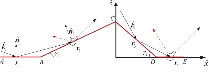
Figure 3. Muti-scattering from the wedge-like breaking wave.

3.2. Wedge-Like Breaking Wave Scattering

The wedge-like breaking wave (shown in Fig. 3) is constructed from rectangular plates of dimensions BC for the downwind side and DE for the upwind side (AB and BC designate the area around the wedge). Taking the downwind observation as an example, there are six scattering path combinations from the radar to wedge-like breaking waves, each with different induced currents: (i) single scattering from plate AB; (ii) double scattering from plate AB to plate BC; (iii) single scattering from plate BC; (iv) single scattering from plate CD; (v) double scattering from plate CD to plate DE; (vi) single scattering from plate DE. We still treat plates AB and DE as rough surfaces, and the single scattering from rough plates AB and DE is obtained from the semi-definite scattering model. The scattering from the crest BCD and the double scattering is obtained using both geometrical and physical optics. Taking the double scattering (path ii) from plate AB to plate BC for instance, the incident field at point r1 on plate AB for HH polarization is

Ei_1HH =

ˆ ei·ˆh

ˆ hE0exp

−jkˆk1i·r1

(6)

The incident field at pointr2 on plate BC after the reflection from plate AB and path attenuation is

Ei_2HH =

ˆ ei·ˆh

ˆ

hR1HHexp

−jkˆk1i·r1

·E0exp

−jkˆk1r·(r2−r1) (7)

Thus, the reflection field isEr_2HH =R2HHEi_2HH, and the total field is Etotal= (1 +R2HH)Ei_2HH. The

induced magnetic current at point r2 can be obtained by (τˆ=−nˆ2׈h) M2HH(r2) = −nˆ2×Etotal

= ˆτ

(1+R2HH)R1HH

ˆ ei·ˆh

×E0exp

−jkˆk1i·r1

exp

−jkˆk1r·(r2−r1) (8)

The induced electronic current can be obtained by the same way:

J2HH(r2) = nˆ2×Htotal

= −1

η

ˆ n2·ˆki2

(1−R2HH)R1HH

ˆei·ˆh

ˆ

h×E0exp

−jkkˆ1i·r1

exp

−jkˆk1r·(r2−r1) (9)

For VV polarization, the induced current can be expressed as

J2V V(r2) =nˆ2×Htotal =

1

η

ˆ n2׈h

(1 +R2V V)R1V V (ˆei·ˆv)

×E0exp

−jkˆk1i·r1

exp

−jkkˆ1r·(r2−r1)

M2V V(r2) =−nˆ2×Etotal =−hˆ

ˆ n2·ˆki2

(ˆei·vˆ) (1−R2V V)R1V V

×E0exp

−jkˆk1i·r1

exp

−jkkˆ1r·(r2−r1)

We can get the total induced current

J2(r2) = 1

η

ˆ n2׈h

(ˆei·vˆ) (1 +R2V V)R1V V −

ˆ n2·kˆi2

(1−R2HH)

ˆei·hˆ

ˆ hR1HH

×E0exp

−jkˆk1i·r1

exp

−jkkˆ1r·(r2−r1)

M2(r2) =−

(nˆ2×hˆ)(1 +R2HH)

ˆ ei·hˆ

R1HH +

ˆ n2·ˆki2

(ˆei·ˆv)hˆ(1−R2V V)R1V V

×E0exp

−jkˆk1i·r1

exp

−jkkˆ1r·(r2−r1)

(11)

The far scattering field due to the induced current of the plate BC is

Es(r) = −jωμ0

4πr exp(−jkr)

×

BC

J2(r2)−

J2(r2)·ˆk2s ˆk2s+

ε0

μ0

M2(r2)×kˆ2s exp

jkr2·ˆk2s

dr2 (12)

When Eq. (11) is substituted into Eq. (12), we obtain

Es(r) = jωμ0

4πrE0exp(−jkr)×

BC

exp

jkr2·ˆk2s−jkˆk1i·r1−jkˆk1r·(r2−r1) dr2

1

η

ˆ

k2s׈k2s×

ˆ n2׈h

(ˆei·vˆ)(1 +R2V V)R1V V

−1

ηˆk2s׈k2s×

ˆ n2·ˆki2

(1−R2HH)

ˆ ei·ˆh

ˆ hR1HH

+ ε0 μ0 ˆ n2׈h

(1 +R2HH)

ˆ ei·ˆh

R1HH׈k2s

+ ε0 μ0 ˆ n2·kˆi2

(ˆei·vˆ)hˆ(1−R2V V)R1V V ׈k2s

(13)

The internal form in Eq. (13) can be written as

I =

BC

E0exp

jkr2·ˆk2s−jkˆk1i·r1−jkˆk1r·(r2−r1) dr2

= jE0exp(−jT2) [exp(−jT1xC)−exp(−jT1xB)] ΔY /T1 (14) whereT1= (k1rx−k2sx)+(k1rz−k2sz) tanγ1, andT2 = (k1rz−k2sz)(h−tanγ1xC). The single scattering

from plate BC and CD can be obtained easily, and the double scattering from plate CD to plate DE can be analytically expressed in the same manner.

3.3. Wedge Diffraction Effect

The perturbation method proposed by Lyalinov et al. [32] is used in this study to build the spectral functions for computing the diffraction coefficientD for the scattering by the impedance wedge at skew incidence. For almost normal incidence, the spectral function can be expressed as follows:

Se,h(α) = Ψe,h(α)σφ0(α) ∞

m=0

ξe,h(α) cosmβ (15)

where Ψe,h(α) is the traditional Maliuzhinets’ function, andφ0 is the incident angle measured from the wedge face.

σφ₀(α) =

1 nsin φ0 n sinα

n −cos φ0

n

where n is defined by the exterior wedge face angle nπ. The leading term of the perturbation series

ξe,h(α) in Eq. (15) can be expressed directly by the Maliuzhinets’ work

ξe,h0 (α) =Ue,hi /Ψe,h(nπ/2−φ0) (17) whereUe,hi is the incident electromagnetic field amplitude.

The first order term can be obtained by the perturbation method

ξh1(α) =−Uei

jsin(α/n) 4nπΨe(nπ/2−φ0) ×

⎧ ⎪ ⎪ ⎪ ⎪ ⎪ ⎪ ⎪ ⎨ ⎪ ⎪ ⎪ ⎪ ⎪ ⎪ ⎪ ⎩ j∞

−j∞

cost

cos(t/n)

Ψe(nπ/2 +t)−Ψe(nπ/2−t)

(sint+ sinθ0

h)Ψh(nπ/2 +t)

×[σ1(t, α)−σ1(t, nπ/2−φ0)]dt

+

j∞

−j∞

cost

cos(t/n)

Ψe(nπ/2 +t)−Ψe(−nπ/2−t)

(sint+ sinθhn)Ψh(−nπ/2 +t)

×[σ2(t, α)−σ2(t, nπ/2−φ0)]dt

⎫ ⎪ ⎪ ⎪ ⎪ ⎪ ⎪ ⎪ ⎬ ⎪ ⎪ ⎪ ⎪ ⎪ ⎪ ⎪ ⎭

ξe1(α) =−Uhi

jsin(α/n) 4nπΨh(nπ/2−φ0) ×

⎧ ⎪ ⎪ ⎪ ⎪ ⎪ ⎪ ⎪ ⎨ ⎪ ⎪ ⎪ ⎪ ⎪ ⎪ ⎪ ⎩ j∞

−j∞

cost

cos(t/n)

Ψh(nπ/2 +t)−Ψh(nπ/2−t)

(sint+ sinθ0

e)Ψe(nπ/2 +t)

×[σ1(t, α)−σ1(t, nπ/2−φ0)]dt

+

j∞

−j∞

cost

cos(t/n)

Ψh(nπ/2 +t)−Ψh(−nπ/2−t)

(sint+ sinθn

e)Ψe(−nπ/2 +t)

×[σ2(t, α)−σ2(t, nπ/2−φ0)]dt

⎫ ⎪ ⎪ ⎪ ⎪ ⎪ ⎪ ⎪ ⎬ ⎪ ⎪ ⎪ ⎪ ⎪ ⎪ ⎪ ⎭ (18)

The diffracted field can then be obtained by applying the steepest descent paths (SDP) integrals

Edz

η0Hzd

= e

−jk(ρsinβ−zcosβ)−jπ₄

2n√2πkρsinβ ×

Πe(α1)

Πh(α1)

×P1+

Πe(α2) Πh(α2)

×P2

(19)

where

α1 =π+nπ/2−φ, α2=−π+nπ/2−φ, Πe,h(α) = Ψe,h(α)

∞

m=0

ξe,h(α) cosmβ

P1 = cotπ−

(φ−φ0)

2n F{kρsinβ[1+cos(φ−φ0)]}−cot

π−(φ+φ0)

2n F{kρsinβ[1+cos(φ+φ0)]}

P2 = cotπ

+ (φ−φ0)

2n −cot

π+ (φ+φ0) 2n

(20)

andF(x)= 2j√xejx√∞_xe−jt2dtis the transition function. The diffracted field can be rewritten as follows

Ezd

η0Hzd

=−De

−jkρsinβ

√

ρsinβ

Ezi

η0Hzi

(21)

Thus we can obtain the diffraction coefficient

D11=−v1 2n

Me0(α1)P1+Me0(α2)P2

, D12=−v1 2n

Me1(α1)P1+Me1(α2)P2

D21=−v1 2n

Mh1(α1)P1+Mh1(α2)P2

, D22=−v1 2n

Mh0(α1)P1+Mh0(α2)P2

(22)

wherev1 = e−jπ/4/ √

2πk,Me,h0 (α) = Ψe,h(α)ξe,h0 (α),Me,h1 (α) = Ψe,h(α)ξe,h1 (α) cosβ.

(2 - )n

π

n

0

θ

kˆ_s

ˆ x

ˆ

y

kˆ_i

β

0

φ

-80 -60 -40 -20 0 20 40 60 80 -25 -20 -15 -10 -5 0 5 10 15 20 25 30 35 40 45 50 HH 13.9GHz VV 13.9GHz

Backscattering RCS of the diffracted filed(dB)

incident angleθi(deg)

(a) (b)

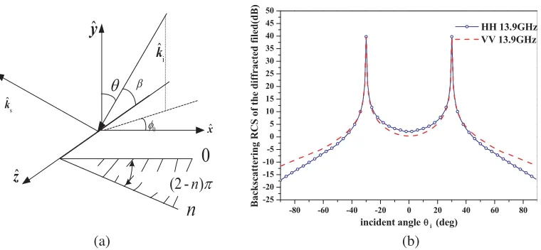
Figure 4. The wedge scattering. (a) Local coordinate system on the upper surface of the impedance wedge; (b) Backscattering RCS of the diffracted field of the 120◦ impedance wedge.

currents, retaining the contributions of the lower integral limit [33]. The incident field for H- and

V-polarizations expressed by the z-components of the electric and magnetic field take the following form

Ei_h= ezcosφ0+hzcosβ0sinφ0 sinβ0 (1−sin2β0sin2φ0)

e−jk·ˆr, Ei_v = −ezcosβ0sinφ0+hzcosφ0 sinβ0 (1−sin2β0sin2φ0)

e−jk·ˆr (23)

The surface currents can then be expressed as follows

⎧ ⎪ ⎪ ⎨ ⎪ ⎪ ⎩

Jx=v2[η+cosβ0cosφ0ez+ (η+sinφ0+ sinβ0)hz]

Jz =v2[(sinφ0+η+cosβ0)ez−cosβ0cosφ0hz]

Mx=v2[−η+(sinφ0+η+sinβ0)ez+ cosβ0cosφ0hz]

Mz _=v

2[η2+cosβ0cosφ0ez+η+(sinβ0+η+sinφ0)hz]

(24)

wherev2 = 2 sinφ0(1 +η+sinβsinφ)−1(η++ sinβsinφ)−1η+= 1/√εr.

The PO diffracted field due to the upper impedance face is as follows (sea Fig. 4(a))

EdP O=−

v1e−jk0ρsinβ0 2(cosφ+ cosφ0)

√

ρsinβ0

(ˆs׈s×J+ˆs×M)

η0HdP O=−

v1e−jk0ρsinβ0 2(cosφ+ cosφ0)

√

ρsinβ0

(ˆs׈s×M−ˆs×J)

(25)

We can obtain the PO diffraction coefficient

D11P O=b

!

−sinβ0sinφ0+η2+sinφsinβ0 −η+(sin2β0−sinφsinφ0−cosφ0cosφcos2β0)

"

D12P O=b{−η+cosβ0(sinφcosφ0−cosφsinφ0) + cosβ0sinβ0(cosφ0+ cosφ)}

D21P O=b

!

−η+2 sinβ0cosβ0(cosφ0+ cosφ) +η+(sinφcosβ0cosφ0−cosφcosβ0sinφ0)}

D22P O=b

!

sinβ0sinφ0−η+2 sinφsinβ0 −η+(sin2β−sinφsinφ0−cosφ0cosφcos2β0)

"

(26)

For the lower face, the required substitutions are η+ →η−, phi0 → nπ−φ0, φ→nπ−φ, β =π−β. We can obtain the incremental length diffraction coefficients (ILDC)Df by setting

Df =D−DP O (27)

The diffracted field can be expressed as

Ezd=

Df11Ezi +D f

12η0Hzi

ejkzcosβ e

jkρsinβ

ρ/sinβ

η0Hzd=

Df21Ezi +D f

22η0Hzi

ejkzcosβ e

jkρsinβ

ρ/sinβ

The equivalent edge currents can be derived as

Z0Ie=−

ejπ42√2πk k

D11f Ezi +D f

12η0Hzi

ejkzcosβ

Im =−e

jπ₄₂√_2πk

k

D21f E

i z+D

f

22η0Hzi

ejkzcosβ

(29)

The diffracted scattering field by a finite-length impedance wedge of arbitrary angles can then be obtained by integrating the equivalent edge currents

Ed=jkGr,r Z0Ie(r)ˆs׈s׈t+Im(r)ˆs׈t

·

L

ejkz(cosβ0+cosβp)

dl (30)

whereG(r,r) is the Green function,lthe impedance wedge path, andˆtthe unit vector along the wedge. The backscattering RCSs of the diffracted field of a single wedge for the HH and VV polarizations are compared in Fig. 4(b). The two peaks are caused by the specular reflection of the wedge plane. We can observe that the RCS for the HH polarization is higher than that for the VV polarization between the two peaks.

3.4. Foam Scattering

We assume that the breaking wave facet is covered by crest-foam, and the rough sea surface is covered by static-foam. Both the foam layers are composed of spherical particles with different thicknesses, which are discussed in Section 2.1. The geometry of foam above the sea surface scattering is shown in Fig. 5. According to [34], the solution of the VRT equation is obtained using an iterative method, and the zero-order as well as the corresponding first-order backscattering coefficient can be reduced to the following expressions for a two-scale random rough surface [16, 35]:

σpq(0)(θi) =σpq0(θi)e−2κedsecθi

σhh(1)(θi) =

3 4cosθi

κs

κe

1−e−2κedsecθi_×1+|R

h0|4×e−2κedsecθi

+3dκs|Rh0|2e−2kedsecθi

σvv(1)(θi) =

3 4cosθi

κs

κe

1−e−2κedsecθ_i×1+|

Rv0|2e−2κedsecθi

+3dκs |Rv0|2e−2κedsecθicos2(2θi)

(31)

where σpq0 is the backscattering coefficient of the local facet of the foam-free sea surface, andd is the thickness of foam layers. κs and κe are the scattering and extinction coefficients. Rh and Rv are the

Fresnel coefficients of the local facet, andθi is the local incident angle. For a sea surface with breaking

waves crest foam coverage and static foam coverage, the total scattering coefficient is given by

σ= 1

A

M

i=1

N

j=1

(1−Fs−Fc)σijsea+Fcσijf c+bw +Fsσijf s+sea

ΔxΔy (32)

whereA and ΔxΔy are the areas of the generated sea surface and single facet, respectively; Fs and Fc

are the static and crest-foam coverage, respectively. σsea

ij is the backscattering coefficient for a single

d

(a) (b)

facet of the sea surface, σf cij+bw the backscattering coefficient for a single facet of the sea surface with

breaking waves and crest foam, and σijf s+sea the backscattering coefficient for a single facet of the sea

surface with static foam.

3.5. SAR Imagery Simulations and Sea Clutter Distributions

After the development of the scattering process at low grazing angles, it is worthwhile to pay attention to the SAR image of the surface at a much finer resolution of grazing angles. Since we obtained the scattering coefficientσ(xg, yg) for each discrete facet, it is easy to simulate the ensemble averaged image

intensity through the velocity bunching (VB) model proposed by Alpers [36] in the following translation

I(x, y) =

Lx/2

−Lx/2

Ly/2

−Ly/2

dxgdygσI(xg, yg)fy(x−xg)

·ρaN/ρaN

exp

−π(y−yg−R·ur)/

ρaNV 2

(33)

where σI(xg, yg) =σ(xg, yg)(1 +fSAR(xg, yg)) denotes the backscattering coefficients (BSC) of the sea

surface that takes the tilt and velocity bunching into account. fSAR(xg, yg) is the velocity bunching

modulation function. ur is the orbital velocity in the range direction. Further,fy(x−xg) is the range

resolution function; ρaN = Nlρa denotes the stationary target azimuth resolution for Nl incoherent

looks; ρa=λR/2V T is the azimuth resolution; λ is the electromagnetic wavelength; V is the aircraft

velocity; T is the synthetic aperture duration; andρaN is the degraded azimuth resolution due to the

target acceleration and finite scene coherence time

ρaN =ρaN #

1 + 1

Nl $

πT2

λ ar(x

_{, y)}2₊T

τs

2%&1/2

(34)

wherear is the orbital acceleration in the range direction, andτs is the scene coherence time.

4. RESULTS AND DISCUSSIONS

Sea clutter can be described in terms of the statistical behavior of the returns from multiple distributed scatterer and individual discrete scatterer. In this section, we will discuss the statistical behavior and spatial properties of the backscatter from the sea surface with and without the breaking waves and foam layers.

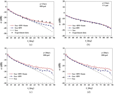
Figure 6 provides a comparison of the statistical characteristics of the backscattering coefficients (BSC), which are averaged over 50 samples of the sea surface with and without the breaking waves and foam layers, and the measured data [37] both for HH and VV polarizations at different wind speeds. During simulation, the frequency is set at 13.9 GHz; the wind speed at 10 m height is 13 m/s; the temperature is 20◦; the salinity is 35 ; and the permittivity for the seawater can be determined by the Two Debye model. We observe that the resonant scattering (without considering nonBragg scattering caused by the breaking wave and foam) from the sea surface for HH polarization is much less than that for VV polarization at a low grazing angle. When the breaking wave results are added into the composite model, the backscattering coefficients become significantly enhanced for HH polarization at LGA, and this is confirmed by the experiments. Furthermore, when foam effects are involved, the results of our model are more consistent with the measured data. These results are straightforward enough to interpret the sea spikes at LGA in terms of the scattering models described in Section 2. We observe that the BSC increases under high wind speed conditions for both polarizations, due to the roughness of the sea surface. We also find that the BSC increases obviously, especially for the HH polarizations at LGA incidence, which can be explained by the whitecap coverage increasing with high wind speed.

30 35 40 45 50 55 60 65 70 75 80 85 90 -50

-40 -30 -20 -10 0 10

Sea +BW+foam Sea+BW Sea

Experiment data

u=13m/s HH-pol

θ_i(deg)

σ

(dB)

30 35 40 45 50 55 60 65 70 75 80 85 90 -40

-30 -20 -10 0 10 20

Sea +BW+foam Sea+BW Sea

Experiment data

u=13m/s VV-pol

30 35 40 45 50 55 60 65 70 75 80 85 90 -50

-40 -30 -20 -10 0 10

u=20m/s HH-pol

Sea +BW+foam Sea +BW Sea

30 35 40 45 50 55 60 65 70 75 80 85 90 -50

-40 -30 -20 -10 0 10

u=20m/s HH-pol

Sea +BW+foam Sea +BW Sea

σ

(dB)

σ

(dB)

σ

(dB)

θ_i(deg)

θ_i(deg) θ_i(deg)

(a) (b)

(c) (d)

Figure 6. Backscattering coefficients (BSC) of the sea surface, the sea surface with breaking waves, the sea surface with breaking waves and foam, and the measured data. (a) HH-pol, u10 = 13 m/s; (b) VV-pol,u10= 13 m/s; (c) HH-pol,u10= 20 m/s; (d) VV-pol, u10= 20 m/s.

(c) (d)

(e) (f)

(g) (h)

2 4 6 8 10 12 14 16 18 20 22 24 26 28 30 -35 -30 -25 -20 -15 -10 -5 σ (dBsm) HH exp_data sea surface sea+BW+foam

θ_i=40ο

u₁₀(m/s)

2 4 6 8 10 12 14 16 18 20 22 24 26 28 30 -35 -30 -25 -20 -15 -10 -5 VV exp_data sea surface sea+BW+foam

θ_i=40ο

u₁₀(m/s)

2 4 6 8 10 12 14 16 18 20 22 24 26 28 30 -50 -45 -40 -35 -30 -25 -20 -15 -10 HH exp_data sea surface sea+BW+foam

u₁₀(m/s)

σ_i=55ο

2 4 6 8 10 12 14 16 18 20 22 24 26 28 30 -40 -35 -30 -25 -20 -15 -10 -5

u₁₀(m/s)

σ_i=55ο

VV exp_data sea surface sea+BW+foam

2 4 6 8 10 12 14 16 18 20 22 24 26 28 30 -60 -50 -40 -30 -20 -10

u₁₀(m/s)

HH exp_data sea surface sea+BW+foam σ_i=60ο

2 4 6 8 10 12 14 16 18 20 22 24 26 28 30 -44 -42 -40 -38 -36 -34 -32 -30 -28 -26 -24 -22 -20 -18 -16 -14 -12 -10-8

u₁₀(m/s)

VV exp_data sea surface sea+BW+foam

σ_i=60ο

σ (dBsm) σ (dBsm) σ (dBsm) σ (dBsm) σ (dBsm) (a) (b) (c) (d) (e) (f)

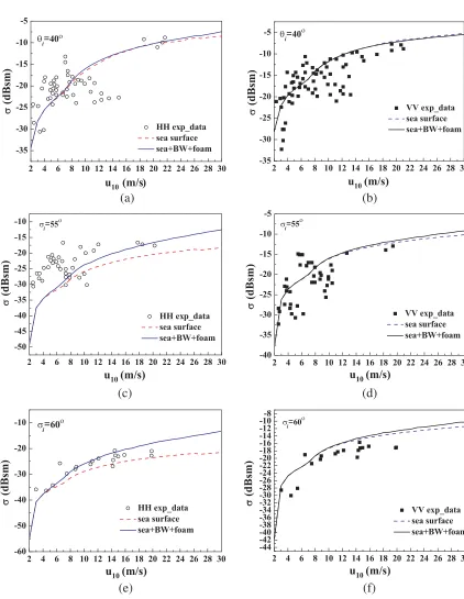
Figure 8. BSC of the sea with and without breaking waves and foam layers versus the wind speed for different incident angles. (a) HH-pol, θi= 40◦; (b)VV-pol,θi= 40◦; (c) HH-pol, θi = 55◦; (d) VV-pol,

θi= 55◦; (e) HH-pol, θi = 60◦; (f) VV-pol, θi = 60◦.

for HH polarization, whereas this phenomenon is not that obvious for VV polarization. We also find that there is a greater probability of large values for the BSC at higher wind speeds.

coverage increases significantly. This relationship is also reflected in the BSC results as shown in Fig. 8. The plotted curves go up with the increase of the wind speed and are less steep when the wind speed exceeds 15 m/s than those at medium wind speed (7–15 m/s), which can be explained as a limitation of the foam coverage. The BSCs versus wind speed are about the same level as the RADSCAT data with 40◦, 55◦ incidences, but the BSC is higher by 2 to 3 dB with 60◦ incidence for VV polarization. This bias was explained by [38], due to the calibration of the RADSCAT NRCS data and SASS data. These results clearly show that the contribution of breaking waves and volume scattering of foam layers

(a) (b)

(c) (d)

(g) (h)

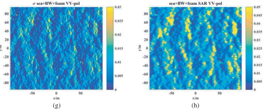
Figure 9. High-resolution SAR image of the sea surface simulated digitally. (a) BSC for sea surface; (b) SAR image intensity for sea surface; (c) BSC for sea surface with breaking waves and foam; (d) SAR image intensity for sea surface with breaking waves and foam; (e) BSC for sea surface; (f) SAR image intensity for sea surface; (g) BSC for sea surface with breaking waves and foam; (h) SAR image intensity for sea surface with breaking waves and foam.

is enhanced with increasing wind speed especially with large incidence.

Figure 9 presents the backscattering coefficients and simulated SAR images of the sea surface with and without breaking wave and foam layers for HH and VV polarizations. The SAR simulation parameters are τs = 0.3, T=0.18, R/V = 50, and Nl = 2. A clear phenomenon is observed wherein

the intensity enhancement for HH-pol is much larger than that for VV-pol corresponding to the region with breaking waves and foam layers; this is confirmed by the observation of the SAR images obtained from the along-track interferometric (ATI) SAR data collected along the North Carolina coast for the near shore breaking waves [40]. We also observe that the position of breaking waves in the SAR image is significantly shifted compared to its real position on the sea surface, and the resolution for the simulated SAR image is degraded both for HH and VV polarizations due to the orbital motion of the sea surfaces. When the breaking wave results and foam layers effects are taken into consideration, the backscattering coefficients are enhanced significantly especially for HH polarization, which is also reflected in the simulated SAR images. The image intensity from breaking wave patches and foam patches is enhanced compared to its counterpart from the sea surface patches for HH polarization. However, this phenomenon is less obvious for VV polarization due to the large background resonant scattering. The SAR image simulation can help to understand the signature of breaking waves and foam layers in a more realistic way.

5. CONCLUSIONS

The composite scattering models proposed earlier are not comprehensive enough to obtain the spatial distribution of the scattering characteristics of the deterministic sea surface with both breaking waves and foam layers. Thus, a volume-surface composite scattering model of nonlinear rough sea surfaces with breaking waves and foam layers driven by wind that is suitable for the microwave scattering at LGA is presented in this study.

Comparisons of our composite model with and without volume scattering for breaking waves and foam layers and experimental measurements with varying wind speeds and at 40◦, 55◦, and 60◦incidence are presented. These results clearly show that the contribution of breaking waves and volume scattering of foam layers is enhanced with the increase in wind speed especially with large incidence for HH polarizations.

Furthermore, the SAR images of sea surface with and without breaking waves and foam layers with an 80◦ incidence angle are simulated for HH and VV polarizations. The ensemble averaged image intensity from breaking wave patches and foam patches is enhanced compared to its counterpart from the sea surface patches for HH polarization. Further, the breaking point in the SAR image is significantly shifted compared with its real position on the sea surface.

Much work remains to be done on the detailed characterization of LGA scattering from the sea surface, i.e., (1) hydrodynamic theory for breaking waves [41] can also be invoked in our model to provide a better realization and data interpretation (2) cross-polarimetric scattering by calculating foam scattering coefficients directly through the integration for each facet in parallel is a technique that is promising. However, we believe that the main processes involved in the prediction of the scattering characteristics from the sea surface with breaking waves and foam layers have been fully considered in our model.

REFERENCES

1. Ward, K. D., R. J. A. Tough, and S. Watts, “Sea clutter: Scattering, the K distribution and radar performance,”Waves in Random and Complex Media, Vol. 17, No. 2, 233–234, 2007.

2. Luo, G. and M. Zhang, “Investigation on the scattering from one-dimensional nonlinear fractal sea surface by second-order small-slope approximation,” Progress In Electromagnetics Research, Vol. 133, 425–441, 2013.

3. Wei, P. B., M. Zhang, D. Nie, and Y. C. Jiao, “Improvement of SSA approach for numerical simulation of sea surface scattering at high microwave bands,”Remote Sens., Vol. 10, 1021, 2018. 4. Nie, D., M. Zhang, and N. Li, “Investigation on microwave polarimetric scattering from two-dimensional wind fetch- and water depth-limited nearshore sea surfaces,” Progress In Electromagnetics Research, Vol. 145, 251–261, 2014.

5. Li, X., B. Zhang, A. Mouche, Y. He, and W. Perrie, “Ku-band sea surface radar backscatter at low incidence angles under extreme wind conditions,” Remote Sens., Vol. 9, No. 5, 474–488, 2017. 6. Zhang, X. X., Z. S. Wu, and X. Su, “Influence of breaking waves and wake bubbles on surface-ship

wake scattering at low grazing angles,” Chin. Phys. Lett., Vol. 35, 074101, 2018.

7. Luo, W., M. Zhang, C. Wang, and H.-C. Yin, “Investigation of low-grazing-angle microwave backscattering from three dimensional breaking sea waves,”Progress In Electromagnetics Research, Vol. 119, 279–298, 2011.

8. Zhang, M., W. Luo, G. Luo, C. Wang, and H.-C. Yin, “Composite scattering of ship on sea surface with breaking waves,” Progress In Electromagnetics Research, Vol. 123, 263–277, 2012.

9. Melville, W. K. and P. Matusov, “Distribution of breaking waves at the ocean surface,” Nature, Vol. 417, 58–63, 2002.

10. Churyumov, A. N. and Y. A. Kravtsov, “Microwave backscatter from mesoscale breaking waves on the sea surface,”Waves Random Media, Vol. 10, 1–15, 2000.

11. Qi, C., Z. Zhao, W. Yang, Z.-P. Nie, and G. Chen, “Electromagnetic scattering and doppler analysis of three-dimensional breaking wave crests at low-grazing angles,” Progress In Electromagnetics Research, Vol. 119, 239–252, 2011.

12. West, J. C. and Z. Zhao, “Electromagnetic modeling of multipath scattering from breaking water waves with rough faces,” IEEE Transactions on Geoscience and Remote Sensing, Vol. 40, No. 3, 583–592, 2002.

14. Luo, W., M. Zhang, C. Wang, and H.-C. Yin, “Investigation of low-grazing-angle microwave backscattering from three-dimensional breaking sea waves,”Progress In Electromagnetics Research, Vol. 119, 279–298, 2011.

15. Luo, G., M. Zhang, and X.-F. Yuan, “Investigation of EM scattering from electrically large sea surface with breaking wave at low grazing angles,”Waves in Random and Complex Media, Vol. 23, No. 3, 226–242, 2013.

16. Wu, Z. S., J. P. Zhang, L. X. Guo, and P. Zhou, “An improved two-scale model with volume scattering for the dynamic ocean surface,” Progress In Electromagnetics Research, Vol. 89, No. 4, 39–56, 2009.

17. Fois, F., P. Hoogeboom, F. Le Chevalier, and A. Stoffelen, “Future ocean scatterometry: On the use of cross-polar scattering to observe very high winds,” IEEE Transactions on Geoscience and Remote Sensing, Vol. 53, No. 9, 5009–5020, 2015.

18. Wei, Y., L. Guo, and J. Li, “Numerical simulation and analysis of the spiky sea clutter from the sea surface with breaking waves,”IEEE Trans. Antennas Propag., Vol. 63, No. 11, 4983–4994, 2015. 19. Li, J., M. Zhang, W. Fan, and D. Nie, “Facet-based investigation on microwave backscattering from

sea surface with breaking waves: Sea spikes and SAR imaging,”IEEE Transactions on Geoscience and Remote Sensing, Vol. 55, No. 4, 2311–2325, 2017.

20. Wang, P., Y. Yao, and M. P. Tulin, “An efficient numerical tank for non-linear water waves, based on the multi-subdomain approach with BEM,”Int. J. Numer. Meth. Fl., Vol. 20, No. 12, 1315–1336, 1995.

21. Bonmarin, P., “Geometric properties of deep-water breaking waves,” J. Fluid Mech., Vol. 209, 405–433, 1989.

22. Coatanhay, A. and Y. M. Scolan, “Adaptive multiscale moment method applied to the electromagnetic scattering by coastal breaking sea waves,”Math Method Appl. Sci., Vol. 38, No. 10, 2041–2052, 2015.

23. Lyzenga, D. R., A. Maffett, and R. Shuchman, “The contribution of wedge scattering to the radar cross section of the ocean surface,”IEEE Transactions on Geoscience and Remote Sensing, Vol. 21, No. 4, 502–505, 1983.

24. Bondur, V. and E. Sharkov, “Statistical properties of whitecaps on a rough sea,” Oceanology, Vol. 22, 274–279, 1982.

25. Monahan, E. C. and D. K. Woolf, “Comments on variations of whitecap coverage with wind stress and water temperature,” J. phys. Oceanogr., Vol. 19, 706–709, 1989.

26. Reul, N. and B. Chapron, “A model of sea-foam thickness distribution for passive microwave remote sensing applications,”J Geophy. Res.: Oceans (1978–2012), Vol. 108, No. C10, 2003.

27. Voronovich, A. and V. Zavorotny, “Theoretical model for scattering of radar signals in Ku-and C-bands from a rough sea surface with breaking waves,” Waves Random Media, Vol. 11, No. 3, 247–269, 2001.

28. Anguelova, M. D., “Complex dielectric constant of sea foam at microwave frequencies,”J. Geophy. Res: Oceans, Vol. 113, No. C8, 2008.

29. Chen, H., M. Zhang, Y.-W. Zhao, and W. Luo, “An efficient slope-deterministic facet model for SAR imagery simulation of marine scene,”IEEE Trans. Antennas Propag., Vol. 58, No. 11, 3751– 3756, 2010.

30. Zhang, X., Z.-S. Wu, and X. Su, “Electromagnetic scattering from deterministic sea surface with oceanic internal waves via the variable-coefficient gardener model,” IEEE J — STARS, Vol. 11, No. 2, 355–366, 2018.

31. Cox, C., “Statistics of the sea surface derived from sun glitter,” J. Mar. Res., Vol. 13, 198–227, 1954.

33. Syed, H. H. and J. L. Volakis, “PTD analysis of impedance structures,” IEEE Trans. Antennas Propag., Vol. 44, 983–988, 1996.

34. Huang, X.-Z. and Y.-Q. Jin, “Scattering and emission from two-scale randomly rough sea surface with foam scatterers,” Proc. Inst. Elect. Eng. Microw. Antennas Propag., Vol. 142, 109–114, 1995. 35. Tsang, L. and J. A. Kong, Scattering of Electromagnetic Waves: Advanced Topics, John Wiley &

Sons, 2001.

36. Alpers, W. and C. Rufenach, “The effect of orbital motions on synthetic aperture radar imagery of ocean waves,” IEEE Trans. Antennas Propag., Vol. 27, No. 5, 685–690, 1979.

37. Plant, W. J., “Microwave sea return at moderate to high incidence angles,” Waves Random and Complex Media, Vol. 13, 339–354, 2003.

38. Schroeder, L., P. Schaffner, J. Mitchell, and W. Jones, “AAFE RADSCAT 13.9-GHz measurements and analysis: Wind-speed signature of the ocean,”IEEE J. Oceanic Eng., Vol. 10, 346–357, 1985. 39. Schroeder, L., W. Grantham, J. Mitchell, and J. Sweet, “SASS measurements of the Ku band radar

signature of the ocean,”IEEE J. Oceanic Eng., Vol. 7, 3–14, 1982.

40. Goncharenko, Y. V. and G. Farquharson, “In ATI SAR signatures of nearshore ocean breaking waves obtained from field measurements,”2013 IEEE International Geoscience and Remote Sensing Symposium (IGARSS), IEEE, Melbourne, VIC, Australia, 326–329, July 21–26, 2013.