Dimensionality Reduction for Text using Domain Knowledge

Dimensionality Reduction for Text using Domain Knowledge

Yi Mao and Krishnakumar Balasubramanian and Guy Lebanon

Georgia Institute of Technology

Abstract

Text documents are complex high dimen-sional objects. To effectively visualize such data it is important to reduce its di-mensionality and visualize the low dimen-sional embedding as a 2-D or 3-D scatter plot. In this paper we explore dimension-ality reduction methods that draw upon domain knowledge in order to achieve a better low dimensional embedding and vi-sualization of documents. We consider the use of geometries specified manually by an expert, geometries derived automat-ically from corpus statistics, and geome-tries computed from linguistic resources.

1 Introduction

Visual document analysis systems such as IN-SPIRE have demonstrated their applicability in managing large text corpora, identifying topics within a document and quickly identifying a set of relevant documents by visual exploration. The success of such systems depends on several fac-tors with the most important one being the qual-ity of the dimensionalqual-ity reduction. This is ob-vious as visual exploration can be made possible only when the dimensionality reduction preserves the structure of the original space, i.e., documents that convey similar topics are mapped to nearby regions in the low dimensional 2D or 3D space.

Standard dimensionality reduction methods such as principal component analysis (PCA), lo-cally linear embedding (LLE) (Roweis and Saul, 2000), or t-distributed stochastic neighbor embed-ding (t-SNE) (van der Maaten and Hinton, 2008) take as input a set of feature vectors such as bag of words. An obvious drawback is that such meth-ods ignore the textual nature of documents and in-stead consider the vocabulary wordsv1, . . . , vnas abstract orthogonal dimensions.

In this paper we introduce a framework for in-corporating domain knowledge into dimensional-ity reduction for text documents. Our technique does not require any labeled data, therefore is completely unsupervised. In addition, it applies to a wide variety of domain knowledge.

We focus on the following type of non-Euclidean geometry where the distance between documentxandyis defined as

dT(x, y) =

(x₋y)_{T(x−y). (1)}

HereT ∈Rn×n_{is a symmetric positive} semidef-inite matrix, and we assume that documentsx, y are represented as term-frequency (tf) column vectors. SinceT can always be written asHH for some matrix H ∈ Rn×n_{, an equivalent but} sometimes more intuitive interpretation of (1) is to compose the mappingx _→ Hx with the Eu-clidean geometry

dT(x, y) =dI(Hx, Hy) =Hx−Hy2. (2)

We can viewT as encoding the semantic similar-ity between pairs of words and H as smoothing the tf vector by mapping observed words to re-lated but unobserved words. Therefore, the geom-etry realized by (1) or (2) may be used to derive novel dimensionality reduction methods that are customized to text in general and to specific text domains in particular. The main challenge is to obtain the matricesH orT that describe the rela-tionship among vocabulary words appropriately.

HHdepends on the knowledge type and is dis-cussed in detail in Section 4.

We investigate the performance of the proposed dimensionality reduction methods for three text domains: sentiment visualization for movie re-views, topic visualization for newsgroup discus-sion articles, and visual exploration of ACL pa-pers. In each of these domains we evaluate the dimensionality reduction using several different quantitative measures. All the techniques men-tioned in this paper are unsupervised, making use of labels only for evaluation purposes.

Our take home message is that all three ap-proaches mentioned above improves dimension-ality reduction for text upon standard embedding (H = I). Furthermore, geometries obtained from corpus statistics are superior to manually constructed geometries and to geometries derived from standard linguistic resources such as Word-Net. Combining heterogenous types of knowl-edge provides the best results.

2 Related Work

Despite having a long history, dimensionality re-duction is still an active research area. Broadly speaking, dimensionality reduction methods may be classified as projective or manifold based (Burges, 2009). The first projects data onto a linear subspace (e.g., PCA and canonical corre-lation analysis) while the second traces a low di-mensional nonlinear manifold on which data lies (e.g., multidimensional scaling, isomap, Lapla-cian eigenmaps, LLE and t-SNE). The use of di-mensionality reduction for text documents is sur-veyed by Thomas and Cook (2005) who also de-scribe current homeland security applications.

Dimensionality reduction is closely related to metric learning. Xing et al. (2003) is one of the earliest papers that focus on learning metrics of the form (1). In particular they try to learn ma-trix T in an supervised way by expressing rela-tionships between pairs of samples. A representa-tive paper on unsupervised metric learning for text documents is Lebanon (2006) which learns a met-ric on the simplex based on the geometmet-ric volume of the data.

We focus in this paper on visualizing a cor-pus of text documents using a 2-D scatter plot. While this is perhaps the most popular and

prac-tical text visualization technique, other methods such as Spoerri (1993), Hearst (1997), Havre et al. (2002), Paley (2002), Blei et al. (2003), Mao et al. (2007) exist. Techniques developed in this paper may be ported to enhance these alternative visualization methods as well.

3 Non-Euclidean Geometries

Dimensionality reduction methods often assume, either explicitly or implicitly, Euclidean geome-try. For example, PCA minimizes the reconstruc-tion error for a family of Euclidean projecreconstruc-tions. LLE uses the Euclidean geometry as a local met-ric. t-SNE is based on a neighborhood structure, determined again by the Euclidean geometry. The generic nature of the Euclidean geometry makes it somewhat unsuitable for visualizing text docu-ments as the relationship between words conflicts with Euclidean orthogonality. We consider in this paper several alternative geometries of the form (1) or (2) which are more suited for text and com-pare their effectiveness in visualizing documents. As mentioned in Section 1, H smooths the tf vectorxby mapping the observed words into ob-served and non-obob-served (but related) words. In case H is nonnegative, it can be further decom-posed into a product of a non-negative column normalized matrixR _∈Rn×nand a non-negative diagonal matrixD ∈ Rn×n_{. The decomposition} H = RD shows that H has two key roles. It smooths related vocabulary words (realized byR) and it emphasizes some words over others (real-ized byD). Setting Rij to a high value ifwi, wj are similar and 0 if they are unrelated maps an observed word to a probability vector over re-lated words in the vocabulary. The valueDii cap-tures the importance ofviand therefore should be higher for important content words than for less important words or stop-words1.

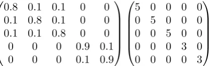
It is instructive to examine the matricesRand D in the case where the vocabulary words clus-ter in some meaningful way. Figure 1 gives an example where vocabulary words form two clusters. The matrix R may become block-diagonal with non-zero elements occupying di-agonal blocks representing within-cluster word

1

⎛ ⎜ ⎜ ⎜ ⎜ ⎝

0.8 0.1 0.1 0 0 0.1 0.8 0.1 0 0 0.1 0.1 0.8 0 0 0 0 0 0.9 0.1 0 0 0 0.1 0.9

⎞ ⎟ ⎟ ⎟ ⎟ ⎠

⎛ ⎜ ⎜ ⎜ ⎜ ⎝

5 0 0 0 0 0 5 0 0 0 0 0 5 0 0 0 0 0 3 0 0 0 0 0 3

⎞ ⎟ ⎟ ⎟ ⎟ ⎠

Figure 1: An example of a decompositionH = RDin the case of two word clusters_{v1, v2, v3}, {v4, v5}. The block diagonal elements inRrepresent the fact that words are mostly mapped to themselves, but sometimes are mapped to other words in the same cluster. The diagonal matrix indi-cates that the first cluster is more important than the second cluster for the purposes of dimensionality reduction.

blending, i.e., words within each cluster are in-terchangeable to some degree. The diagonal ma-trixDrepresents the importance of different clus-ters. The word clusters are formed with respect to the visualization task at hand. For example, in the case of visualizing the sentiment content of reviews we may have word clusters labeled as “positive sentiment words”, “negative sentiment words” and “objective words”.

In general, the matricesR, D may be defined based on the language or may be specific to docu-ment domain and visualization purpose. It is rea-sonable to expect that the words emphasized for visualizing topics in news stories might be dif-ferent than the words emphasized for visualizing writing styles or sentiment content.

Applying the geometry (1) or (2) to dimen-sionality reduction is easily accomplished by first mapping document tf vectorsx _→ Hxand pro-ceeding with standard dimensionality reduction techniques such as PCA or t-SNE. The resulting dimensionality reduction is Euclidean in the trans-formed space but non-Euclidean in the original space. In many cases, the vocabulary contains tens of thousands of words or more making the specification of T orH a complicated and error prone task. We describe in the next section several techniques for specifying these matrices in prac-tice.

4 Domain Knowledge

Method A: Manual Specification

In this method, a domain expert manually spec-ifies H = RD by specifying (R, D) based on the perceived relationship among the vocabulary

words. More specifically, the user first constructs a hierarchical word clustering that may depend on the current text domain, and then specifies the ma-trices(R, D)based on the clustering.

Denoting the clusters byC1, . . . , Cr(a partition of_{v1, . . . , vn}),Ris set to

Rij ∝

ρa, i=j, vi ∈Ca

ρab, i=j, vi ∈Ca, vj ∈Cb .

The valuesρab, a =bcapture the semantic simi-larity between two clusters and the valueρaa cap-tures the similarity of two different words within the cluster a. These values may be set manu-ally by domain expert or automaticmanu-ally computed based on the clustering hierarchy (for exampleρab can be the inverse of the minimal number of tree edges traversed in moving fromatob). To main-tain a probabilistic interpretation, the matrix R should be normalized so that its columns sum to 1. The diagonal matrixDis specified by setting the values

Dii=da, vi ∈Ca

according to the importance of word clusterCato the current visualization task.

We emphasize that as with the rest of the meth-ods in this paper, the manual specification is done without access to labeled data. Since manual clus-tering assumes some form of human intervention, it is reasonable to also consider cases where the user specifiesHorTin an interactive manner. For example, the expert specifies an initial clustering of words and values for(R, D), views the result-ing embeddresult-ings and adjusts the selection interac-tively until reaching a satisfactory embedding.

Method B: Contextual Diffusion

An alternative to manually specifying T =

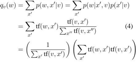
DRRDis to construct it based on similarity be-tween the contextual distributions of the vocabu-lary words. The contextual distribution of wordv is defined as

qv(w) =p(wappears inx|vappears inx) (3)

A natural similarity measure between distribu-tions is the Fisher diffusion kernel proposed by Lafferty and Lebanon (2005). Applied to contex-tual distributions as in Dillon et al. (2007) we ar-rive at the following similarity matrix

T(u, v) = exp

−carccos2

w

qu(w)qv(w)

.

wherec > 0. Intuitively, the worduwill be dif-fused intovdepending on the geometric diffusion between the distributions of likely contexts.

We use the following formula to estimate the contextual distribution from a corpus

qv(w) =

x

p(w, x_|v) =

x

p(w_|x, v)p(x_|v)

=

x

tf(w, x)tf(v, x)

xtf(v, x)

(4)

=

1

xtf(v, x) _x

tf(w, x)tf(v, x)

where tf(w, x)is the number of times wordw ap-pears in documentxdivided by the length of the documentx. The contextual distributionqvor dif-fusion matrixT above may be computed in an un-supervised manner without labels.

Method C: Webn-Grams

In method B the contextual distribution is com-puted using a large external corpus that is similar to the text being analyzed. An alternative that is especially useful when such a corpus is not eas-ily available is to use generic resources to esti-mate the contextual distribution (3)-(4). One op-tion is to use the publicly available Googlen-gram dataset (Brants and Franz, 2006) to estimate T. More specifically, we compute the contextual dis-tribution by considering the proportion of times two words appear together within the n-grams e.g., forn= 2we have

qv(w) =

#of bigrams containing bothwandv

#of bigrams containingv .

Method D: Word-Net

In the last method, we consider using Word-Net, a standard linguistic resource, to specifyT. This

Vocabulary

Sports

Others Canoeing catch boxing innings soccer

Team Name

Places

EU Asia

Mid east US Arizona francisco carolina atlanta austin

Others

Figure 2: Manually specified hierarchical word clustering for the 20 newsgroup domain. The words in the frames are examples of words belonging to several bottom level clusters.

is similar to manual specification (method A) in that it builds upon experts’ knowledge rather than corpus statistics. In contrast to method A, how-ever, Word-Net is a carefully built resource con-taining more accurate and comprehensive linguis-tic information such as synonyms, hyponyms and holonyms. On the other hand, its generality puts it at a disadvantage as method A may be adapted to a specific text domain.

We follow Budanitsky and Hirst (2001) who compared five similarity measures between words based on Word-Net. In our experiments we use the measure of Jiang and Conrath (1997) (see also Jurafsky and Martin (2008))

T(u, v) = log p(u)p(v) 2p(lcs(u, v))

as it was shown to outperform the others. Above, lcs stands for the lowest common subsumer, i.e., the lowest node in the hierarchy that subsumes (is a hypernym of) bothuandv. The quantity p(u)

is the probability that a randomly selected word in a corpus is an instance of the synonym set that contains wordu.

Combination of Methods

In addition to individual methods we also consider their convex combinations

H∗ =

i

αiHi s.t. αi ≥0,

i

αi = 1 (5)

and corpus statistics, leverage their diverse nature and potentially achieve better performance than any of the methods on its own.

5 Experiments

We evaluate the proposed methods by experiment-ing on two text datasets where domain knowledge is relatively easy to obtain (especially for method A and B). Preprocessing includes lower-casing, stop words removal, stemming, and selecting the most frequent 2000 words for both datasets.

The first is the Cornell sentiment scale dataset of movie reviews from 4 critics (Pang and Lee, 2004). The visualization in this case focuses on the sentiment quantity of either 1 (very bad) or 4 (very good) (Pang et al., 2002). For method A, we use the General Inquirer resource2to partition the vocabulary into three clusters conveying pos-itive, negative or neutral sentiment. While visu-alizing documents from one particular author, the rest of the reviews from other three authors can be used as an estimate of contextual distribution for method B.

The second text dataset is the 20 newsgroups. It consists of newsgroup articles from 20 distinct newsgroups and is meant to demonstrate topic vi-sualization. In this case one of the authors de-signed a hierarchical clustering of the vocabulary words based on general knowledge of English lan-guage (see Figure 2 for a partial clustering hier-archy) without access to labels. The contextual distribution for method B is estimated from the Reuters RCV1 dataset (Lewis et al., 2004) which consists of news articles from Reuters.com in the year 1996 and 1997.

Method C uses Googlen-gram which provides a massive scale resource for estimating the con-textual distribution. In the case of Word-Net (method D) we used Pedersen’s implementation of Jiang and Conrath’s similarity measure3. Note, for these two methods, the obtained information is not domain specific but rather represents gen-eral semantic relationships between words.

In our experiments below we focused on two di-mensionality reduction methods: PCA and t-SNE. PCA is a well known classical method while t-SNE (van der Maaten and Hinton, 2008) is a

re-2

http://www.wjh.harvard.edu/_∼inquirer/

3

http://wn-similarity.sourceforge.net/

cent dimensionality reduction technique for visu-alization purposes. The use of t-SNE is motivated by the fact that it was shown to outperform LLE, CCA, MVU, Isomap, and Laplacian eigenmaps when the dimensionality of the data is reduced to two or three.

To measure the dimensionality reduction qual-ity, we visualize the data as a scatter plot with dif-ferent data groups (topics, sentiments) displayed with different markers and colors. Our quantita-tive evaluation of the visualization is based on the fact that documents belonging to different groups (topics, sentiments) should be spatially separated in the 2-D space. Specifically, we used the follow-ing indices:

(i) The weighted intra-inter criteria is a standard

clustering quality index that is invariant to non-singular linear transformations of the embedded data. It equals tr(S_T−1SW)where SW is the within-cluster scatter matrix,ST = SW +SBis the total scatter matrix, andSB is the between-cluster scatter matrix (Duda et al., 2001).

(ii) The Davies Bouldin index is an alternative

to (i) that is similarly based on the ratio of within-cluster scatter to between-cluster scatter (Davies and Bouldin, 2000).

(iii) Classification error rate of ak-NN classifier that applies to data groups in the 2-D em-bedded space. Despite the fact that we are not interested in classification per se (other-wise we would classify in the original high dimensional space), it is an intuitive and in-terpretable measure of cluster separation.

(iv) An alternative to (iii) is to project the

em-bedded data onto a line which is the direc-tion returned by applying Fisher’s linear dis-criminant analysis to the embedded data. The projected data from each group is fitted to a Gaussian whose separation is used as a proxy for visualization quality. In particular, we summarize the separation of the two Gaus-sians by measuring the overlap area. While (iii) corresponds to the performance of a k-NN classifier, method (iv) corresponds to the performance of Fisher’s LDA classifier.

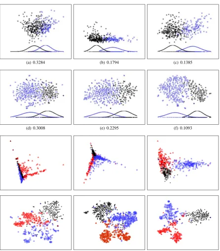
Figure 3 displays both qualitative and quanti-tative evaluation of PCA and t-SNE for the senti-ment and newsgroup domains forH =I(left col-umn), manual specification (middle column) and contextual distribution (right column). In general for both domains, methods A and B perform bet-ter both qualitatively and quantitatively (indicat-ing by the numbers in the top two rows) than the original dimensionality reduction with method B outperforming method A.

Tables 1-2 compare evaluation measures (i) and (iii) for different types of domain knowl-edge. Table 1 corresponds to the sentiment do-main where we conducted separate experiments for four movie critics. Table 2 corresponds to the newsgroup domain where two tasks were considered. The first involves three newsgroups (comp.sys.mac.hardware vs. rec.sports.hockey vs. talk.politics.mideast) and the second involves four newsgroups (rec.autos vs. rec.motorcycles vs. rec.sports.baseball vs. rec.sports.hockey). It is clear from these two tables that the contextual dif-fusion, Google n-gram, and Word-Net generally outperform the originalH = I matrix. The best method varies from task to task but the contextual diffusion and Googlen-gram in general result in good performance.

PCA (1) PCA (2) t-SNE (1) t-SNE (2)

H=I 1.5391 1.4085 1.1649 1.1206

B 1.2570 1.3036 1.2182 1.2331

C 1.2023 1.3407 0.7844 1.0723

D 1.4475 1.3352 1.1762 1.1362

PCA (1) PCA (2) t-SNE (1) t-SNE (2)

H=I 0.8461 0.5630 0.9056 0.7281

B 0.7381 0.6815 0.9110 0.6724

C 0.8420 0.5898 0.9323 0.7359

D 0.8532 0.5868 0.9013 0.7728

Table 2: Quantitative evaluation of dimensionality reduc-tion for visualizareduc-tion for two tasks in the news article domain. The numbers in the top five rows correspond to measure (i) (lower is better), and the numbers in the bottom five rows correspond to measure (iii) (k = 5) (higher is better). We conclude that contextual diffusion (B), Googlen-gram (C), and Word-Net (D) tend to outperform the originalH=I.

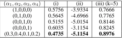
We also examined convex combinations

α1HA+α2HB+α3HC +α4HD (6)

with αi = 1 and αi ≥ 0. Table 3 displays quantitative results using evaluation measures (i), (ii) and (iii) where k is chosen to be 5 for (iii). The first four rows correspond to method A, B, C

(α1, α2, α3, α4) (i) (ii) (iii) (k=5) (1,0,0,0) 0.5756 -3.9334 0.7666 (0,1,0,0) 0.5645 -4.6966 0.7765 (0,0,1,0) 0.5155 -5.0154 0.8146 (0,0,0,1) 0.6035 -3.1154 0.8245 (0.3,0.4,0.1,0.2) 0.4735 -5.1154 0.8976

Table 3: Three evaluation measures (i), (ii), and (iii) (see the beginning of the section for description) for convex com-binations (6) using different values ofα. The first four rows represent methods A, B, C, and D. The bottom row repre-sents a convex combination whose coefficients were obtained by searching for the minimizer of measure (ii). Interestingly the minimizer also performs well on measure (i) and more impressively on the labeled measure (iii).

and D and the bottom row corresponds to a convex combination found which minimizes the unsuper-vised evaluation measure (ii) (i.e. the search for the optimal combination is based on (ii) that does not require labeled data). Note that the convex combination also outperforms method A, B, C, and D for measure (i) and more impressively for measure (iii) which is a supervised measure that uses labeled data. In general, by combining het-erogeneous types of domain knowledge, we may further improve the quality of dimensionality re-duction for visualization, and the search for such a combination may be accomplished without the use of labeled data.

Finally, we demonstrate the effect of domain knowledge on a new dataset that consists of all oral papers appearing in ACL 2001 – 2009. For the purpose of manual specification, we obtain 1545 unique words from paper titles, and as-sign for each word relatedness scores for the following clusters: morphology/phonology, syn-tax/parsing, semantics, discourse/dialogue, gen-eration/summarization, machine translation, re-trieval/categorization and machine learning. The score takes value from 0 to 2, where 2 represents the most relevant. The score information is then used to generate the transformation matrixR. We also assign for each word an importance value ranging from 0 to 3 (larger the value, more impor-tant the word). This information is used to gener-ate the diagonal matrixD.

(a) 0.3284 (b) 0.1794 (c) 0.1385

(d) 0.3008 (e) 0.2295 (f) 0.1093

Figure 3: Qualitative evaluation of dimensionality reduction for the sentiment domain (top two rows) and the newsgroup domain (bottom two rows). The first and the third rows display PCA reduction while the second and the fourth display t-SNE. The left column correspond to no domain knowledge (H =I) reverting PCA and t-SNE to their original form. The middle column corresponds to manual specification (method A). The right column corresponds to contextual diffusion (method B). Different groups (sentiment labels or newsgroup labels) are marked with different colors and marks.

Dennis Schwartz James Berardinelli Scott Renshaw Steve Rhodes

PCA t-SNE PCA t-SNE PCA t-SNE PCA t-SNE

H=I 1.8625 1.8781 1.4704 1.5909 1.8047 1.9453 1.8013 1.8415 A 1.8474 1.7909 1.3292 1.4406 1.6520 1.8166 1.4844 1.6610 B 1.4254 1.5809 1.3140 1.3276 1.5133 1.6097 1.5053 1.6145 C 1.6868 1.7766 1.3813 1.4371 1.7200 1.8605 1.7750 1.7979

H=I 0.6404 0.7465 0.8481 0.8496 0.6559 0.6821 0.6680 0.7410 A 0.6011 0.7779 0.9224 0.8966 0.7424 0.7411 0.8350 0.8513 B 0.8831 0.8554 0.9188 0.9377 0.8215 0.8332 0.8124 0.8324 C 0.7238 0.7981 0.8871 0.9093 0.6897 0.7151 0.6724 0.7726

Table 1: Quantitative evaluation of dimensionality reduction for visualization in the sentiment domain. Each of the four columns corresponds to a different movie critic from the Cornell dataset (see text). The top five rows correspond to measure (i) (lower is better) and the bottom five rows correspond to measure (iii) (k= 5, higher is better). Results were averaged over 40 cross validation iterations. We conclude that all methods outperform the originalH =Iwith the contextual diffusion and manual specification generally outperforming the others.

4 70 81 46 49 12 85 103 20 77 50 48 9 29 3 13 7 56 105 10 44 21 16

98 14 96 95 93 64 41 92 99 75 109 79 36 62 5 51 22 87 2 71 101 66 67 90

30 104 37 121 11 55 39 59 31 84 80 73 108 19 72 107 78 97 119 94 53 65 83 116 102 91 24 112 28 32 26 25 100 63 8 86 47 58 68 118 110 6 38 54

33 40 57 76 61 18 45 117 106 43 114113 60 15 27 34 74 88 69 89 42 17 115 82 111 23 120 35 52 4 70 81 46 49 12 85 103 20 77 50

48 9

29 3 13 7 56 105 10 44 21 16 98 14 96 95 93 64 41 92 99 75 109 79 36 62 5 51 22 87 2 71 101 66 67 90 30 104 37 121 11 55 39 59 31 84 80 73 108 19 72 107 78 97 119 94 53 65 83 116 102 91 24 112 28 32 26 25 100 63 8 86 47 58 68 118 110 6 38 54 33 40 57 76 61 18 45 117 106 43 114 113 60 15 27 34 74 88 69 89 42 17 115 82 111 23 120 35 52 4 70 81 46 49 12 85 103 20 77 50 48 9 29 3 13 7 56 105 10 44 21 16 98 14 96 95 93 64 41 92 99 75 109 79 36 62 5 51 22 87 2 71 101 66 67 90 30 104 37 121 11 55 39 59 31 84 80 73 108 19 72 107 78 97 119 94 53 65 83 116 102 91 24 112 28 32 26 25 100 63 8 86 47 58 68 118 110 6 38 54 33 40 57 76 61 18 45 117 106 43 114 113

60 15 27 34 74 88 69 89 42 17 115 82111 23 120 35 52

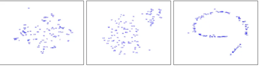
Figure 4:Qualitative evaluation of dimensionality reduction for the ACL dataset using t-SNE. Left: no domain knowledge (H=I); Middle: manual specification (method A); Right: contextual diffusion (method B). Each document is labeled by its assigned id from ACL anthology. See text for more details.

specifiedH(Figure 4 left) we get two clear clus-ters, the smaller containing papers dealing with machine translation and multilingual tasks. Inter-estingly, the contextual diffusion results in a one-dimensional manifold. Investigating the papers along the curve (from bottom to top) we find that it starts with papers discussing semantics and dis-course (south), continues to structured prediction and segmentation (east), continues to parsing and machine learning (north), and then moves to senti-ment prediction, summarization and IR (west) be-fore returning to the center. Another interesting insight that we can derive is the relative disconti-nuity between the bottom part (semantics and dis-course) and the rest of the curve. It seems spatial separability is higher in that area than in the other areas where the curve nicely traverses different re-gions continuously.

6 Discussion

In this paper we introduce several ways of incor-porating domain knowledge into dimensionality reduction for visualizing text documents. The

pro-posed methods all outperform in general the base-lineH = I, which is the one currently used in most text visualization systems.

References

Blei, D., A. Ng, , and M. Jordan. 2003. Latent dirich-let allocation. Journal of Machine Learning Re-search, 3:993–1022.

Brants, T. and A. Franz. 2006. Web 1T 5-gram Ver-sion 1.

Budanitsky, A. and G. Hirst. 2001. Semantic distance in wordnet: An experimental, application-oriented evaluation of five measures. In NAACL Workshop

on WordNet and other Lexical Resources.

Burges, C. 2009. Dimension reduction: A guided tour. Technical Report MSR-TR-2009-2013, Mi-crosoft Research.

Davies, D. L. and D. W. Bouldin. 2000. A cluster separation measure. IEEE Transactions on Pattern

Analysis and Machine Intelligence, 1(4):224–227.

Dillon, J., Y. Mao, G. Lebanon, and J. Zhang. 2007. Statistical translation, heat kernels, and expected distances. In Uncertainty in Artificial Intelligence, pages 93–100. AUAI Press.

Duda, R. O., P. E. Hart, and D. G. Stork. 2001. Pattern

classification. Wiley New York.

Havre, S., E. Hetzler, P. Whitney, and L. Nowell. 2002. Themeriver: Visualizing thematic changes in large document collections. IEEE Transactions on

Visu-alization and Computer Graphics, 8(1).

Hearst, M. A. 1997. Texttiling: Segmenting text into multi-paragraph subtopic passages. Computational

Linguistics, 23(1):33–64.

Jiang, J. J. and D. W. Conrath. 1997. Semantic sim-ilarity based on corpus statistics and lexical tax-onomy. In International Conference Research on

Computational Linguistics (ROCLING X).

Jurafsky, D. and J. H. Martin. 2008. Speech and

Lan-guage Processing. Prentice Hall.

Lafferty, J. and G. Lebanon. 2005. Diffusion kernels on statistical manifolds. Journal of Machine

Learn-ing Research, 6:129–163.

Lebanon, G. 2006. Metric learning for text docu-ments. IEEE Transactions on Pattern Analysis and

Machine Intelligence, 28(4):497–508.

Lewis, D., Y. Yang, T. Rose, and F. Li. 2004. RCV1: A new benchmark collection for text categorization research. Journal of Machine Learning Research, 5:361–397.

Mao, Y., J. Dillon, and G. Lebanon. 2007. Sequen-tial document visualization. IEEE Transactions on

Visualization and Computer Graphics, 13(6):1208–

1215.

Paley, W. B. 2002. TextArc: Showing word frequency and distribution in text. In IEEE Symposium on

In-formation Visualization Poster Compendium.

Pang, B. and L. Lee. 2004. A sentimental eduction: sentiment analysis using subjectivity summarization based on minimum cuts. In Proc. of the Association

of Computational Linguistics.

Pang, B., L. Lee, and S. Vaithyanathan. 2002. Thumbs up?: sentiment classification using machine learn-ing techniques. In Proc. of the Conference on

Em-pirical Methods in Natural Language Processing.

Roweis, S. and L. Saul. 2000. Nonlinear dimensional-ity reduction by locally linear embedding. Science, 290:2323–2326.

Spoerri, A. 1993. InfoCrystal: A visual tool for infor-mation retrieval. In Proc. of IEEE Visualization.

Thomas, J. J. and K. A. Cook, editors. 2005.

Illu-minating the Path: The Research and Development Agenda for Visual Analytics. IEEE Computer

Soci-ety.

van der Maaten, L. and G. Hinton. 2008. Visualiz-ing data usVisualiz-ing t-sne. Journal of Machine LearnVisualiz-ing

Research, 9:2579–2605.

Xing, E., A. Ng, M. Jordan, and S. Russel. 2003. Dis-tance metric learning with applications to clustering with side information. In Advances in Neural