DOI: 10.1534/genetics.108.089474
Modeling Multiallelic Selection Using a Moran Model
Christina A. Muirhead
1and John Wakeley
Department of Organismic and Evolutionary Biology, Harvard University, Cambridge, Massachusetts 02138 Manuscript received March 21, 2008
Accepted for publication May 18, 2009
ABSTRACT
We present a Moran-model approach to modeling general multiallelic selection in a finite population and show how it may be used to develop theoretical models of biological systems of balancing selection such as plant gametophytic self-incompatibility loci. We propose new expressions for the stationary distribution of allele frequencies under selection and use them to show that the continuous-time Markov chain describing allele frequency change with exchangeable selection and Moran-model reproduction is reversible. We then use the reversibility property to derive the expected allele frequency spectrum in a finite population for several general models of multiallelic selection. Using simulations, we show that our approach is valid over a broader range of parameters than previous analyses of balancing selection based on diffusion approximations to the Wright–Fisher model of reproduction. Our results can be applied to any model of multiallelic selection in which fitness is solely a function of allele frequency.
N
ATURAL selection has long been a topic of interest in population genetics, yet the stochastic theory of genes under selection remains underdeveloped com-pared to the theory of neutral genes. Due to the interplay of stochastic and deterministic forces, models of selection present analytical challenges beyond those of neutral models, although a great deal of progress has been made with models that use diffusion approxima-tions to a Wright–Fisher model of reproduction. Diffusion approximations with selection are, however, sometimes difficult to employ and always require assumptions about population parameters for tractabil-ity. These limitations suggest that there may be value in developing new methods of solving the problem of selection in a finite population, and here we do so using a Moran model of reproduction in place of the familiar Wright–Fisher model. Our approach has two major advantages over previous models: general applicability to a wide variety of selection models and accuracy over a broad range of parameter values. In this work, we propose new expressions for the full stationary distri-butions of allele frequencies under multiallelic selec-tion, as well as expressions for average allele frequency distributions.We restrict our attention to exchangeable models of selection, meaning that relabeling the alleles will not change selective outcomes and thus that selection will be a function of allele frequency rather than allele identity. Many models of selection can be transformed into frequency-dependent forms (Denniston and
Crow 1990), and some common models of selection have the desired property of exchangeability. For example, symmetric overdominant selection, in which heterozygotes have a selective advantage over homozy-gotes but the specific genotype of homozygote or heterozygote has no further selective effect, can be expressed as frequency-dependent selection on individ-ual (exchangeable) alleles, although the direct selec-tion is actually on diploid genotypes. Many other proposed models of multiallelic balancing selection, in which substantial variation is maintained by selec-tion, can be viewed in this way. Such models have been of particular interest because of the potential applica-tion to highly multiallelic systems found in nature, such as self-incompatibility (SI) loci in plants and the major histocompatibility complex (MHC) loci in vertebrates, and the desire to analyze these systems is a motivation for the present work. We now review some of the population genetic theory related to these systems.
Early in the history of population genetics, Wright (1939) presented a somewhat controversial stochastic model of gametophytic self-incompatibility (GSI) genes, sparking much further theoretical and empirical work. An analytic theory of multiallelic symmetric overdomi-nance was developed along similar lines to this early model (Kimuraand Crow1964; Takahata1990) and has been used as an approximation to the unknown mode of selection in the MHC (Takahataet al.1992). Drawing insights from these first two applications, other biological systems where balancing selection was posited, including sex determination in honeybees (Yokoyama and Nei1979), fungal mating systems (Mayet al.1999), and heterokaryon incompatibility in fungi (Muirhead et al.2002), have also been modeled successfully using
1Corresponding author: Department of Organismic and Evolutionary Biology, Harvard University, 16 Divinity Ave., Room 4100, Cambridge, MA 02138. E-mail: [email protected]
closely related approaches. Progress has been made in using these models to address genealogical (Takahata 1990; Vekemansand Slatkin1994) and demographic (Muirhead 2001) questions, as well as extending the models into more complex modes of selection (Uyenoyama2003) and reproduction (Vallejo-Marin and Uyenoyama2008).
Models of genetic variation under balancing selection have traditionally been focused on specific systems, such that extensions require entirely new analyses, and have also included a number of simplifying assumptions in the interest of mathematical tractability. For exam-ple, the symmetric overdominance model has been strongly criticized as an unrealistic approximation of MHC evolution (Patersonet al.1998; Hedrick2002; Penn et al. 2002; Ilmonen et al. 2007; Stoffels and Spencer2008), and yet it has proved difficult to make finite-population models of any of the more realistic frequency dependence schemes using the same ap-proaches. A constraint on further progress is the fact that the standard model of stochastic population genetics, the Wright–Fisher model, is in fact quite difficult to analyze.
The Wright–Fisher model of reproduction employs nonoverlapping generations, so that for a diploid population of size N, all 2N allele copies are chosen simultaneously when forming a new generation of individuals. While it is straightforward to describe this reproduction scheme mathematically as a discrete-time Markov chain, that chain unfortunately appears in-tractable even in simple cases (Ewens2004). Tradition-ally, then, diffusion approximations have been used to obtain quantities of interest, such as the equilibrium expected number of alleles, allele frequency spectra, and fixation probabilities and times. Diffusion approx-imations are derived in the limit N/‘, but are applicable to problems of finite N, provided that the strengths of other forces such as mutation and selection can be assumed to be weak, ofO(N1) (Ewens 2004). Watterson (1977) derived such a diffusion approxi-mation for multiallelic symmetric overdominance using these assumptions. More recently, as interest in popula-tion genetics has turned to problems of inference, Groteand Speed(2002) considered sampling proba-bilities under the diffusion approximation for symmet-ric overdominance, while Donnelly et al. (2001) and Stephens and Donnelly (2003) proposed computa-tional methods for some asymmetric models.
Although strong selection can be modeled using diffusion approximations by making the product of the population size and the selection coefficient (Ns) large, the assumption of weak selection is not in fact appropriate for the canonical biological systems of balancing selection. Specifically, selection coefficients are defined by the differences in fitness (the expected number of offspring) among individuals in the popula-tion at a given time. These differences may be large in
systems such as GSI, where the fitness of a very common allele may be very small while the fitness of other alleles may be greater than one.
In an attempt to deal with the extremely strong selection of gametophytic self-incompatibility, Wright’s (1939) original model focused attention on the dynam-ics of a single representative allele. He collapsed the influence of all other alleles into a single summary statistic: the homozygosity,F, which is a function of the frequencies of all alleles, and which Wright (1939) assumed to be constant. The analysis is essentially that of a two-allele system, using a one-dimensional diffusion analysis. This approach, while shown by simulation to be very effective in the appropriate parameter range (Ewensand Ewens1966), received substantial criticism on mathematical grounds (Fisher1958; Moran1962; Ewens1964b). Ewens(1964b), in particular, objected to the use of diffusion theory for GSI, pointing out that strong frequency-dependent selection violates the dif-fusion requirement that both the mean and the variance of the change in allele frequencies be small and of O(N1). Ewens(1964a) then applied Wright’s basic one-dimensional diffusion approach to modeling symmetric overdominance, but assumed that selection was weak and of O(N1) to stay within the strict limits of the diffusion approximation.
Kimura and Crow(1964) and Wright(1966), on the other hand, presented alternative one-dimensional diffusion approximations to symmetric overdominance, closer in spirit to Wright’s original model of GSI, that did not make the weak-selection assumption.
Watterson (1977) was concerned about both the
inconsistencies of the approximations used in these models and the treatment ofFas a constant rather than as a random variable dependent upon allele frequen-cies. Using his own multiallelic diffusion approximation for symmetric overdominance (Watterson1977), he derived an alternative (small-Ns) approximation to the frequency of a single representative allele. We consider this approximation, as well as the best-known one-dimensional symmetric overdominance diffusion, the strong-selection approximation of Kimura and Crow (1964), in comparison with our alternative approach to deriving allele frequency spectra under general multi-allelic selection with exchangeable alleles.
chain, without the need to resort to diffusion approx-imations. We exploit this trait to develop a new stochastic theory of multiallelic selection with minimal dependence on assumptions about population param-eter values. Our method has the additional benefit of being flexible: it can accommodate any exchange-able model of multiallelic selection and either of two general models of parent-independent mutation, the infinite-alleles and k-allele models of mutation. Our Moran-model predictions agree well with the results of Wright–Fisher simulations.
MODEL
We consider a general model of multiallelic selection, using a continuous-time Moran model of reproduction to incorporate random genetic drift. We explore in detail an infinite-alleles model of mutation, with selec-tion at either death (viability selecselec-tion) or reproducselec-tion (fecundity selection) and where selection depends only on the frequency of an allele, rather than its identity. Inappendix b, we present complementary results for a k-allele mutation model, also with two possible modes of exchangeable selection.
Structure of the Moran-model Markov chain: A single step in the Moran model corresponds to the death of one allele copy and the reproduction of one copy, possibly the same one chosen to die. Mutation may also occur during reproduction. Selection may be introduced at either point, and because it may be more convenient to use one or the other in specific biological situations, we formally develop separate models for selection at death and selection at reproduction. Re-gardless of when selection acts, we consider one step of the Moran model as consisting of one death event, followed by one reproduction/mutation event. The relative per-copy death rate of an allele ini copies is denotedmi, and the relative per-copy reproduction rate of ani-copy allele is denotedli. These determine the rates at which allele copies are chosen to die (in the selection-at-death version of the model) and to produce (in the selection-at-reproduction version), re-spectively. For death or reproduction events not affected by selection, allele copies are chosen to die or reproduce with equal probability regardless of type.
We imagine a diploid population of size N, so that there are a total of 2Nallele copies in the population. Under the infinite-alleles model of mutation, every new mutation produces a novel allele, and we assume that the probability that an allele copy mutates to a novel allele is u per reproduction event. The state of a population is recorded in a vector, X ¼ {X1, X2,. . .,
X2N}, whereXidenotes the number of alleles present ini copies. Thus, P2i¼N1iXi ¼2N. We are interested in the
state of the population at stationarity and consider both the full stationary distributionp(X)¼Pr[X1¼x1,X2¼
x2,. . .,X2N¼x2N] and the expected values both of the
random variablesXi, 1#i#2N, and of the productsXiXj for alliandj. The vector of expected numbers of alleles in each frequency class corresponds to the average allele frequency spectrum,f(x)dx, a classic object of popula-tion genetic theory usually obtained using diffusion approximations.
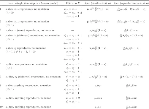
To analyze evolutionary dynamics, we construct a continuous-time Markov chain on X, the state vector describing the population. A single transition in this Markov chain corresponds to a single step of the Moran model, death followed by reproduction/mutation. The underlying Markov chain is complicated, in part be-cause the number of possible transitions that can be experienced by a particular X vector is very large. However, these transitions can be categorized into 10 distinct types depending on their effects onX(Table 1). To obtain the rate of a particular transition, we consider the two events in a step, death and reproduction, independently. For example, if in one step a copy from a 4-copy allele were picked to die, and a copy from a 10-copy allele were picked to reproduce (without muta-tion), this would represent a transition of type 5 withi¼ 4 andj¼10. The population will then have gone from stateX¼{x1,x2,x3,x4,. . .,x10,x11,. . .,x2N} to stateX9¼ {x1,x2,x311,x41,. . .,x101,x1111,. . .,x2N}. In the selection at death model, the rate of such a transition occurring, givenX, is
m44x4
10x10
2N ð1uÞ;
and the equivalent rate in the selection at reproduction model is
4x4
2Nl1010x10ð1uÞ:
With the 10 possible transition types and their effects on X as a complete description of the dynamics of the Markov chain, it is possible to derive equilibrium properties of the system, including stationary distribu-tions and average allele frequency spectra. We are able to obtain exact results for these quantities using the reversibility property of the Moran model with multi-allelic selection, which we now prove.
Stationary distributions and reversibility:Based on a product form of the stationary distribution of allele counts as in Moran(1962),e.g., see p. 134, we posit that the equilibrium distributions, p(X), of the population state vector under infinite-alleles mutation are of the form
pdðx1;x2;. . .;x2NÞ ¼Cd
Y2N i¼1
1 xi!
2Nu 1u
1 m1
Yi
m¼2 m1
mmm
" #xi
ð1Þ
prðx1;x2;. . .;x2NÞ ¼Cr Y2N
i¼1 1 xi!
2Nu
1ul0
Yi
m¼2
ðm1Þlm1 m
" #xi
ð2Þ
when selection occurs at reproduction. The normali-zation constants,CdandCr, are unknown functions of
selection and population parameters. These probabil-ity distributions are difficult to work with directly, in part because of the unknown constants, but they can be verified as correct, and used to show that their re-spective Markov chains are reversible, by a simple proof. With reversibility, at stationarity we have
pðXÞqðX;X9Þ ¼pðX9ÞqðX9;XÞ; ð3Þ
whereq(i,j) is the rate of transition from stateito state j in the chain. If our posited p-distributions satisfy all such relationships, the stationary distributions are verified, and the processes are reversible; see Theorem 1.3 in Kelly(1979).
Using Table 1, we can group transitions into classes that changeX in similar ways: type 1 and type 4 alter the counts in three adjacent elements, types 6 and 8 both alter x1 and two adjacent elements, types 7 and
9 alterx1andx2, and type 5 transitions alter two pairs
of (nonoverlapping) adjacent elements,xi1andxi, and
xjandxj11. Each one-step transition can be undone by
another one-step transition within the same class. For example, a type 1 transition withi¼6 is reversed by a type 4 transition withi¼5, and a type 6 transition with j¼5 is reversed by a type 8 transition withi¼6.
We can use these four transition classes to present a set of detailed balance equations (3) for the process at stationarity, and we use those balance equations to validate our posited stationary distributions and verify reversibility for the infinite-alleles mutation models in appendix a. We also present similar reversibility
argu-ments for ak-allele model of mutation, inappendix b. There we derive both stationary distributions analogous to (1) and (2) and average allele frequency spectra for
TABLE 1
Transition types in the infinite-alleles model of mutation
Event (single time step in a Moran model) Effect onX Rate (death selection) Rate (reproduction selection)
1 xidies,xi2reproduces, no mutation x9i2¼xi21 miixi
ði2Þxi2
2N ð1uÞ
ixi
2Nli2ði2Þxi2ð1uÞ
(i.2) x9i1¼xi112
x9i¼xi1
2 xidies,xi1reproduces, no mutation — miixi
ði1Þxi1
2N ð1uÞ
ixi
2Nli1ði1Þxi1ð1uÞ
(i.1)
3 xidies,xi(same) reproduces, no mutation — miixii
2Nð1uÞ
ixi
2Nliið1uÞ
4 xidies,xi(different) reproduces, no mutation x9i1¼xi111 miixi
iðxi1Þ
2N ð1uÞ
ixi
2Nliiðxi1Þð1uÞ
(i.1) x9i¼xi2
x9i11¼xi1111
5 xidies,xjreproduces, no mutation x9i1¼xi111 miixi
jxj
2Nð1uÞ
ixi
2Nljjxjð1uÞ
(i.1,j6¼i,i1,i2) x9i¼xi1
x9j¼xj1 x9j11¼xj1111
6 x1dies,xjreproduces, no mutation x91¼x11 m1x12jxNjð1uÞ 2xN1 ljjxjð1uÞ
(j6¼1) x9j¼xj1
x9j11¼xj1111
7 x1dies,x1(different) reproduces, no mutation x91¼x12 m1x1x21N1ð1uÞ 2xN1l1ðx11Þð1uÞ
x92¼x211
8 xidies, anything reproduces, mutation x91¼x111 miixiu 2ixNil02Nu
(i.1) x9i1¼xi111
x9i¼xi1
9 x2dies, anything reproduces, mutation x91¼x112 m22x2u 22xN2l02Nu
x92¼x21
10 x1dies, anything reproduces, mutation — m1x1u 2xN1 l02Nu
that mutation model, as we now do for infinite-alleles mutation.
Average allele frequency spectra: We begin our derivation of average allele frequency spectra with an identity,
X2N j¼1
jxj
2N ¼1;
which is true for every state vectorX¼{x1,x2,. . .,x2N}. Then, we have
xi ¼
X2N j¼1
jxj
2N xi:
Using a stationary distributionp(X) and taking expect-ations at equilibrium, this becomes
X
X
xipðXÞ ¼
X
X
X2N j¼1
jxj
2N xipðXÞ
E½Xi ¼
X2N j¼1
j
2N E½XiXj: ð4Þ
We derive the equilibrium expected valuesE[Xi] by first finding the expectations of the products E[XiXj] and then applying the equation above. The approach we use is to consider again the detailed balance equations and take expectations at stationarity, yielding a relatively simple system of equations relating the E[Xi]’s and E[XiXj]’s. This system of equations can then be solved numerically.
Selection at death: The first balance equation uses transitions of type 1 and type 4. The total expected rate of type 1 transitions at stationarity is
X
X
pdðXÞmiixi
ði2Þxi2
2N ð1uÞ
¼E½XiXi2mi
iði2Þ 2N ð1uÞ
and the total reverse rate of corresponding type 4 transitions (that would on average exactly undo the type 1 transitions above) is
X
X
pdðXÞmi1ði1Þxi1
ði1Þðxi11Þ
2N ð1uÞ
¼E½Xi1ðXi11Þmi1
ði1Þ2
2N ð1uÞ:
With reversibility these total rates are equal so that
E½XiXi ¼E½Xi1
mi11 mi
i1 i
i11
i E½Xi1Xi11; ð5Þ giving us our first expression for the relationship of the random variables Xi2, Xi1, and Xi. Two more such
expressions are necessary and are derived from two more balance equations. Balancing two type 5 transi-tions and taking expectatransi-tions gives
mi ij
2NE½XiXjð1uÞ
¼mj11ði1Þðj11Þ
2N E½Xi1Xj11ð1uÞ; wherei.1,j6¼i,i1,i2, so that
E½XiXj ¼
mj11 mi
ði1Þ
i
ðj11Þ
j E½Xi1Xj11; i,j: ð6Þ The last necessary pair required equates a type 6 transition and a type 8 transition for
miiE½Xiu¼m1
ði1Þ
2N E½X1Xi1ð1uÞ; fori.1, and thus
E½X1Xi ¼
mi11 m1
ði11Þ
i
2Nu
1uE½Xi11; i.1: ð7Þ Combining Equations 5–7, we have
E½XiXj ¼
i1j ij
2Nu 1u
Yi
r¼1
mj1r
mir11
!
E½Xi1j; i,j ð8Þ
E½XiXi ¼E½Xi1
2 i
2Nu 1u
Yi
r¼1
mi1r mir11
!
E½X2i: ð9Þ
From the identity (4) and Equations 8 and 9, we arrive finally at an expression for the average allele frequency spectrum under infinite-alleles mutation and selection at death:
E½Xi ¼
X Minði;2NiÞ
j¼1
i1j ið2N iÞ
2Nu
1u
Yj
r¼1 mi1r mjr11
! E½Xi1j
1 X
2Ni
j¼Minði;2NiÞ11 i1j ið2NiÞ
2Nu
1u
Yi
r¼1 mj1r mir11
! E½Xi1j:
ð10Þ While not a closed-form solution, this suffices to calculate numerically the vector ofE[Xi] values. We first calculate all terms recursively relative toE[X2N] and then normal-ize by P2i¼N1iE½Xi ¼2N. Note that once we have
com-puted expectations E[Xi], we can also compute Var[Xi] and Cov[XiXj], through use of (8)–(10). In addition, we can use the last element of the vector, E[X2N], to obtain the normalization constant Cdof the stationary
distribution pd(X), using E½X2N ¼PXx2NpdðXÞ ¼
pdð0;. . .; 0; 1Þ. With this, we now have a fully specified
stationary distribution (1) for the Markov chain. Selection at reproduction: Analysis for this model pro-ceeds along a very similar line to that for the previous model. The rates of the 10 types of transitions in this model are listed in the last column of Table 1, and reversibility of the process is formally verified in appen-dix a. We can use the same fundamental relation (4) for
of transitions as before and the transition rates for this model (Table 1), we find
E½XiXj ¼
i1j ij
2Nu 1u
Yi
r¼1
lir
lj1r1
!
E½Xi1j; i,j ð11Þ
E½XiXi ¼E½Xi1
2 i
2Nu 1u
Yi
r¼1
lir
li1r1
!
E½X2i ð12Þ
and
E½Xi ¼
X Minði;2NiÞ
j¼1
i1j ið2NiÞ
2Nu
1u
Yj
r¼1 ljr
li1r1 !
E½Xi1j
1 X
2Ni
j¼Minði;2NiÞ11 i1j ið2N iÞ
2Nu
1u
Yi
r¼1 lir
lj1r1 !
E½Xi1j
ð13Þ
so that we may calculateE[Xi] values as before.
RESULTS
Comparison to results from diffusion theory and simulations:We compare results from our approach to those from existing stochastic models of balancing selection, beginning with the well-studied case of sym-metric overdominance. Watterson (1977) assumed very weak selection to derive his multidimensional diffusion approximation to symmetric overdominance. In this case, weak means that the fitness advantage of heterozygotes,s, isO(N1). Analysis of the full diffusion model is impractical, and Watterson(1977) provided the following approximation for the expected one-dimensional allele frequency spectrum under an infin-ite-alleles model of mutation,
fðxÞ ux1ð1xÞu1 3
11sx½2 ð21uÞx
ð11uÞ
1 s
2x
2ð11uÞ2ð21uÞð31uÞ 3½8u1xð24132u14u2Þ
x2ð11uÞð48124u14u2Þ
1x3ð11uÞð24122u18u21u3Þ
;
which is valid for smalls¼2Nes, whereNeis the effective
population size, andu¼4Neu.f(x)dxis defined as the
equilibrium number of alleles expected in the fre-quency class (x,x1dx) and is equivalent to our vector of E[Xi] values with an appropriate dx. We have kept multiple terms in the Taylor expansion above to improve the accuracy of the approximation.
Kimuraand Crow(1964) assumed strong selection to obtain a different, one-dimensional, diffusion ap-proximation for multiallelic symmetric overdominance and infinite-alleles mutation:
fðxÞ CesðxFÞ2uxx1:
u and s are as before, except that in this model s represents the decrease in fitness of homozygotes. The random variableFis the homozygosity of the population (the sum of squared allele frequencies), which Kimura and Crow(1964) assumed to be a constant at equilib-rium under strong selection. When evaluating Kimura and Crow’s (1964) diffusion, instead of using one of the available closed-form approximations for the two unknown constants C and F (requiring additional assumptions), we used Mathematica 7.0 (Wolfram 2008) to numerically integrate the equations
ð1 0
xfðxÞdx¼1
and
ð1 0
x2fðxÞdx¼F;
solving simultaneously for C and F. The intent was to provide a solution that was minimally dependent on approximations beyond the assumptions inherent in the strong-selection, one-dimensional diffusion ap-proach itself.
To assess the accuracy of the Moran model approach developed here, relative to the Wright–Fisher model diffusions above, we performed extensive individual-based simulations of Wright–Fisher populations with symmetric overdominant selection and infinite-alleles mutation. The simulations use a discrete-time, non-overlapping generation framework, with reproduction and selection implemented as follows. In each genera-tion, tentative new diploid individuals are created by drawing two allele copies in a multinomial draw from the previous generation’s gamete pool (with each allele copy given a chance to mutate to a novel allele with probabilityu). The individual created is given a fitness value according to its genotype and is accepted or rejected as a member of the next generation according to the value of a random number drawn and compared to the fitness value. The process is repeated for all N individuals in each generation. Simulations were begun with triallelic populations and run for at least 100,000 generations, at which point allele frequencies were recorded. To ensure that the data were being sampled at stationarity, allele number and homozygosity were recorded at regular time points during the run. All sets of simulations appeared to have reached stationarity for average allele number and homozygosity by generation 20,000.
Comparisons between the Moran model and the Wright–Fisher model must account for the factor of 2 difference in timescale that results from differences in the distributions of the numbers of offspring per individual between these two modes of reproduction
Wright–Fisher diffusions, the Moran model prediction, and the simulation results adjust for this difference, as well as for the slight differences in the selection model between the two diffusion approximations. In all cases theNreported is theNof the Moran model, so that, for example, the corresponding Wright–Fisher simulation would be of a population of sizeN/2. Thesreported is thesof the following Moran model implementation of symmetric overdominance.
Symmetric overdominant selection in the Moran model is easily imposed through death-step selection. Allele copies in heterozygotes die at rate 1, and allele copies in homozygotes die at rate 1 1 s. Assuming Hardy–Weinberg proportions, a copy of an allele whose population frequency is i/2N will find itself in a homozygote with probabilityi/2Nand in a heterozygote with probability 1i/2N. This leads to
mi¼1 1 i 2N
1ð11sÞ i 2N
¼11s i 2N :
The sused here is equivalent to thes of the Kimura– Crow diffusion model.
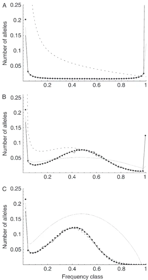
Figure 1 shows three comparisons between the simu-lations and the various analytic predictions for average allele frequency spectra. In Figure 1A (whereN¼2000, s¼0.001, andu¼105) selection is relatively weak (s¼ 2) and Watterson’s weak-selection diffusion (dotted line) tracks closely with the simulations (solid line, average of 10,000 iterations). The Moran model solution (thick dots) also tracks the simulations, while the Kimura–Crow strong-selection diffusion (dashed line) does not. In Figure 1C (where N ¼2000,s ¼0.01, and u ¼105), selection is strong (s¼20) and the Watterson diffusion no longer performs well, while the Kimura–Crow diffu-sion does. Again, the Moran model also accurately predicts the outcome of simulations. Figure 1B shows an intermediate situation (N¼2000,s¼0.005,u¼105) in which neither diffusion approximation is able to predict the results of the simulations, but the Moran model predicts simulation behavior very accurately.
Application to two specific types of selection: Plant self-incompatibility:GSI is a genetic system by which some plant species ensure outcrossing. A compatible mating can result when there are no alleles in common at the incompatibility locus (S locus) between haploid pollen (male gamete) and diploid stigma (female reproductive structure). For example, if a plant has diploid genotype AiAj at the S locus, its stigmas will express that diploid genotype and the ovules of the plant may be fertilized only by pollen bearing a different alleleAk, k6¼ i, j. Pollen expressingAiorAjlanding on anAiAjstigma will trigger an incompatibility reaction, so that no zygote will be formed. This type of mechanism, in a Moran model frame-work, naturally suggests selection at the reproduction
step. We approximate GSI by assuming that selection occurs only through the male part and that the re-productive success of an allele copy in pollen (relative to the success of a copy in a female gamete) is directly proportional to the frequency of diploid plants not containing that allele. Because all plants are hetero-zygotes under GSI, the frequency of plants containing an allele in frequencyi/2Nis simplyi/N. Thus, we can approximate the reproductive rate of an allele copy in frequencyi/2Nby
Figure1.—Correspondence between Moran and diffusion predictions and accuracy of predictions as assessed by simula-tions (averaged over 10,000 iterasimula-tions). Dotted line, Watter-son diffusion; dashed line, Kimura–Crow diffusion; thick dots, Moran solution; solid line, simulations. Symmetric
over-dominant selection is shown. Moran model parameters: (A)N¼
2000,s¼0.001,u¼105; (B)N¼2000,s¼0.005,u¼105;
li¼1 1
2 1 1
i N
1
2 ¼1 i
2N : ð14Þ
This approximation lacks some of the notable features of GSI. In particular, it does not require an overall number of alleles$3 (as required for a functional GSI system), and it does not restrict the allele frequencies to be#0.5 (which follows directly from the observation that all individuals in a GSI system must be hetero-zygotes). Nevertheless, this simple formulation per-forms well as judged by simulations.
The simulations shown in Figures 2 and 3 are again of Wright–Fisher (nonoverlapping generations) repro-duction with an appropriate population size conversion and in this case are individual-based simulations of gametophytic plant self-incompatibility under an infin-ite-alleles model of mutation. GSI was simulated by the following scheme: a diploid female parent and haploid pollen were picked randomly from the population and tested for compatibility. If they were compatible, a new zygote was generated from the possible gamete combi-nations; if incompatible, the pollen was discarded and a new pollen gamete picked until a compatible mating was achieved. Mutation to novel alleles occurred with probabilityuper gamete per generation.
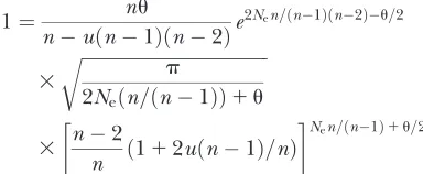
Figure 2 shows the average allele frequency spectrum predicted using the Moran approximation (14) for a population size ofN¼2000 and mutation rate ofu ¼ 106and compares it to the average spectrum obtained from forward simulations (25,000 iterations) and to the Wright–Fisher model diffusion prediction. The diffu-sion prediction was calculated following Uyenoyama’s
(2003) implementation of Wright’s model. Specifically, the effective number of common alleles (n) was ob-tained by solving
1¼ nu
nuðn1Þðn2Þe
2Nen=ðn1Þðn2Þu=2 3
ffiffiffiffiffiffiffiffiffiffiffiffiffiffiffiffiffiffiffiffiffiffiffiffiffiffiffiffiffiffiffiffiffiffiffiffiffiffiffiffiffip
2Neðn=ðn1ÞÞ1u
r
3 n2
n ð112uðn1Þ=nÞ
Nen=ðn1Þ1u=2
numerically and then substituting the resulting value of ninto the appropriate expression forf(x),
fðxÞ ¼ue2Nen2x=ðn1Þðn2Þð12xÞNen=ðn1Þ1u=21x1 (Uyenoyama 2003; Vallejo-Marin and Uyenoyama 2008).
Figure 3 compares the total number of alleles pre-dicted by both the Moran approach and the diffusion approximation to simulation results. To compute the total number of alleles predicted by the diffusion ap-proximation, we integrate f(x)dx over the allowable allele frequency range. Figure 3 shows that, in general, the Moran approximation tends to slightly underesti-mate the total number of alleles produced by simula-tions (100 iterasimula-tions for each point, box-and-whisker plot) unless the mutational input is extremely high, while the diffusion prediction follows a reverse pattern. Both estimates, however, fall within the ranges commonly seen in simulations for all parameter sets examined.
Figure2.—Accuracy of self-incompatibility approximation assessed by simulation: average allele frequency spectrum.
Solid line, Moran solution using (14) for N ¼ 2000, u ¼
106; dashed line, diffusion approximations for gametophytic
self-incompatibility,Ne¼1000,u¼106; dots, individual-based
simulations of a population (averaged over 10,000 indepen-dent iterations) with Wright–Fisher reproduction (nonover-lapping generations) and gametophytic self-incompatibility, Ne¼1000,u¼106.
Figure3.—Accuracy of self-incompatibility approximation assessed by simulation: allele number. Shaded triangles, ex-pected total number of alleles from the Moran solution for N¼1000 and mutation ratesu¼106, 105, 104, and 103;
shaded stars, expected total number of alleles from the
Wright–Fisher model diffusion approximation with Ne ¼
500 and the appropriate mutation rates. Simulation results, from individual-based forward simulations of a Wright–Fisher
population (Ne¼500) with gametophytic self-incompatibility,
A model of threshold frequency dependence: The Moran treatment of multiallelic selection is versatile and allows the study of any model in which the mode of selection is solely due to the frequency of an allele. Figure 4 shows the expected allele frequency spectrum for a very simple model of frequency dependence, in which selection depends on a critical threshold frequency. In this exam-ple, selection is applied at the reproduction step, such that
li¼ 1:0 if2iN ,0:1;
0:98 otherwise:
ð15Þ
The expected allele frequency spectrum is shown for this selection model (Figure 4, shaded line; see right-hand axis), withN ¼1000 and infinite-alleles mutation rate u¼105. The analytic prediction from the Moran model approach is represented by the solid line, and forward simulations (average of 25,000 iterations) are shown by dots. Simulations in this case were of a discrete-time Moran model of reproduction, where in each time step one allele copy was picked to die and one to reproduce and possibly mutate, as in the preceding analytic model. To run discrete-time simulations, we converted the reproduction rates given by (15) into per-time step probabilities, dividing by the total reproduction rate
P
ixili. The analytic prediction provides an accurate description of the consequences of this simple selection model. Analysis of additional complex selection models is equally straightforward with the analytic approach described above, limited only by the requirement that it must be possible to express an allele’s fitness as a function of its frequency, independent of allele identity.
DISCUSSION
The Moran approach to modeling multiallelic selec-tion has some immediate advantages over previous
methods based on diffusion analyses of Wright–Fisher models. Moran models can sometimes yield exact solutions where Wright–Fisher models cannot; in this case, the solution obtained is exact for a continuous-time model and appears to be an excellent approximation for discrete-time models such as those implemented in the Wright–Fisher model simulations. The exact solu-tions accurately portray the expected state of a popula-tion at equilibrium under selecpopula-tion across a range of parameters and modes of selection. The diffusion approximations based on the Wright–Fisher model, on the other hand, can falter when parameter values are outside their applicable ranges and have been developed only for a few well-studied modes of multiallelic selec-tion. Thus, although the diffusion approximations perform very well within their allowable parameter values, and with careful attention should yield accurate results, the Moran approach may be generally prefer-able. Additional simulations (not shown) demonstrate that thek-allele version of the Moran model with multi-allelic selection (appendix b) performs as well as the infinite-alleles version that is the focus of the diffusion comparisons, representing another extension of the applicability of the approach.
The traditional diffusion approximations have one significant practical advantage over the Moran ap-proach, in that the solutions, once obtained, tend to be easier to work with analytically. For example, while the expressions for the expected allele frequency spectra are exact in the continuous-time multiallelic Moran model, they are expressed as a system of equa-tions, rather than closed-form expressions as is possible for some of the one-dimensional diffusion approxima-tions. Moreover, the number of calculations required to obtain results from the Moran solution grows rapidly with population size N, making study of very large population sizes tedious and potentially vulnerable to inaccuracies due to machine precision limits. Neverthe-less, despite these difficulties resulting from the large size of the state space in an exact model, we believe that the disadvantages are outweighed by the advantages of having a more fully described stochastic model.
One biological system that could benefit from having a more complete stochastic description of allele dynam-ics is plant self-incompatibility, in which analysis has been hindered by the complexity of the selection mode. The good fit between the GSI simulations and our simple Moran model parameterization may be initially surprising, particularly in light of the realization that our parameterization (14) is algebraically equivalent to a simple model of overdominance with complete homo-zygote infertility. It has been pointed out (Vekemansand Slatkin 1994) that such a model underestimates the strength of selection in an SI system, and Wright’s more complicated analytic model of relative pollen success (Wright1939) has thus been favored in the study of GSI. Cases with low mutational input (Nu>1) show the Figure 4.—‘‘Threshold’’ frequency-dependent selection.
The fitness function (through differential rate of reproduc-tion) is plotted on the right axis (shaded line). On the left axis is the Moran model prediction for average allele fre-quency spectrum at equilibrium (solid line) and simulation
results (dots, average of 25,000 independent runs). N ¼
1000,u¼105. The simulations are of a population
expected apparently weaker selection of the Moran model approximation compared to full GSI simulations, through a smaller total number of alleles maintained (Figure 3) at higher frequency (Figure 2). The weakness of mutation is also evident in the lack of a low-frequency class in Figure 2. At higher mutational inputs (Nu.1), however, the Moran model actually overestimates the total number of alleles maintained by selection, appar-ently overestimating selection. A closer examination reveals that the discrepancy is due to the substantial number of alleles in the lowest (1-copy) frequency class in the Moran model, a frequency class that does not exist in simulations due to the transformationN¼2Ne.
Overall, however, the difference between simulation and either of the two analytic predictions is small. In fact, the average allele frequency spectrum obtained via the Moran approach seems to provide as good a match to simulations as does the diffusion prediction based on the more complicated (and biologically accurate) GSI approximation of Wright.
We explain this initially puzzling result by pointing out that the simulation method used (repeated pollen trials against a chosen female plant) is intuitively quite close to the Moran formulation of selection (females reproduce at rate one, males reproduce according to their probability of finding a compatible female plant). This is the standard simulation method for GSI (Mayo 1966; Yokoyamaand Nei1979; Vekemansand Slatkin 1994; Uyenoyama1997; Schierup1998; Schierupet al. 2000; Muirhead 2001), chosen in part via biological intuition (Mayo1966). The standard simulation meth-od has been an accepted way to mmeth-odel the complex selection in GSI; our results suggest that the simple Moran approach (or the algebraic equivalent, complete infertility of homozygotes) is an equally acceptable analytic model, at least for considering the quantities derived here, allele number and average allele fre-quency spectrum. The relationships among simula-tions, the Moran model analytic predicsimula-tions, and the Wright–Fisher diffusion analytic predictions are not constant across all population parameters, however, indicating a need for caution in the use of any analytic approach. Here again, however, the Moran model approach may be preferred because, with its limited set of approximations, it is relatively easy to isolate the causes of any discrepancies from simulations and to predict and account for other discrepancies in other parameter ranges.
The exact Moran approach for multiallelic selection may be helpful in studying other difficult systems of selection. Through its generality, it opens up a large number of selection models that were inaccessible (or, at least, unaccessed), using traditional diffusion meth-ods. An example is the fitness function shown in Figure 4, which while itself is quite simple (a threshold model with two alternative reproduction rates) yields a surpris-ingly complex expected allele frequency distribution.
As simple as this fitness model is, the work required to develop an appropriate diffusion approximation to its dynamics would be considerable, and simple adjust-ments to the model would require additional analysis. With the Moran model approach, due to reversibility, we have immediate access to the stationary distribution of allele frequencies, the equilibrium allele frequency spectrum, and related quantities for any exchangeable selection model,i.e., in which fitnesses depend only on allele frequencies.
The Moran model approach has been shown to provide a useful means of modeling a wide variety of fitness schemes, in particular those relevant to highly multiallelic systems of balancing selection. The ap-proach is minimally dependent on approximations and thus, unlike alternative methods, can be applied regard-less of the values of population parameters such as the strength of selection, mutation rate, and effective pop-ulation size. In addition to generating accurate expres-sions for the average allele frequency spectrum, using the Moran model yields fully specified expressions for p(X), the joint allele frequency spectrum, independent of the diffusion assumptions used to derive the standard results for multiallelic selection (first developed by Wright 1949). The expressions are general for any model of exchangeable multiallelic selection with par-ent-independent mutation, as are our proofs of revers-ibility of the underlying processes. We also obtained exact transition probabilities for all possible one-step transitions from a given population state X under any model of exchangeable selection. It is hoped that these results, by giving us a reasonably detailed picture of this class of complex stochastic processes, may prove useful in extending the analysis of multiallelic selection to prob-lems of ancestral inference, which has previously been restricted to a limited number of models of selection.
We are greatly indebted to Rick Durrett for many helpful comments and for suggesting a product form of the stationary distribution of allele frequencies that improved the work immensely. This work was supported by a Career Award (DEB-0133760) to J.W. from the National Science Foundation.
LITERATURE CITED
Denniston, C., and J. F. Crow, 1990 Alternative fitness models with
the same allele frequency dynamics. Genetics125:201–205. Donnelly, P., M. Nordborgand P. Joyce, 2001 Likelihoods and
simulation methods for a class of nonneutral population genetics models. Genetics159:853–867.
Ewens, W. J., 1964a The maintenance of alleles by mutation.
Genet-ics50:891–898.
Ewens, W. J., 1964b On the problem of self-sterility alleles. Genetics 50:1433–1438.
Ewens, W. J., 2004 Mathematical Population Genetics I. Theoretical
Intro-duction, Ed. 2. Springer-Verlag, New York.
Ewens, W. J., and P. M. Ewens, 1966 The maintenance of alleles
by mutation–Monte Carlo results for normal and self-sterility populations. Heredity21:371–378.
Feldman, M. W., 1966 On the offspring number distribution in a
genetic population. J. Appl. Probab.3:129–141.
Fisher, R. A., 1958 The Genetical Theory of Natural Selection.Dover,
Grote, M. N., and T. P. Speed, 2002 Approximate Ewens formulae
for symmetric overdominance selection. Ann. Appl. Probab.12:
637–663.
Hedrick, P. W., 2002 Pathogen resistance and genetic variation at
MHC loci. Evolution56:1902–1908.
Ilmonen, P., D. Penn, K. Damjanovich, L. Morrison, L. Ghotbi
et al., 2007 Major histocompatibility complex heterozygosity re-duces fitness in experimentally infected mice. Genetics 176:
2501–2508.
Kelly, F. P., 1979 Reversibility and Stochastic Networks. Wiley,
Chichester, UK.
Kimura, M., and J. F. Crow, 1964 The number of alleles that can be
maintained in a finite population. Genetics49:725–738. May, G., F. Shaw, H. Badraneand X. Vekemans, 1999 The
signa-ture of balancing selection: fungal mating compatibility gene evolution. Proc. Natl. Acad. Sci. USA96:9172–9177.
Mayo, O., 1966 On the problem of self-incompatibility alleles.
Bio-metrics22:111–120.
Moran, P. A. P., 1962 The Statistical Processes of Evolutionary Theory.
Clarendon Press, Oxford.
Muirhead, C. A., 2001 Consequences of population structure on
genes under balancing selection. Evolution55:1532–1541. Muirhead, C. A., N. L. Glassand M. Slatkin, 2002 Multilocus
self-recognition systems in fungi as a cause of trans-species polymor-phism. Genetics161:633–641.
Paterson, S., K. Wilsonand J. M. Pemberton, 1998 Major
histo-compatibility complex variation associated with juvenile survival and parasite resistance in a large unmanaged ungulate popula-tion (Ovis aries L.). Proc. Natl. Acad. Sci. USA95:3714–3719. Penn, D. J., K. Damjanovichand W. K. Potts, 2002 MHC
hetero-zygosity confers a selective advantage against multiple-strain in-fections. Proc. Natl. Acad. Sci. USA99:11260–11264.
Schierup, M. H., 1998 The number of self-incompatibility alleles in
a finite, subdivided population. Genetics149:1153–1162. Schierup, M. H., X. Vekemansand D. Charlesworth, 2000 The
effect of subdivision on variation at multi-allelic loci under bal-ancing selection. Genet. Res.76:51–62.
Stephens, M., and P. Donnelly, 2003 Ancestral inference in
popula-tion genetics models with selecpopula-tion. Aust. N. Z. J. Stat.45:395–430. Stoffels, R. J., and H. G. Spencer, 2008 An asymmetric model of
heterozygote advantage at major histocompatibility complex
genes: degenerate pathogen recognition and intersection advan-tage. Genetics178:1473–1489.
Takahata, N., 1990 A simple genealogical structure of strongly
bal-anced allelic lines and trans-species evolution of polymorphism. Proc. Natl. Acad. Sci. USA87:2419–2423.
Takahata, N., Y. Sattaand Y. Klein, 1992 Polymorphism and
bal-ancing selection at major histocompatibility complex loci. Genet-ics130:925–938.
Uyenoyama, M. K., 1997 Genealogical structure among alleles
reg-ulating self-incompatibility in natural populations of flowering plants. Genetics147:1389–1400.
Uyenoyama, M. K., 2003 Genealogy-dependent variation in viability
among self-incompatibility genotypes. Theor. Popul. Biol. 63:
281–293.
Vallejo-Marin, M., and M. K. Uyenoyama, 2008 On the
Evolution-ary Modification of Self-Incompatibility: Implications of Partial Clonality for Allelic Diversity and Genealogical Structure, pp. 53–71 inSelf-Incompatibility in Flowering Plants: Evolution, Diversity, and Mechanisms, edited by V. E. Franklin-tong. Springer-Verlag,
Berlin/Heidelberg, Germany.
Vekemans, X., and M. Slatkin, 1994 Gene and allelic genealogies
at a gametophytic self-incompatibility locus. Genetics137:1157– 1165.
Watterson, G. A., 1977 Heterosis or neutrality? Genetics85:789–
814.
Wolfram, S., 2008 Mathematica, Version 7.0. Wolfram Research,
Champaign, IL.
Wright, S., 1939 The distribution of self-sterility alleles in
popula-tions. Genetics24:538–552.
Wright, S., 1949 Adaptation and Selection, pp. 365–389 inGenetics,
Paleontology, and Evolution, edited by G. L. Jepsen, E. Mayrand
G. G. Simpson. Princeton University Press, Princeton, NJ.
Wright, S., 1966 Polyallelic random drift in relation to evolution.
Proc. Natl. Acad. Sci. USA55:1074–1081.
Yokoyama, S., and M. Nei, 1979 Population dynamics of
sex-deter-mining alleles in honey bees and self-incompatibility alleles in plants. Genetics91:609–626.
Communicating editor: M. K. Uyenoyama
APPENDIX A: REVERSIBILITY, INFINITE-ALLELES MODEL
To simplify notation, let
ai¼ 2Nu 1u
1 m1
Yi
m¼2 m1
mmm ðA1Þ
bi¼ 2Nu 1ul0
Yi
m¼2
ðm1Þlm1
m ðA2Þ
so that for our posited stationary distributions we have
pdðXÞ ¼Cd
Y2N i¼1
axi
i
xi!
ðA3Þ
and
prðXÞ ¼Cr
Y2N i¼1
bxi
i
xi!
: ðA4Þ
pdðXÞqðX;X9Þ ¼pdðX9ÞqðX9;XÞ
pdðXÞ pdðX9Þ
¼qðX9;XÞ
qðX;X9Þ: ðA5Þ
Leteibe the unit vector withxi¼1 and all other elements 0. From the transition types in Table 1, there are four possible detailed balances, with new population vectorsX9given by
X9¼X ei212ei1ei; i.2;
X9¼X1ei1eiej1ej11; i6¼1;j6¼i;i1;i2; X9¼X e1ej1ej11; j 6¼1;
X9¼X 2e11e2:
To further simplify notation in evaluating the detailed balances, letfdðxiÞ ¼axii=xi!. Then, for the first detailed balance in the selection at death model, we have
pdðXÞ pdðX9Þ ¼
fdðxi2Þ fdðxi21Þ
fdðxi1Þ fdðxi112Þ
fdðxiÞ
fdðxi1Þ
¼ai2
xi2
ðxi111Þðxi112Þ
a2
i1
ai
xi
¼mi1ði1Þðxi112Þði1Þðxi111Þ
miixiði2Þxi2
¼qðX9;XÞ
qðX;X9Þ: ðA6Þ
The last line holds because this balance equation equates two events, ‘‘death of ani-copy allele and reproduction of an (i2)-copy allele (no mutation),’’ which has transition rateq(X,X9)¼miixi((i2)xi2)(1u), and ‘‘death of an (i
1)-copy allele and reproduction of a different (i1)-copy allele (no mutation),’’ with rateq(X9,X)¼mi1(i1)(xi112)
((i1)(xi111)/2N)(1u).
We have three remaining detailed balances to verify for the selection at death model. Substituting as before into (A5), we have for the second balance equation, fori6¼1, andj6¼i,i1,i2,X9¼X1ei1eiej1ej11,
pdðXÞ
pdðX9Þ ¼
fdðxi1Þ fdðxi111Þ
fdðxiÞ
fdðxi1Þ
fdðxjÞ
fdðxj1Þ
fdðxj11Þ fdðxj1111Þ
¼ðxi111Þ ai1
ai xi
aj xj
ðxj1111Þ
aj11
¼mj11ðj11Þðxj1111Þði1Þðxi111Þ miixijxj
¼qðX9;XÞ
qðX;X9Þ; ðA7Þ
where the two events are ‘‘i-copy dies,j-copy reproduces, no mutation,’’ with rateq(X,X9)¼miixi(jxj/2N)(1u), and ‘‘(j11)-copy dies, (i1)-copy reproduces, no mutation,’’ with rateq(X9,X)¼mj11(j11)(xj1111)((i1)(xi111)/
2N)(1u).
pdðXÞ
pdðX9Þ ¼
fdðx1Þ fdðx11Þ
fdðxjÞ
fdðxj1Þ
fdðxj11Þ fdðxj1111Þ
¼a1
x1
aj xj
xj1111
aj11
¼mj11ðj11Þðxj1111Þ2Nu m1x1jxjð1uÞ
¼qðX9;XÞ
qðX;X9Þ; ðA8Þ
with the two events, ‘‘1-copy dies,j-copy reproduces, no mutation,’’ having rateq(X,X9)¼m1x1(jxj/2N)(1u), and
‘‘(j11)-copy dies, mutation,’’ with rateq(X9,X)¼mj11(j11)(xj1111)u.
The fourth detailed balance hasX9¼X2e11e2, yielding
pdðXÞ pdðX9Þ
¼ fdðx1Þ
fdðx12Þ fdðx2Þ fdðx211Þ
¼a1
x1
a1 ðx11Þ
ðx211Þ
a2 ¼ m22ðx211Þ2Nu
m1x1ðx11Þð1uÞ
¼qðX9;XÞ
qðX;X9Þ; ðA9Þ
where the two events are ‘‘1-copy dies, different 1-copy reproduces, no mutation,’’ with rateq(X,X9)¼m1x1((x11)/
2N)(1u), and ‘‘2-copy dies, mutation,’’ with rateq(X9,X)¼m22(x211)u. And
prðXÞqðX;X9Þ ¼prðX9ÞqðX9;XÞ prðXÞ
prðX9Þ ¼
qðX9;XÞ
qðX;X9Þ ðA10Þ
to verify the stationary distribution and reversibility of the process. For the first balance equation, we have for selection at reproduction,
prðXÞ prðX9Þ
¼ frðxi2Þ
frðxi21Þ
frðxi1Þ frðxi112Þ
frðxiÞ
frðxi1Þ
¼bi2
xi2
ðxi111Þðxi112Þ
b2
i1
bi xi
¼ði1Þðxi112Þli1ði1Þðxi111Þ
ixili2ði2Þxi2
¼qðX9;XÞ
qðX;X9Þ ðA11Þ
withq(X9,X) andq(X,X9) as before, with transition rates appropriate for selection at reproduction. For the second balance equation,
prðXÞ
prðX9Þ ¼
frðxi1Þ frðxi111Þ
frðxiÞ
frðxi1Þ
frðxjÞ
frðxj1Þ
frðxj11Þ frðxj1111Þ
¼ðxi111Þ bi1
bi xi
bj
xj
ðxj1111Þ
bj11
¼ðj11Þðxj1111Þli1ði1Þðxi111Þ
ixiljjxj
¼qðX9;XÞ
The third balance equation gives
prðXÞ prðX9Þ
¼ frðx1Þ
frðx11Þ frðxjÞ
frðxj1Þ
frðxj11Þ frðxj1111Þ
¼b1 x1
bj
xj
xj1111
bj11
¼ðj11Þðxj1111Þl02Nu
x1jljxjð1uÞ
¼qðX9;XÞ
qðX;X9Þ; ðA13Þ
and for the final detailed balance, we have
prðXÞ
prðX9Þ ¼
frðx1Þ frðx12Þ
frðx2Þ frðx211Þ
¼b1
x1
b1 ðx11Þ
ðx211Þ
b2 ¼ 2ðx211Þl02Nu
x1l1ðx11Þð1uÞ
¼qðX9;XÞ
qðX;X9Þ: ðA14Þ
This completes the reversibility proof for the infinite-alleles model with selection at reproduction and validates the posited stationary distribution (2).
APPENDIX B:k-ALLELE MUTATION
Stationary distributions and reversibility: We now consider the case ofk-allele mutation. In this model, there arek possible allelic types, and the probability of mutation to a particular type isu/k, independent of the ‘‘parental’’ type, for each reproduction event. Analysis of thek-allele model is similar to that of the infinite-alleles model, with some important departures. The population state vectorXnow includes a termx0, representing the number of thekpossible alleles not
present in the population (i.e., those having zero copies). There are, as in the infinite-alleles models, 10 basic types of transitions possible from a givenXvector, but because of the different role of mutation, these transitions are not the same as in the previous model. Because of the more consistent role of mutation in affecting alleles in different frequency classes, there are fewer special cases among the transitions that change the population state. We need to consider only two detailed balances: one in which death and reproduction occur to copies in nonoverlapping frequency classes (affecting i,i1,j, andj11,i6¼0 andj6¼i,i1,i2) and one in which reproduction and death affect a common frequency class, similar to paired transitions 1 and 4 in the infinite-alleles model. Formally, the twoX9vectors we must consider are
X9¼X1ei1eiej1ej11; i 6¼0;j6¼i;i1;i2
and
X9¼X ei212ei1ei; i.1:
We again suggest expressions for the stationary distributions,
pkdðx0;x1;. . .;x2NÞ ¼Ckd
Y2N i¼0
1 xi!
Yi
m¼1
ððm1Þ=2NÞð1uÞ1u=k mmm
" #xi
ðB1Þ
for selection at death and
pkrðx0;x1;. . .;x2NÞ ¼Ckr
Y2N i¼0
1 xi!
Yi
m¼1
lm1ðððm1Þ=2NÞð1uÞ1u=kÞ m
" #xi
ðB2Þ
for selection at reproduction, whereCkdandCkragain represent normalization constants. Reversibility can be verified
ai¼Y
i
m¼1 Rm1
mmm ðB3Þ
bi¼Y
i
m¼1
lm1Rm1
m ; ðB4Þ
where we have definedRias
Ri¼
i
2Nð1uÞ1 u
k: ðB5Þ
We also usefd(xi) andfr(xi) as before in the infinite-alleles model.
For the first balance equation we have, withX9¼X1ei1eiej1ej11,
pkdðXÞ pkdðX9Þ
¼ fdðxi1Þ
fdðxi111Þ fdðxiÞ
fdðxi1Þ
fdðxjÞ
fdðxj1Þ
fdðxj11Þ fdðxj1111Þ
¼ðxi111Þ ai1
ai xi
aj xj
ðxj1111Þ
aj11
¼mj11ðj11Þðxj1111Þðxi111ÞRi1 miixixjRj
¼qðX9;XÞ
qðX;X9Þ: ðB6Þ
Here the forward event is ‘‘ani-copy allele dies, and a new copy of aj-copy allele is created (through reproduction or mutation),’’ with rateq(X,X9)¼miixixjRj, and the reverse event is ‘‘a (j11)-copy allele dies, and a new copy of an (i 1)-copy allele is created (through reproduction or mutation),’’ with rate q(X9, X)¼ mj11(j 1 1)(xj11 1 1)
(xi111)Ri1.
For the second balance,X9¼Xei212ei1ei, and with selection at death,
pkdðXÞ pkdðX9Þ ¼
fdðxi2Þ fdðxi21Þ
fdðxi1Þ fdðxi112Þ
fdðxiÞ
fdðxi1Þ
¼ai2
xi2
ðxi111Þðxi112Þ
a2i1
ai xi
¼mi1ði1Þðxi112Þðxi111ÞRi1
miixixi2Ri2
¼qðX9;XÞ
qðX;X9Þ: ðB7Þ
The events here are ‘‘i-copy dies, and an (i2)-copy is created (through reproduction or mutation),’’ with rateq(X, X9) ¼ miixixi2Ri2, and ‘‘(i 1)-copy dies, and a (different) (i 1)-copy is created (through reproduction or
mutation),’’ with rateq(X9,X)¼mi1(i1)(xi112)(xi111)Ri1.
This completes the reversibility proof for selection at death withk-allele mutation. The proof for the selection at reproduction case is similar, using the same balance equations. We have, for the first balance equation,
pkrðXÞ pkrðX9Þ ¼
frðxi1Þ frðxi111Þ
frðxiÞ
frðxi1Þ
frðxjÞ
frðxj1Þ
frðxj11Þ frðxj1111Þ
¼ðxi111Þ bi1
bi xi
bj
xj
ðxj1111Þ
bj11
¼ðj11Þðxj1111Þli1ðxi111ÞRi1
ixiljxjRj
¼qðX9;XÞ
qðX;X9Þ: ðB8Þ
pkrðXÞ pkrðX9Þ
¼ frðxi2Þ
frðxi21Þ
frðxi1Þ frðxi112Þ
frðxiÞ
frðxi1Þ
¼bi2 xi2
ðxi111Þðxi112Þ
b2i1
bi xi
¼ði1Þðxi112Þli1ðxi111ÞRi1
ixili2xi2Ri2
¼qðX9;XÞ
qðX;X9Þ; ðB9Þ
verifying the posited stationary distributions and reversibility in the Moran model of selection at reproduction under a k-allele model of mutation.
Average allele frequency spectra:To obtain the equilibrium expectations forX, we begin again with the identity (4),
E½Xi ¼
X2N j¼1
j
2N E½XiXj;
and focus on finding expressions for the cross-productsE[XiXj]. Using the transitions in the first detailed balance above and taking expectations gives us, for the selection at death case,
miiE½XiXjRj¼mj11ðj11ÞE½Xj11Xi1Ri1; i.0;j6¼i;i1;i2
so that, fori,j
E½XiXj ¼
j11 i
mj11 mi
Ri1 Rj
E½Xi1Xj11: ðB10Þ
We also have from the other set of detailed balances that
miiE½XiðXi1ÞRi ¼mi11ði11ÞE½Xi11Xi1Ri1
fori.1 or
E½XiXi ¼E½Xi1
i11 i
mi11
mi Ri1
Ri
E½Xi1Xi11: ðB11Þ
Combining (B10) and (B11), we have
E½XiXj ¼
Yi
r¼1 j1r ir11
mj1r
mir11 Rir
Rj1r1
!
E½X0Xi1j; i,j ðB12Þ
E½XiXi ¼E½Xi1
Yi
r¼1 i1r ir11
mi1r
mir11 Rir
Ri1r1
!
E½X0X2i; ðB13Þ
leading to
E½Xi ¼
X
Minði;2NiÞ
j¼1 j 2N i
Yj
r¼1 i1r jr11
mi1r mjr11
Rjr
Ri1r1
!
E½X0Xi1j
1 X
2Ni j¼Minði;2NiÞ11
j 2N i
Yi
r¼1 j1r ir11
mj1r
mir11 Rir
Rj1r1
!
E½X0Xi1j: ðB14Þ
These expressions are more complex than in the infinite-alleles case, and it appears that in addition to the problem of finding the set of 2N 11E[Xi] elements, we have also set ourselves the task of first finding the set ofE[X0Xi]
x0 ¼k
X2N j¼1
xj;
and therefore
x0xi ¼kxi
X2N j¼1
xixj:
Then, taking the usual equilibrium expectations,
E½X0Xi ¼kE½Xi
X2N j¼1
E½XiXj: ðB15Þ
We then have
E½X0Xi ¼ ðk1ÞE½Xi
X
Minði;2NiÞ
j¼1
Yj
r¼1 i1r jr11
mi1r mjr11
Rjr
Ri1r1
!
E½X0Xi1j
X
2Ni
Minði;2NiÞ11
Yi
r¼1 j1r ir11
mj1r
mir11 Rir
Rj1r1
!
E½X0Xi1j: ðB16Þ
We have now expressedE[X0Xi] in terms of the ‘‘higher’’ vector elementsE[X0Xi1j], just as we were able to express
E[Xi] in terms of the higherE[Xi1j] in the infinite-alleles model. In that case, we obtained results by calculating all E[Xi] terms beginning withE[X2N] and moving down the vector, relative toE[X2N], and then normalizing to obtain E[X2N]. Here, our procedure is very similar, but with an added layer of calculation as we move down the vector to calculate theE[X0Xi]’s relative toE[X0X2N]. The procedure is straightforward becauseE[X0X2N]¼(k1)E[X2N], and thus we can calculate all theE[X0Xi]’s, as well asE[Xi], relative toE[X2N], and normalize at the end as before. The full expression forE[Xi] obtained in this manner is cumbersome, but a computer program can calculate the values readily. As in the infinite-alleles model, once we have the expectationsE[Xi], we can immediately calculate the normalization constantCkd, as well as Var[Xi] and Cov[XiXj] for thek-allele model.
Analysis ofk-allele mutation and reproduction-step selection is very similar, using the familiar balance equations and the appropriate transition rates. The expression for the cross-product expectations in the case of selection at reproduction is
E½XiXj ¼
Yi
r¼1 j1r ir11
lir
lj1r1 Rir
Rj1r1
!
E½X0Xi1j; i,j ðB17Þ
E½XiXi ¼E½Xi1
Yi
r¼1 i1r ir11
lir
li1r1 Rir
Ri1r1
!
E½X0X2i ðB18Þ
and we again use (B15) to obtain
E½X0Xi ¼ ðk1ÞE½Xi
X
Minði;2NiÞ
j¼1
Yj
r¼1 i1r jr11
ljr
li1r1 Rjr
Ri1r1
!
E½X0Xi1j
X
2Ni
Minði;2NiÞ
Yi
r¼1 j1r ir11
lir
lj1r1 Rir
Rj1r1
!
E½X0Xi1j: ðB19Þ