352 |
P a g e
Holographic Image Compression using
New Biorthogonal Wavelets
N. Hyndavi
1, T. Aruna
2 1PG Scholar, Dept. of ECE, GKCE, Sullurpet
2Assistant Professor, Dept. of ECE, GKCE, Sullurpet
ABSTRACT
Digital holography refers to the acquisition and processing of holographs. Image rendering, or reconstruction
of object data is performed numerically from digitized interferograms. Digital holography offers a means of
measuring optical phase data and typically delivers three-dimensional surface or optical thickness images.
Several recording and processing schemes have been developed to assess optical wave characteristics such as
amplitude, phase, and polarization state, which make digital holography a very powerful method for metrology
applications. With the invent of wavelet based coding schemes like Embedded Zerotree Wavelet and Set Partitioning in Hierarchical Trees, the image compression and image processing community as a whole has taken a turn to the study of wavelet analysis. Defining a suitable wavelet involves the shape, size and also the number of the basis functions. The important features of basis functions are vanishing moments, size of support, regularity and etc. Towards this end in this research work, the features of basis functions will be explored to find an optimal mother wavelet to be used in digital holography. In this paper, biorthogonal wavelets are explored and new variations are built and proved that the performance is superior to many existing ones.
Keywords:Spline function, image compression, biorthogonal wavelet, basis functions,
holographic images
I.INTRODUCTION
Consider wavelet transformation of an image for compression. Discrete wavelet transform will be applied to the image; the result of this transformation is wavelet coefficients or what is called wavelet domain. The transformation actually transforms the less correlated data to highly correlated data. When the inverse transform is applied directly on the transformed coefficients the original signal should be restored. Otherwise the transformation should not be used. This condition is called perfect reconstruction. All well-known wavelet transforms satisfy this condition [1][2].
353 |
P a g e
spatial domain image (generally deteriorated) is obtained. The aim of compression is to get a close reconstructed image (with original image) using few wavelet coefficients (or very less amount of memory). But this is very tough to maintain two things at a time because fundamentally these are inversely related [4].All well-known wavelets satisfy perfect reconstruction condition, i.e., when we apply inverse wavelet transform directly on wavelet domain of the image we get exact original image. But when coding is applied on the wavelet domain the reconstructed image is different from original image and also it is different for different wavelet bases. So, the error between original and reconstructed image and size of coded wavelet coefficients depends on the wavelet bases used [5][6]. The wavelet bases are characterized by using parameters like vanishing moments, compact support, regularity, etc. Also compared to the orthogonal wavelets the biorthongoal wavelet system is flexible with more design options. Hence in this research new biorthogonal bases will be designed with the optimal wavelet bases for image compression in mind.
II.DESIGN OF BIORTHOGONAL WAVELETS
The design of biorthogonal wavelet is concerned in generating two sets of functions with certain properties. The two sets are supposed to be used one in decomposition and other in reconstruction phase of wavelet transform [7].
0 ,
)
(
~
)
(
t
t
k
dt
k
n
k
k
n
h
n
h
(
)
~
(
2
)
,0(1)
i.e., h(n) is orthogonal to even translates of itself. Here
h
~
is orthogonal to h. Now let the
positioning of
(
t
)
and
~
(
t
)
is from
N
1to
N
2and
N
~
1to
N
~
2respectively. The positioning of the
scaling function coefficients is very important. This decides the constraints on coefficients. Now
consider the following positioning [8].
5
,
1
21
N
N
and
N
~
1
0
,
N
~
2
6
(2)
Many applications require symmetric scaling function coefficients. So let us put this constraint first.
Hence,
)
4
(
~
)
2
(
~
)
5
(
~
)
1
(
~
),
6
(
~
)
0
(
~
h
h
and
h
h
h
h
(3)
354 |
P a g e
2
)
3
(
~
)
2
(
~
2
)
1
(
~
2
)
0
(
~
2
h
h
h
h
(4)
Now use equation (1), i.e.,
n
k
k
n
h
n
h
(
2
)
,0~
)
(
.
Substituting k = 0 in
n
k
k
n
h
n
h
(
)
~
(
2
)
,0,
)
0
(
~
h
h
~
(
1
)
h
~
(
2
)
h
~
(
3
)
h
~
(
2
)
h
~
(
1
)
h
~
(
0
)
0
1
2
3
4
5
6
0
h
(
1
)
h
(
2
)
h
(
3
)
h
(
4
)
h
(
5
)
0
1
)
1
(
~
)
5
(
)
2
(
~
)
4
(
)
3
(
~
)
3
(
)
2
(
~
)
2
(
)
1
(
~
)
1
(
h
h
h
h
h
h
h
h
h
h
(5)
Substituting k = 1 in
nk
k
n
h
n
h
(
)
~
(
2
)
,0,
)
0
(
~
h
h
~
(
1
)
h
~
(
2
)
h
~
(
3
)
h
~
(
2
)
0
1
2
3
4
5 6
0
h
(
1
)
h
(
2
)
h
(
3
)
h
(
4
)
h
(
5
)
0
0
)
3
(
~
)
5
(
)
2
(
~
)
4
(
)
1
(
~
)
3
(
)
0
(
~
)
2
(
h
h
h
h
h
h
h
h
(6)
Substituting k = 2 in
nk
k
n
h
n
355 |
P a g e
)
0
(
~
h
h
~
(
1
)
h
~
(
2
)
0
1
2
3
4
5 6
0
h
(
1
)
h
(
2
)
h
(
3
)
h
(
4
)
h
(
5
)
0
0
)
1
(
~
)
5
(
)
0
(
~
)
4
(
h
h
h
h
(7)
The general form of Spline of order k is given by
ki
k i
k
t
p
N
t
i
N
0
)
2
(
)
(
Where
i
k
p
k
i 1
2
1
Consider Spline of order 4 which is given below.
)
4
2
(
8
1
)
3
2
(
8
4
)
2
2
(
8
6
)
1
2
(
8
4
)
2
(
8
1
)
(
4 4 4 4 44
t
N
t
N
t
N
t
N
t
N
t
N
The above spline is considered as one of the scaling function.
Hence the un-normalized coefficients becomes,
8
1
8
4
,
8
6
,
8
4
,
8
1
and
.
The sum of normalized coefficients must be equal to
2
this follows from the requirement
(
t
)
dt
1
.
Therefore
2
8
1
8
4
8
6
8
4
8
1
a
2
1
a
Hence the normalized coefficients of
t
are:
.
2
8
1
2
8
4
,
2
8
6
,
2
8
4
,
2
8
1
and
356 |
P a g e
2
8
1
)
5
(
2
8
4
)
4
(
,
2
8
6
)
3
(
,
2
8
4
)
2
(
,
2
8
1
)
1
(
h
h
h
and
h
h
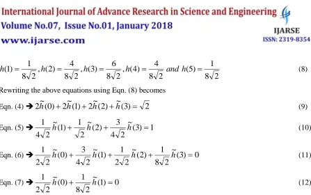
(8)
Rewriting the above equations using Eqn. (8) becomes
Eqn. (4)
2
h
~
(
0
)
2
h
~
(
1
)
2
h
~
(
2
)
h
~
(
3
)
2
(9)
Eqn. (5)
~
(
3
)
1
2
4
3
)
2
(
~
2
1
)
1
(
~
2
4
1
h
h
h
(10)
Eqn. (6)
~
(
3
)
0
2
8
1
)
2
(
~
2
2
1
)
1
(
~
2
4
3
)
0
(
~
2
2
1
h
h
h
h
(11)
Eqn. (7)
~
(
1
)
0
2
8
1
)
0
(
~
2
2
1
h
h
(12)
For a total of 4 variables, four equations are formed but in these equations only the equations (9), (10)
and (12) are independent. Hence another equation is formed below using vanishing moments. From
vanishing moments condition,
0
)
0
(
~
)
1
(
~
)
2
(
~
)
3
(
~
)
4
(
~
)
5
(
~
)
6
(
~
h
h
h
h
h
h
h
which implies
2
h
~
(
0
)
2
h
~
(
1
)
2
h
~
(
2
)
h
~
(
3
)
0
(13)
Solving (9), (10), (12) and (13) yields
.
4
2
5
)
3
(
~
32
2
5
)
2
(
~
,
8
2
3
)
1
(
~
,
32
2
3
)
0
(
~
h
h
and
h
h
By symmetry
.
32
2
3
)
6
(
~
8
2
3
)
5
(
~
,
32
2
5
)
4
(
~
h
and
h
h
Since
~
(
t
)
(
t
)
,
g
(
k
)
(
1
)
kh
~
(
N
k
1
)
. Therefore
.
32
2
3
)
5
(
8
2
3
)
4
(
,
32
2
5
)
3
(
,
4
2
5
)
2
(
,
32
2
5
)
1
(
,
8
2
3
)
0
(
,
32
2
3
)
1
(
g
g
g
g
g
and
g
g
Similarly using
g
~
(
k
)
(
1
)
kh
(
M
k
1
)
.
2
8
1
)
4
(
,
2
8
4
)
3
(
,
2
8
6
)
2
(
~
,
2
8
4
)
1
(
~
,
2
8
1
)
0
(
~
g
g
g
and
g
g
The coefficients of newly designed biorthogonal wavelet are given in the table below.
357 |
P a g e
K
-1
0
1
2
3
4
5
6
h
~
0.1326
-0.5303 0.2210 1.7678
0.2210
-0.5303 0.1326
g
~
0.0884
-0.3536 0.5303 -0.3536 0.0884
h
0.0884
0.3536 0.5303
0.3536
0.0884
g
-0.1326 -0.5303 -0.2210 1.7678 -0.2210 -0.5303 -0.1326
The above wavelet is denoted by „biors23‟ since if we take the reference as zero, the coefficients
spreads from -2 to 2 and -3 to 3. Similarly two more wavelets using spline functions with different
positioning are designed. These are „biors12‟ and „biors34‟ where the coefficients spreads from -1 to
1 and -2 to 2 and -3 to 3 and -4 to 4.
III.NEW BASIS FUNCTION BASED BIORTHOGONAL WAVELETS
The standard Spline function is defined as follows.
ki
k i
k
t
p
N
t
i
N
0
)
2
(
)
(
where
i
k
p
i k 12
1
.
Here the pi is the scaling value of dilated and translated spline function. The scaling value is directly proportional to binomial coefficients [9][10]. Hence symmetry is guaranteed. The coefficients are linearly distributed. Now a modified Spline is proposed. The new spline-like function is supposed to have symmetry but the coefficient values are modified to have more weight at center and gradually approaches standard spline function. The pi is modified and given below.
For i ≤ (k/2),
i
k
i
p
k
i 1
2
1
and
fori> (k/2),
i
k
i
k
p
k
i 1
2
1
.
358 |
P a g e
Figure 1. Coefficients of standard Spline function and proposed Spline-like functionIn Fig.1, the coefficients are given by ignoring the division by 2k-1. By using the above spline-like function with different lengths three wavelets are designed. These are denoted by „biorsl12‟, „biorsl23‟ and „biorsl34‟
respectively. The spline-like functions of length 3, 5 and 7 are utilized for „biorsl12‟, „biorsl23‟ and „biorsl34‟ respectively. The normalized coefficients of the spline-like function used for the wavelet „biorsl12‟ (k=2) are given below.
6
2
)
1
(
,
3
2
2
)
0
(
,
6
2
)
1
(
p
0
h
p
1
h
p
2
h
Similarly the coefficients for „biorsl23‟ (k=4) and „biorsl34‟ (k=6) are given below.
.
72
2
2
)
2
(
,
9
2
2
)
1
(
,
2
2
)
0
(
,
9
2
2
)
1
(
,
72
2
2
)
2
(
p
0
h
p
1
h
p
2
h
p
3
h
p
4
h
196
2
)
3
(
,
49
2
3
)
2
(
,
196
2
45
)
1
(
,
49
2
20
)
0
(
,
196
2
45
)
1
(
,
49
2
3
)
2
(
,
196
2
)
3
(
6 5 4 3 2 1 0
p
h
p
h
p
h
p
h
p
h
p
h
p
h
Using the property of double shift biorthogonality, normality, symmetry and vanishing moments
the following equations are derived for „biors1‟.
2
)
0
(
~
)
1
(
~
2
)
2
(
~
2
h
h
h
0
)
0
(
~
)
1
(
~
2
)
2
(
~
2
h
h
h
2
/
3
)
0
(
~
2
)
1
(
~
h
h
0
)
2
(
~
4
)
1
(
~
h
h
The unique solution to the above system of equations is given below.
11 1
1 2 1
1 3 3 1
1 4 6 4 1
1 5 10 10 5 1
1
1 1
1 4 1
1 6 6 1
1 8 18 8 1
1 10 30 30 10 1
359 |
P a g e
.
16
2
)
2
(
~
,
4
2
)
1
(
~
,
8
2
5
)
0
(
~
,
4
2
)
1
(
~
,
16
2
)
2
(
~
h
h
h
h
h
Similarly the coefficients for „biors1‟ and „biors2‟ are calculated and the coefficients of „coifs2‟ are
given below.
256
2
5
)
3
(
~
,
32
2
5
)
2
(
~
,
256
2
59
)
1
(
~
,
16
2
13
)
0
(
~
,
256
2
59
)
1
(
~
,
32
2
5
)
2
(
~
,
256
2
5
)
3
(
~
h
h
h
h
h
h
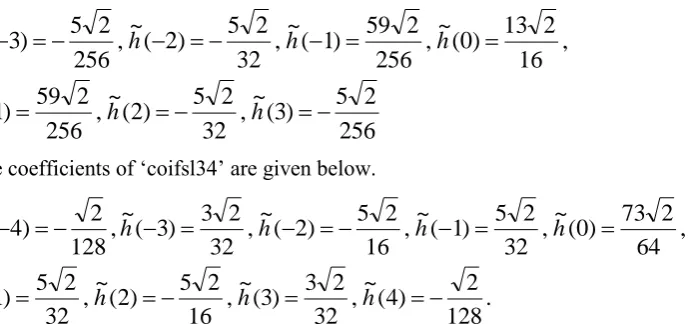
h
The coefficients of „coifsl34‟ are given below.
.
128
2
)
4
(
~
,
32
2
3
)
3
(
~
,
16
2
5
)
2
(
~
,
32
2
5
)
1
(
~
,
64
2
73
)
0
(
~
,
32
2
5
)
1
(
~
,
16
2
5
)
2
(
~
,
32
2
3
)
3
(
~
,
128
2
)
4
(
~
h
h
h
h
h
h
h
h
h
The above are scaling function coefficients at decomposition and reconstruction side. The wavelet
function coefficients are calculated from these values using expressions presented in previous
sections.
III.SIMULATION RESULTS
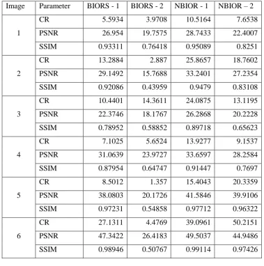
This section is concerned with the simulation results of proposed wavelets used in image compression. The image compression schemes considered are EZW [11], SPIHT [12]-[15], spatial oriented tree (STW), Wavelet difference reduction (WDR) and adaptively selected wavelet difference reduction schemes (ASWDR). The test images considered are holographic images. The simulation was carried on large number of holographic images, and results on 6 images are presented in this section. Compression ratio (CR), Peak signal to noise ratio (PSNR) and Structural similarity (SSIM) are evaluated. These values are given in Tables 2 to 6, each using different coding scheme.
Table 2. Compression results with EZW
Image
Parameter
BIORS – 1
BIORS - 2
NBIOR - 1
NBIOR – 2
1
CR
5.57
3.86
9.97
7.19
PSNR
26.95
19.76
28.74
22.40
SSIM
0.93
0.76
0.95
0.83
360 |
P a g e
SSIM
0.92
0.44
0.95
0.83
3
CR
9.47
13.45
20.71
11.07
PSNR
22.37
18.18
26.29
20.22
SSIM
0.79
0.59
0.90
0.66
4
CR
6.58
5.43
12.70
8.26
PSNR
31.06
23.97
33.66
28.26
SSIM
0.88
0.65
0.91
0.77
5
CR
7.94
1.39
13.55
17.73
PSNR
38.08
20.17
41.58
39.91
SSIM
0.97
0.55
0.98
0.96
6
CR
26.42
4.45
37.62
47.15
PSNR
47.34
26.42
49.50
44.95
SSIM
0.99
0.51
0.99
0.97
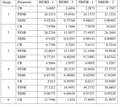
Table 3. Compression results with SPIHT
Image
Parameter
BIORS - 1
BIORS - 2
NBIOR - 1
NBIOR – 2
1
CR
3.6087
2.4404
3.2873
4.7567
PSNR
26.1213
19.0541
24.1373
21.7224
SSIM
0.92216
0.73768
0.88011
0.80482
2
CR
7.9386
1.7466
7.9539
10.643
PSNR
28.3256
15.5077
27.6953
26.2684
SSIM
0.9102
0.41597
0.88143
0.80803
3
CR
6.7296
5.2261
5.6112
8.3216
PSNR
22.0015
15.1597
21.1496
19.8948
SSIM
0.77251
0.40269
0.71882
0.63342
4
CR
4.5664
1.9557
4.0095
5.5267
PSNR
30.502
20.2151
29.4054
27.5773
SSIM
0.87192
0.48083
0.82902
0.74209
5
CR
5.013
0.49591
8.6217
10.9985
PSNR
37.1212
16.9451
40.3732
38.6803
SSIM
0.96775
0.40436
0.97251
0.95226
361 |
P a g e
PSNR
41.5796
23.7292
45.6326
43.0904
SSIM
0.96395
0.39073
0.97201
0.94831
Table 4. Compression results with STW
Image
Parameter
BIORS - 1
BIORS - 2
NBIOR - 1
NBIOR – 2
1
CR
5.1325
3.539
4.5776
6.7078
PSNR
27.019
19.7979
25.0451
22.4944
SSIM
0.93389
0.76529
0.89598
0.82735
2
CR
11.8474
2.5152
11.9654
16.0436
PSNR
29.2839
15.7668
28.8566
27.5245
SSIM
0.92252
0.43953
0.89834
0.83928
3
CR
9.785
7.7449
7.9707
11.6272
PSNR
22.4244
15.4869
21.6035
20.2766
SSIM
0.79177
0.4317
0.74118
0.65956
4
CR
6.4997
2.8392
5.5842
7.7993
PSNR
31.1967
20.6166
30.3031
28.6499
SSIM
0.8825
0.51031
0.84624
0.77924
5
CR
7.4443
0.68715
13.3372
17.249
PSNR
38.4664
17.1371
43.1523
42.296
SSIM
0.97358
0.41315
0.98101
0.97146
6
CR
17.3925
2.3371
26.6846
33.9111
PSNR
43.9615
24.0129
50.1329
48.9213
SSIM
0.97599
0.42525
0.98848
0.98061
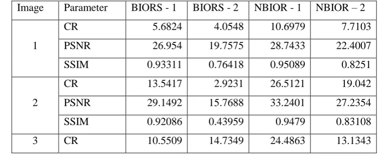
Table 5. Compression results with WDR
Image
Parameter
BIORS - 1
BIORS - 2
NBIOR - 1
NBIOR – 2
1
CR
5.6824
4.0548
10.6979
7.7103
PSNR
26.954
19.7575
28.7433
22.4007
SSIM
0.93311
0.76418
0.95089
0.8251
2
CR
13.5417
2.9231
26.5121
19.042
PSNR
29.1492
15.7688
33.2401
27.2354
SSIM
0.92086
0.43959
0.9479
0.83108
362 |
P a g e
PSNR
22.3746
18.1767
26.2868
20.2228
SSIM
0.78952
0.58852
0.89718
0.65623
4
CR
7.1452
5.7958
14.0335
9.1283
PSNR
31.0639
23.9727
33.6597
28.2584
SSIM
0.87954
0.64747
0.91447
0.7697
5
CR
9.0083
1.413
16.2094
21.4671
PSNR
38.0803
20.1726
41.5846
39.9106
SSIM
0.97231
0.54858
0.97712
0.96322
6
CR
28.3427
4.6178
40.7277
52.3137
PSNR
47.3422
26.4183
49.5037
44.9486
SSIM
0.98946
0.50767
0.99114
0.97426
Table 6. Compression results with ASWDR
Image
Parameter
BIORS - 1
BIORS - 2
NBIOR - 1
NBIOR – 2
1
CR
5.5934
3.9708
10.5164
7.6538
PSNR
26.954
19.7575
28.7433
22.4007
SSIM
0.93311
0.76418
0.95089
0.8251
2
CR
13.2884
2.887
25.8657
18.7602
PSNR
29.1492
15.7688
33.2401
27.2354
SSIM
0.92086
0.43959
0.9479
0.83108
3
CR
10.4401
14.3611
24.0875
13.1195
PSNR
22.3746
18.1767
26.2868
20.2228
SSIM
0.78952
0.58852
0.89718
0.65623
4
CR
7.1025
5.6524
13.9277
9.1537
PSNR
31.0639
23.9727
33.6597
28.2584
SSIM
0.87954
0.64747
0.91447
0.7697
5
CR
8.5012
1.357
15.4043
20.3359
PSNR
38.0803
20.1726
41.5846
39.9106
SSIM
0.97231
0.54858
0.97712
0.96322
6
CR
27.1311
4.4769
39.0961
50.2151
PSNR
47.3422
26.4183
49.5037
44.9486
363 |
P a g e
IV.CONCLUSIONS
In this paper, new biorthogonal wavelets are proposed. The newly designed wavelets are used for image compression. Five different wavelet based image compression techniques are considered. They are EZW, SPIHT, STW, WDR, and ASWDR. Simulations are performed on Holographic images. The main observation from the simulation results is that the compression ratio using proposed wavelets is extremely high in comparison with that of in existing wavelets. In most of the cases the compression ratio using proposed wavelets is more than twice that of the existing wavelets. In addition to achieving high compression ratio a tolerable PSNR was maintain.The spline function when changed by considering a criterion and also when the input images classified based on their characteristics, a more generalized and optimum mother wavelet function can be devised with the analysis present in this paper.
REFERENCES
[1] Ronald A. DeVore, “Adaptive Wavelet Bases for Image Compression”, A K Peters Wavelets, Images and
Surface Fitting, pp. 197-219, 1994.
[2] Yan Zhuang, John S. Baras, “Image compression using optimal wavelet basis”, Proc. of SPIE, 17-21 April
1995.
[3] Michael G. Strintzis, “Optimal Biorthongoal Wavelet Bases for Signal Decomposition”, IEEE Transactions on Signal Processing, vol. 44, no. 6, pp. 1406-1417, June 1996.
[4] Aleksandra Mojsilovic, Miodrag V. Popovic and Dejan M. Rackov, “On the Selection of an Optimal Wavelet Basis for Texture Characterization”, IEEE Transactions on Image Processing, vol. 9, no. 12, pp. 2043-2050,
Dec 2000.
[5] Nasir M. Rajpoot, Roland G. Wilson, Francois G. Meyer, Ronald R. Coifman, “Adaptive Wavelet Packet Basis Selection for Zerotree Image Coding”, IEEE Transactions on Image Processing, vol. 12, no. 12, Dec
2003.
[6] M. K. Mandal, S. Panchanathan and T. Aboulnasr, “Choice of Wavelets for Image Compression”, Springer
Lecture Notes in Computer Science, vol. 1133, pp. 239-249, 2005.
[7] G. K. Kharate, V. H. Patil and N. L. Bhale, “Selection of mother wavelet for image compression on basis of
image”, Journal of Multimedia, vol. 2, no. 6, November 2007.
[8] Maria Rehman, Imran Touqir, WajihaBatool, “Selection of optimal wavelet bases for image compression using SPIHT algorithm”, Proc. SPIE 9445, Seventh International Conference on Machine Vision (ICMV
2014), vol. 9445, Feb 2015.
[9] Noor Kamal Al-Qazzaz, Sawal Hamid Bin Mohd Ali, SitiAnom Ahmad, MohdShabiul Islam and Javier Escudero, “Selection of Mother Wavelet Functions for Multi-Channel EEG Signal Analysis during a Working Memory Task”, Sensors, 15, pp. 29015-29035, 2015.
[10] GirishaGarg, “A signal invariant wavelet function selection algorithm”, Springer Medical & Biological
364 |
P a g e
[11] Shapiro J.M. (1993), "Embedded image coding using zerotrees of wavelet coefficients",P IEEE Trans. Signal Proc., Vol. 41, No. 12, pp. 3445–3462.
[12] Said A., W.A. Pearlman (1996), "A new, fast, and efficient image codec based on set partitioning in hierarchical trees," IEEE Trans. on Circuits and Systems for Video Technology, Vol. 6, No. 3, pp. 243–250.
[13] Jaya Krishna Sunkara, PurnimaKuruma, Ravi Sankaraiah Y, “Image Compression Using HandDesigned and
Lifting Based Wavelet Transforms”, International Journal ofElectronics Communications and Computer Technology (e-ISSN: 2249-7838, IF: 1.2456), Vol. 2 (4),2012.
[14] Jaya Krishna Sunkara, E Navaneethasagari, D Pradeep, E Naga Chaithanya, D Pavani, D V SaiSudheer,“ANewVideoCompressionMethodusingDCT/DWTandSPIHTbasedonAccordionRepresentation”,
I.J. Image, Graphics and Signal Processing (e-ISSN: 2074-9082, p-ISSN:2074-9074,IF: 0.11), pp. 28-34, May2012.
[15] JayaKrishnaSunkara,KurumaPurnima,ENavaneethaSagariandLRamaSubbareddy,“ANewAccordion Based Video Compression Method”, i-manager‟s Journal on Electronics Engineering(e-ISSN: 2249-0760, p-ISSN:
2229-7286), Vol. 1, No. 4, pp. 14-21, June - August2011.
Author‟s Profile
N. Hyndavi, received her Bachelors in Technology in Electronics and Communication
Engineering from Priyadarshini College of Engineering, Sullurpet affiliated to JNTUA, Ananthapuramu in 2015. Currently she pursuing Masters in Technology in Digital Electronics and Communication Systems in Gokula Krishna College of Engineering, Sullurpet. Her research interests include Signal and Image Processing and wavelet analysis.
T.Aruna, received her B.Tech degree in ECE from Audisankara College of Engineering and