Evaluate Hourly based Load Forecasting
using NARX Neural Network in MATLAB
Environment
Anil Patel1, Albert John Varghese2
M. E Scholar, Department of ELE, Rungta College of Engineering and Technology, Bhilai, Chhattisgarh, India1
Assistant Professor, Department of ELE, Rungta College of Engineering and Technology, Bhilai, Chhattisgarh, India2
ABSTRACT: In this paper, neural network based time series forecasting of load has been done. A nonlinear autoregressive network with exogenous input (NARX) has opted for the proposed model of time series forecasting. Load data has taken from a boys hostel Bhilai, Chhattisgarh. This paper proposed that an hourly based prediction model of load data, in which previous data of load has been used for predicting the future values of load data. Neural network were prepared with some previous data, some of which were used in data training and some data were used in simulation. Setup division for data training, validation and testing should be 50/25/25. Levenberg-Marquardt (LM) algorithm has been used for training purpose. Comparison of predicted load data and measured data has been also performed. The entire implementation of proposed model has been done in MATLAB environment.
KEYWORDS:NARX, time series forecasting, neural network, predict, MATLAB.
I.INTRODUCTION
Electricity is presumed to be the basis for the progress of civilization, so it is of great importance as a tool for the technological advancement and economic development of the society [1]. To supply sufficient power to the customer, demand for their load should be known. This evaluation process of future demand of load is called ‘Load forecast’. The prediction of the load is the launch of electric load, which will require the use of the previous power in the field required by a specific geographical area. Loading, which helps in making important decisions related to the system, therefore, the load forecasting is very important for successful effective and efficient operation of any energy system [2].
II. NARX NEURAL NETWORK
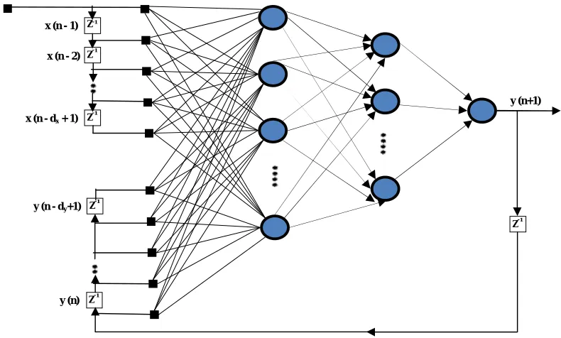
NARX network is a dynamic neural structure that is initially used for input output modeling of non-linear dynamic system. When applied on the prediction of the time series, the NARX network is designed as the Feed Forward Time Delay Neural Network (TDNN), meaning that without its feedback loop of delay output, its predicted performance has been reduced to a great extent [3].
The dynamic equation of NARX neural network is shown in bellow equation (1).
y(n + 1) = f[y(n), y(n−1), … … . , y n−d + 1 ; u(n), u(n−1), … … . , u(n−d + 1)](1)
Where,
du≥ 1, dy≥ 1, and du ≤ dyis the input memory and output memory order. The following figure-1 shows the NARX
network [3].
The following figure 2 indicates the architecture of neural network based NARX Model, which clearly describe the estimated values of NARX Model is depend on previous input and previous output.
III.LITERATURE REVIEW
Cristhian Moreno-Chaparro et.al, proposed a monthly, power prediction method for the Columbia National Interconnected System in which the original series data was thus used in a non-linear behaviour, a neural non- linear autoregressive (NAR) model. Here prediction was received by adding estimates with the predicted tendency to be combined with the residual chain obtained by the adding pre-processing components.
Isaac Samuel et.al, presented a method and comparative study between time series prediction and artificial neural network method, where real time data of load for Covenant University was used. Comparison performs within the exponential smoothing andmoving average of time-series method, and the Artificial Neural Network (ANN) models, where ANN method was best method for prediction when compared the results in terms of error calculation with amean absolutedeviation(MAD).
NARX Model Output of Model Input of Model
Z-1
Z-1
Z-1
Z-1 Z-1
Z-1
y (n+1)
y (n) y (n - dy+1) x (n)
x (n - 1)
x (n - 2)
x (n - dx + 1)
Figure 1- NARX neural network with du delayed inputs and dy delayed outputs
Jose Maria P. Junior et.al, proposed that the architecture ofNARX neural network which in easily applied in multi-step ahead forward prediction of time-series real world data. The proposed method used two real-time data sets. Nameof the method wasthe variable bit rate (VBR) video tra c and chaotic laser time series, which are used in proposed model.
Shapna Muralidharan et.al, developed a Short Term Load Prediction model usingNon-LinearAutoregressivewith the exogenousinputs(NARX) method in ANN and estimated the day-forwarded electricity, which need for a year per hour granularity. Proposed model need to takethe seasonal variables the temperatures as exogenous inputs. The Short Term Load Prediction model used many training algorithms for simulate the data and 2% of least error rate is obtained, which can ensure better predicting solution.
Md. Umar Hashmi et.al, proposed themethod, which required low real time inputs like weather information. The load consumption real time data (in MW) for two and ahalf year of GEB (Goa Electricity Board) of Goa, India is used in the future load demand estimation. The results received from the proposed model proudly estimates the future values of load data with mean square error (MSE) ≤ 1.67% and mean absolute deviation ≤ 3.6%, which was suitable of forecast to proposed technique.
IV. METHODOLOGY
In this paper, proposed model is implemented by using neural network based NARX model in MATLAB environment. For this, load data has been collected from a boy’s hostel, Bhilai, Chhattisgarh on 07/03/2017. The entire data has been collected on hourly basis of 24 hours, which is shown in following table-1. Only few data will be used in model, in which time is set into input series and measured load data is set into target series. Rest of the data will used in simulates the data for prediction purpose. Further comparison between predicted data and measured data has been performed in this paper.
Time (hour) Measured load data (KWH)
1 2.1
2 1.9
3 1.8
4 1.8
5 2.0
6 2.3
7 2.5
8 3
9 2.8
10 2.6
11 2.1
12 1.9
13 1.8
14 1.9
15 1.8
16 2.1
17 2.3
18 2.3
19 2.2
20 2.5
21 2.3
22 2.1
23 1.9
24 2.0
Parameters which had used in programming of proposed model are described in following table-2.
Parameters Values
Number of previous data used in model 8
Number of input delays 6
Number of feedback delays 6
Number of neurons in hidden layer 28
% Division of used data for training/validation/testing 50 /25/25 Number of time horizon for forecasting (N) 15 Table 2 – Parameters used in MATLAB Programming for proposed model.
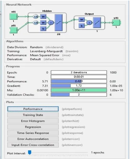
Used measured data in model had trained by Levenberg-Marquardt (LM) algorithm. It is nothing but just an adjustment of bias values according to the target series data. In LM algorithm data had divided into 50 %, 25% and 25% for training, validating and testing respectively. In figure-3, shows the training of data, where number of epoch, time of training processand performance are described.
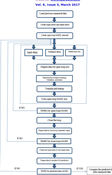
In figure-4, the entire steps of programming the proposed model in MATLAB environment are described by using flowchart, which is very easy and convenient for understanding the whole model. In programing of model, NMSE (normalised mean square error) values should be less than 0.005 for open loop, close loop and predicted output. The neural network was trained by using different number of parameter till NMSE ≤ 0.005 was obtained. Further rest of the measured data was simulated for obtaining predicted data. Mathematical formula of NMSE is shown in equation (2).
Create input series and target series Load previous measured data
Create open loop NARX network
Input delay Feedback delay Hidden layer size
Prepare data for open loop n/w
Training and testing
NMSE for open loop<<0.005 View open loop NARX n/w
Close the loop
Prepare data for close loop & generate output
NMSE for close loop<<0.005
Create new input series & new target series
Prepare data & simulate it for prediction
NMSE for predicted data<<0.005
Setup division of data for training, Validation, and testing
If NO
If NO
If NO If YES Compare the predicted data
with measured data
In figure-5 & 6, shows the open loop and close loop of NARX Network respectively, where number of delays and size of hidden layer are shown in great extent.
V.RESULTS AND DISCUSSION
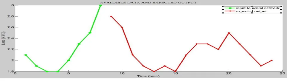
As seen in figure-7, curve in green colour shows behaviour of available data which is used in NARX Model as target series and curve in red colour shows the expected output load data, which has to be predicted. The available data which are using in proposed model which give some predicted data that must be very close to expected output load data.
After run the proposed model in MATLAB environment, it gives some predicted data as shown in figure-8. As seen in figure-8, curve in blue colour shows the behaviour of predicted data.
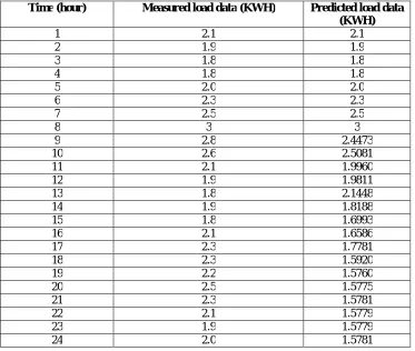
Figure-9 shows the comparison between expected load data and predicted load data. This curve describes how close the predicted data, from measured data. All the predicted values of load for different time horizon are shown in table-3.
Figure 5 – Open loop NARX Network. Figure 6 – Close loop NARX Network.
Figure 7 – Available data for NARX Model and expected measured data
After comparison between expected output and predicted output data, we can evaluate that proposed model can forecast the few time horizon errorless and other time horizons have large error. Therefore further modification required in proposed model. The following table-3 shows the comparison between measured load data and predicted load data.
Time (hour) Measured load data (KWH) Predicted load data (KWH)
1 2.1 2.1
2 1.9 1.9
3 1.8 1.8
4 1.8 1.8
5 2.0 2.0
6 2.3 2.3
7 2.5 2.5
8 3 3
9 2.8 2.4473
10 2.6 2.5081
11 2.1 1.9960
12 1.9 1.9811
13 1.8 2.1448
14 1.9 1.8188
15 1.8 1.6993
16 2.1 1.6586
17 2.3 1.7781
18 2.3 1.5920
19 2.2 1.5760
20 2.5 1.5775
21 2.3 1.5781
22 2.1 1.5779
23 1.9 1.5779
24 2.0 1.5781
Table 3- Comparison of measured load data and predicted load data
VI. CONCLUSION
In this paper, hourly based load forecasting by using NARX neural network has been done in MATLAB environment. All the parameters used in proposed model can be evaluated analytically by training process repetition until NMSE ≤
0.005. The entire steps for time series forecasting like data collection, open loop creation, close loop creation, and further simulate the data for prediction has been successfully performed in this paper. The comparison of predicted load data and actual measured data are also performed.
REFERENCES
[1]. Cristhian Moreno-Chaparro, Jeison Salcedo-Lagos, Edwin Rivas, and Alvaro Orjuela Canon, “A Method for the Monthly Electricity Demand
Forecasting in Colombia based on Wavelet Analysis and a Nonlinear Autoregressive Model”, INGENIERÍA ,Vol. 16, Issue No. 2, pp. 94-106, 2011.
[2]. Isaac Samuel, Tolulope Ojewola, Ayokunle Awelewa, and Peter Amaize, “Short-Term Load Forecasting Using The Time Series And Artificial
Neural Network Methods”, IOSR Journal of Electrical and Electronics Engineering (IOSR-JEEE), e-ISSN: 2278-1676, p-ISSN: 2320-3331, Vol. 11, Issue. 1, pp. 72-81, 2016.
[3]. Jose Maria P. Junior and Guilherme A. Barreto, “Long-Term Time Series Prediction with the NARX Network: An Empirical Evaluation”
Elsevier Science, page 1 & 6, 2007.
[4]. Abdullateef Ayodele Isqeel, Tijani Bayo Ismaeel, and Salami Momoh-Jimoh Eyiomika, “Consumer Load Prediction Based on NARX for
Electricity Theft Detection”,IEEE-2016 International Conference on Computer & Communication Engineering, DOI 10.1109/ICCCE.2016.70, pp.294-299, 2016.
[5]. Yang Chunshan, and Li Xiaofeng, “Study and Application of Data Mining and NARX Neural Networks in Load Forecasting”, ICCSNT 2015,
IEEE- 4th International Conference on Computer Science and Network Technology (ICCSNT), pp.360-364, 2015.
[6]. Luciano Carli M. de Andrade, Mario Oleskovicz, and Ricardo Augusto Souza Fernandes, “Very Short-Term Load Forecasting Based on NARX
Recurrent Neural Networks”, IEEE, 2014.
[7]. SUCI DWIJAYANTI, “SHORT TERM LOAD FORECASTING USING A NEURAL NETWORK BASED TIME SERIES APPROACH”,
Bachelor of Science in Electrical Engineering Sriwijaya University Palembang, Indonesia , pp.1-117, 2006.
[8]. Jaime Buitrago, and Shihab Asfour, “Short-Term Forecasting of Electric Loads Using Nonlinear Autoregressive Artificial Neural Networks
with Exogenous Vector Inputs”, Energies, vol.10, issue.40, 2017.
[9]. Md. Umar Hashmi, Varun Arora, and Jayesh G. Priolkar,” Hourly electric load forecasting using Nonlinear AutoRegressive with eXogenous
(NARX) based neural network for the state of Goa, India”, IEEE- International Conference on Industrial Instrumentation and Control (ICIC), pp.1418-1423 May 28-30,2015
[10].Vahid Mansouri, and Mohammad E. Akbari, “Neural Networks in Electric Load Forecasting: A Comprehensive Survey”, IEEE- Journal of
Artificial Intelligence in Electrical Engineering, Vol. 3, No. 10, pp.37-50, 2014.
[11].Shapna Muralidharan, Abhishek Roy, and Navrati Saxena, “Stochastic Hourly Load Forecasting for Smart Grids in Korea Using NARX
Model”, IEEE, pp.167-172, 2014.
[12].www.sci-hub.cc , 13/03/2017.
[13].www.mathworks.com , 26/02/2017.