Article 1
Improve Building Façades in Open Lidar Data using
2Ground Imagery
3Shenman Zhang 1,*, Pengjie Tao 1 4
1 School of Remote Sensing and Information Engineering, Wuhan University, 430079, Wuhan, China 5
* Correspondence: [email protected] 6
7
Abstract: Recent advances in open data initiatives allow us to free access to a vast amount of open 8
LiDAR data in many cities. However, most of these open LiDAR data over cities are acquired by 9
airborne scanning, where the points on façades are sparse or even completely missing due to the 10
viewpoint and object occlusions in the urban environment. Integrating other sources of data, such 11
as ground images, to complete the missing parts is an effective and practical solution. This paper 12
presents an approach for improving open LiDAR data coverage on building façades by using point 13
cloud generated from ground images. A coarse-to-fine strategy is proposed to fuse these two 14
different sources of data. Firstly, the façade point cloud generated from terrestrial images is initially 15
geolocated by matching the SFM camera positions to their GPS meta-information. Next, an 16
improved Coherent Point Drift algorithm with normal consistency is proposed to accurately align 17
building façades to open LiDAR data. The significance of the work resides in the use of 2D 18
overlapping points on the outline of buildings instead of limited 3D overlap between the two point 19
clouds and the achievement to a reliable and precise registration under possible incomplete 20
coverage and ambiguous correspondence. Experiments show that the proposed approach can 21
significantly improve the façades details of buildings in open LiDAR data and improving 22
registration accuracy from up to 10 meters to less than half a meter compared to classic registration 23
methods. 24
Keywords: Open LiDAR; Terrestrial Images; Building Reconstruction; Point Cloud Registration 25
26
1. Introduction 27
In recent years, there has been a significant push from the open data initiatives in many North 28
American cities [1–3] or the large projects such as Infrastructure for Spatial Information in the 29
European Community (INSPIRE) [4,5] proposed by European Commissions to provide vast amounts 30
of open datasets that also include open LiDAR data [6,7]. Nowadays, open LiDAR data covering most 31
parts of Europe and North America are already available for the public. Due to the free access to these 32
open LiDAR data, new avenues of research for students, researchers, and other LiDAR data user 33
community have been opened [8–10]. However, these open LiDAR data are often sparse and 34
incomplete, or even entirely void on the façades due to the viewpoint and occlusions in the urban 35
environment. This problem makes it difficult to achieve fine building reconstruction with high levels 36
of detail (LoD) [11]. 37
Recently, ground imagery capture devices such as off-the-shelf digital cameras, smartphones 38
with GPS and digital compass have become ever prevalent. They allow us to acquire a number of 39
high-resolution images of the building façade through crowd-sourcing at low cost. Additionally, the 40
state-of-the-art Structure-from-Motion (SfM) and Multi-View Stereo (MVS) reconstruction 41
techniques [12–16] allow us to process these ground images so as to recover façades information in 42
fine detail and precision. Considering that ground images are complementary to open LiDAR data 43
in terms of façade details, fusing façade point cloud generated from ground images into open LiDAR 44
data is a promising way to improve open LiDAR data on the details of façade. 45
Various researches have been studied on the fusion of multiple sources of data to reconstruct 46
buildings with rooftops and façades information. Boulaassal et al. [17] combined airborne LiDAR 47
scanning (ALS), terrestrial LiDAR scanning (TLS) and vehicle LiDAR scanning (VLS) data to produce 48
reliable 3D building models, however, the high costs of using several kinds of laser scanners limited 49
the applications of this technique. Besides, the success of this combination relied on a controlled and 50
corrected geo-referencing of GPS before processing. Shan et al. [18] addressed this problem using a 51
viewpoint-dependent matching method so that the aerial and the ground images could be accurately 52
matched to generate high-quality multi-view stereo models. However, this depends on the quality of 53
ground imagery and its similar appearance with the aerial images. Wang et al. [19] proposed a system 54
for aligning 3D SfM point clouds produced from Internet imagery to existing Google Earth 3D models 55
and Google Street View photos. Their method relied on the quality of Google Earth 3D models which 56
often is not very credible and may vary in different cities. 57
Essentially, the fusion of façade point cloud and open LiDAR data is a process of point set 58
registration that maps one point set to the other according to their correspondence. Point set 59
registration is a crucial step in many computer vision and photogrammetry tasks including stereo 60
matching [20], medical imaging [21], heritage reconstruction [22], shape retrieval [23] and industrial 61
applications [24]. Iterative Closest Point (ICP) [25] is the most widely used and classic point sets 62
registration algorithm due to its simplicity and low computational complexity. It iteratively assigns 63
correspondence based on the closest distance criterion and finds the least-squares transformation 64
between the pair of point sets until a local minimum is reached. A major drawback of ICP algorithm 65
is that it demands an accurate initial guess of the correspondence between two point sets. Otherwise, 66
it may fall into a local minimum or even be non-convergent. A lot of ICP-based variants have been 67
proposed to address the weaknesses [26–30]. Myronenko et al. proposed a probabilistic-based point 68
set registration algorithm [31] which is called Coherent Point Drift (CPD). CPD considers the 69
alignment of a pair of point sets as a probability density estimation problem where one point set 70
represents the Gaussian Mixture Model (GMM) centroids, and the other one represents the data 71
points. The rigid transformation that aligns GMM centroids to data points is obtained by maximizing 72
the GMM posterior probability for data points at the optimum. The CPD algorithm, which exhibits a 73
linear computational complexity, outperforms most state-of-the-art algorithms and achieves 74
promising results with respect to conditions of noise, outliers, and missing points. 75
Nonetheless, the alignment between façade point cloud and open LiDAR data remains a 76
problem because of (1) inevitable noise points in facade point cloud, including noise points from SfM 77
and MVS procedure and noise points of other ground objects such as trees, lamp-posts, and passers-78
by; (2) limited overlaps between the two point clouds; (3) their large density difference; and (4) their 79
large initial offset. All these issues lead to a challenge to traditional point sets registration algorithms. 80
This paper presents a novel method for improving open LiDAR data on the building façade 81
using the façade point cloud generated from ground images. Firstly, to reduce the significant 82
differences in rotation, scale, and translation between the two kinds of point cloud, we achieve initial 83
geolocation of façade point cloud by matching the SfM camera positions to their GPS imaging meta-84
data. Then, a modified CPD algorithm with normal consistency is proposed to achieve precise 85
registration by making full use of similarity on 2D outlines of buildings. The significance of the work 86
resides in the best use of the most likely overlap between the two point clouds and the achievement 87
to a reliable and precise registration under possible incomplete coverage and ambiguous 88
90
Figure 1. The overview of the proposed method. 91
The remainder of this paper is structured as follows. In section 2, we describe our approach for 92
aligning façade point cloud generated from ground images to open LiDAR data. Section 3 presents 93
the test results and discusses its performance. Finally, we conclude in section 4. 94
2. Methodology 95
Given ground image set {𝑰𝒊|𝑖 = 1,2, … 𝐺}, COLMAP [32], a general-purpose
Structure-from-96
Motion (SfM) and Multi-View Stereo (MVS) pipeline, is used to generate the facade point cloud 𝓜 97
and camera positions {𝑪𝒊 |𝑖 = 1, 2 , … 𝐺} in SfM local coordinate system. Additionally, the GPS 98
meta-information {𝑪𝒊 |𝑖 = 1, 2 , … 𝐺} of these images are extracted from the EXIF information of
99
{𝑰𝒊}. Corresponding to the capture area of {𝑰𝒊}, the open LiDAR data 𝓟 with precise geographic 100
coordinates are also given. 101
𝓟 , 𝓜 , {𝑪𝒊 } and {𝑪𝒊 } are taken as the input. The facade point cloud 𝓜 accurately
102
aligned to the corresponding open LiDAR data 𝓟 is the ultimate output. The whole alignment 103
process is performed in a two-step strategy: First, an initial georegistration is performed by 104
approximately transforming 𝓜 into the geo-referenced coordinate system according to a 105
matching between {𝑪𝒊 } and {𝑪𝒊 }. Second, a modified Coherent Point Drift algorithm with 106
normal consistency (NC-CPD) is proposed to accurately align the façade point cloud to open LiDAR 107
data. 108
2.1. Initial Georegistration 109
Since the alignment between facade point cloud 𝓜 in the local coordinate system and open 110
LiDAR data 𝓟 in geo-referenced coordinate system features large scale, translation and rotation 111
differences, a georegistration is performed to approximately transform 𝓜 to geo-referenced 112
coordinate to reduce these differences at first. 113
Levelling the Facade Point Cloud. As a first step in the initial georegistration, we level the facade 114
point cloud 𝓜 to the upright direction (the opposite of the gravity vector) by estimating the 115
upright vector 𝑫 on the assumption that 𝑫 should be perpendicular to the normal vectors of 116
all façade points in 𝓜 . An initial upright vector 𝑫 is calculated by fitting a plane to the camera 117
positions {𝑪𝒊 } obtained in SfM process on the assumption that images are captured approximately
118
on one plane. Then, candidate façade points {𝑝 } whose normal vectors 𝑵 are approximately 119
perpendicular to 𝑫 , in other words |𝑵 𝑫 | < 0.3, are extracted. After that, a RANSAC-based 120
approach is applied to refine the accurate upright vector 𝑫 by iteratively selecting two points from 121
facade point cloud 𝓜 is acquired by rotating 𝓜 to make the Z-axis in its coordinate system 123
parallel to 𝑫 . 124
Geolocation of Leveling Facade Point Cloud using GPS meta-data. Since the SfM procedure has 125
recovered the facade point cloud as well as cameras (images) shooting positions in the same local 126
coordinate system, the problem of geolocating the facade point cloud can be converted into the 127
problem of locating the SfM camera positions to the geo-referenced coordinate system, as shown in 128
Figure 2. Due to GPS positioning features a dramatic accuracy difference between horizontal and 129
altitude direction, a planar transformation and a vertical translation is calculated respectively. 130
(a) (b) (c)
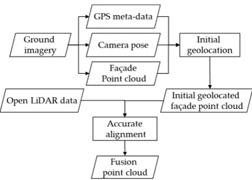
Figure 2. The overview of the initial georegistration process. Camera positions calculated in SfM (Red 131
points in Figure. a) and camera GPS meta information (Green points in Figure. b) are matched using 132
a RANSAC-based similarity transformation. Simultaneously, the facade point cloud (textured points 133
in Figure. a) is aligned to point cloud of building from the open LiDAR data (blue points in Figure. b) 134
by using the calculated similarity transformation parameters. The alignment result is shown in Figure. 135
c. 136
A RANSAC-like 2D similarity transformation is estimated between the camera positions’ x-y 137
coordinates in local SfM coordinate and their corresponding longitude and latitude of GPS: Given 138
the local coordinates {𝑪𝒊 } and the geo-referenced coordinates {𝑪𝒊 } of the ground cameras, 139
the minimal subset (size 3) of the ground cameras for point sets registration is selected from {𝑪𝒊 } 140
and {𝑪𝒊 } at random. Then, the 2D–2D similarity transformation is estimated using the least-141
squares solver, and the similarity transformation parameters are calculated. The inlier set of the 142
estimated transformation is obtained with the inlier threshold ε. This process is repeated to obtain 143
the maximal consensus set, which has the maximal number of inliers. Finally, the similarity 144
transformation {𝑠𝒄𝒂, 𝑹𝒄𝒂, 𝑻𝒄𝒂} for geolocating the cameras (images) as well as the facade point cloud 145
into the geo-referenced coordinate system is estimated with this maximal consensus set using the 146
least-square method again. This procedure is formulated in Equation2. 147
𝑪𝒊𝑮𝑷𝑺 𝟐𝑫= 𝑠𝒄𝒂 𝑹𝒄𝒂𝑪𝒊𝒍𝒐𝒄 𝟐𝑫+ 𝑻𝒄𝒂, 𝑖 = 1, . . . 𝑁
𝓣(𝑠𝒄𝒂, 𝑹𝒄𝒂, 𝑻𝒄𝒂) ← 𝑅𝐴𝑁𝑆𝐴𝐶(𝑠𝒄𝒂, 𝑹𝒄𝒂, 𝑻𝒄𝒂) (1)
Then, a vertical translation 𝑻𝒄𝒂 is calculated by matching the mean value of z coordinate in 148
{𝑪𝒊 } and mean value of altitude in {𝑪𝒊 }. Finally, apply transformation {𝑠𝒄𝒂, 𝑹𝒄𝒂, 𝑻𝒄𝒂} to 149
(x, y) coordinate of 𝓜 and transformation {𝑠𝒄𝒂, 𝑻𝒄𝒂} to z coordinate of 𝓜 , initial geolocated 150
Scale, translation and rotation differences are greatly relieved after initial alignment as described 152
above, although there are meter-level [33] alignment errors between the initial geolocated facade 153
point cloud 𝓜 and the open LiDAR point cloud 𝓟 due to the GPS location uncertainties. 154
2.2. Extended Coherent Point Drift with Normal Consistency (NC-CPD) 155
To further reduce the initial alignment errors, accurate alignment is necessary for obtaining 156
reliable and precise correspondences between 𝓜 and 𝓟 . Because of inevitable noise points in 157
facade point cloud, including noise points generated in the SfM and MVS procedure and noise points 158
of other ground object such as trees, lamp-posts and passers-by, an improved CPD algorithm with 159
normal consistency is used to register the two point clouds with noise and structure ambiguities. 160
Coherent Drift Algorithm. This algorithm was first introduced in [31] for considering the alignment 161
of two point sets as a probability density estimation. Given two D-dimensional point sets 𝑿 × = 162
(𝒙 , … , 𝒙 ) and 𝒀 × = (𝒚 , … , 𝒚 ), CPD method considers the alignment of the two point sets as a 163
probability density estimation problem where one point set represents the GMM centroids (𝒀 × ) 164
and the other one represents the data points (𝑿 × ). The rigid transformation 𝓣(𝑹 , 𝑠, 𝑻) that aligns 165
GMM centroids 𝒀 × to data points 𝑿 × are obtained by maximizing the GMM posterior 166
probability for the data point 𝑿 × at the optimum. The GMM probability density function of CPD 167
can be written as Equation 2: 168
𝑝(𝒙) = 𝑃(𝑚)𝑝(𝒙|𝑚) (2)
where 𝑝(𝒙|𝑚) =( ) / 𝑒𝑥𝑝 ‖ ‖ and a uniform distribution 𝑝(𝒙|𝑀 + 1) = 1 𝑁⁄ is used to 169
account for outliers and the weight of it is donated as 𝜔 (0 ≤ 𝜔 ≤ 1). 𝑃(𝑚) = 1 𝑀⁄ for all GMM 170
components. Then, the mixture model takes the form: 171
𝑝(𝒙) = 𝜔1
𝑁+ (1 − 𝜔)
1
𝑀 𝑝(𝒙|𝑚) (3)
GMM centroids locations are re-parametrised by rigid transformation parameters (𝑹, 𝑠, 𝒕). We can 172
estimate them by maximizing the negative likelihood function: 173
𝐸(𝑹, 𝑠, 𝒕, 𝜎 ) = −𝑙𝑜𝑔 𝑝(𝒙 ) = − 𝑙𝑜𝑔 𝑃(𝑚)𝑝(𝒙 |𝑚) (4)
The correspondence probability is defined between two points 𝐲 and 𝐱 as the posterior 174
probability of the GMM centroids given the data points: 𝑃(𝑚|𝒙 ) = 𝑃(𝑚)𝑝(𝒙 |𝑚)/𝑝(𝒙 ) 175
The estimation of parameters (𝑹, 𝑠, 𝒕, 𝜎 ) can use the Expectation Maximization (EM) algorithm. 176
The first step (E step) : predicts the value of parameters based on previous values (𝑹 , 𝑠, 𝑻) and 177
then Bayes’ theory is used to calculate a posteriori probability distributions as the following equation: 178
𝑝 = 𝑃 (𝑚|𝒙 ) = 𝑝(𝒙 |𝑚)
∑ 𝑝(𝒙 |𝑚) + (2𝜋𝜎 ) / 𝜔
1 − 𝜔𝑀𝑁 (5)
The second step (M step): obtain new parameters by minimising negative logarithm likelihood 179
function of Equation 4. The EM algorithm proceeds by alternating between E and M-steps until 180
convergence. After ignoring the constants independent of (𝑹, 𝑠, 𝒕, 𝜎 ), it can be written as: 181
𝑄(𝑹, 𝑠, 𝒕, 𝜎 ) = 1
2𝜎 𝑃 (𝑚|𝒙 )‖𝒙 − 𝒯(𝑦 , 𝑹 , 𝑠, 𝑻)‖ + 𝑁 𝐷
2 log 𝜎 (6)
Coherent Point Drift with Normal Consistency. Though the original CPD algorithm achieves 183
promising registration results in the situation of some noise and missing points, it may fail to handle 184
the situation of ambiguities induced by repetitive and symmetric scene elements of buildings, as 185
shown in Figure 3.(c). To resolve this problem, in other words, to avoid facade point cloud from 186
registering to the ambiguities part, we introduce normal consistency into the original CPD algorithm 187
to suppress aligning to ambiguities part by considering the normal direction of corresponding points. 188
The normalized normal 𝑁𝓟 of 2D boundary points (detail introduced in section 2.2.3) extraction 189
from open LiDAR data can be estimated according to their neighbor points (normal direction is 190
toward the exterior of buildings), as shown in Figure 3. (a). The normalized normal 𝑁𝓜 of 2D façade 191
points (detail introduced in section 2.2.3) extraction from the facade point cloud is generated as a by-192
product in the MVS process so that it can be obtained without estimation, as shown in Figure 3. (b). 193
We assume that the facade point cloud is correctly aligned to the actual part of the open LiDAR data 194
only if 𝑁𝓜 ∙ 𝑁𝓟 > 0 is satisfied, in other words,the included angle between 𝑁𝓜 and 𝑁𝓟 should 195
be less than 90 degrees, as shown in Figure 3. (d). 196
(a) (b)
(c) (d)
Figure3. Illustration of the wrong alignment caused by ambiguities. Fig (a) shows the 2D boundary 197
points (red points) and their normal 𝑁𝓟 (green lines with arrow). (b) shows the 2D façade points
198
(blue points) and their normal 𝑁𝓜 (blue lines with arrow). The alignment result in (c) is wrong for
199
the big difference of normal direction in overlapping part of the two point clouds. The alignment 200
results in (d) is correct for the high similarity in the normal direction of points in the overlapping part. 201
In the original CPD algorithm, a Gaussian distribution is used to model the likelihood of each 202
centroid 𝑝(𝒙|𝑚). To avoid aligning facade point cloud to ambiguities part of open LiDAR data, 203
corresponding priority based on normal consistency is introduced to decrease the likelihood when 204
they are aligned to the ambiguities. To tolerate errors in estimating 𝑁𝓜 𝑎𝑛𝑑 𝑁𝓟, we assign the dot 205
product of 𝑁𝓜 and 𝑁𝓟 to 1 if the angle between 𝑁𝓜 and 𝑁𝓟 is less than 45 degree, or 𝑁𝓜 ∙ 206
𝑆 = 𝑒𝑥𝑝
𝓜∙ 𝓟
𝑁𝓜 ∙ 𝑁𝓟 < 0.7
1 𝑁𝓜 ∙ 𝑁𝓟 0.7
(7)
where 𝜑 is the standard deviation of all 𝑁𝓜 ∙ 𝑁𝓟 − 1. Then, the likelihood of centroids is modified 208
as following: 209
𝑝(𝒙|𝑚) = 𝑆 ∙( 1
2𝜋𝜎2)𝐷/2∙ 𝑒𝑥𝑝
‖ ‖
(8)
When 𝑆 = 1, the corresponding priority of each centroid is same, and NC-CPD degenerated to the 210
original CPD algorithm. 211
2.3. Accurate alignment using NC-CPD 212
Although overlaps between 𝓜 and 𝓟 in 3D space is hard to be found, 2D façade point 213
overlaps can be accurately extracted at most of the time. We decompose the accurate alignment into 214
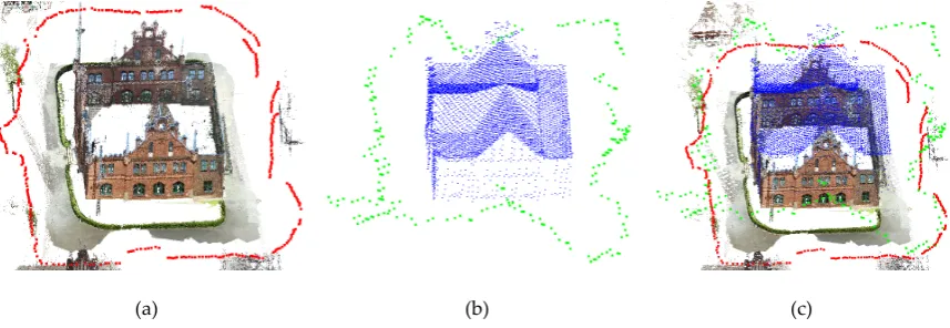
a horizontal transformation and a vertical transformation, as shown in Figure 4. 215
Figure 4. Overview of the accurate alignment process.
2D Façade Points Extraction from The Facade point cloud. Although most of the points in the facade 216
point cloud generated from ground images are on the façade part, there are inevitably many noise 217
points (such as trees, lamp-posts and passers-by), which will adversely affect the alignment. So, it is 218
essential to extract the real facade points from the facade point cloud, to reduce the adverse effect of 219
the noise points. Firstly, we extract candidate façade points of facade point cloud 𝓜 by using the 220
normal information. Since facade point cloud 𝓜 has been set to the upright direction in section 221
2.1.1, the dot product of normal 𝑁 of façade point 𝑝 and the upright vector (Z axis) should be 222
close to zero in an ideal case. Considering the error in the step of setting facade point cloud to upright, 223
we modify the condition to 𝑁 𝒁 < 0.01. Then, we refine the candidate façade points by using 224
their neighbour information. For each point 𝑝 (𝑥 , 𝑦 , 𝑧 ) in 𝓜 , it is considered as a façade point 225
⎩ ⎪ ⎨ ⎪ ⎧
(𝑥 − 𝑥 ) + (𝑦 − 𝑦 ) < 0.1 (max {𝑧 } − min {𝑧 })
2 < max {𝑧̂ } − min {𝑧̂ } count{𝑛 } > 10
(9)
The above equation means that real façade points should contain enough number of 227
neighbourhood points while these neighbourhood points’ height should distribute within a certain 228
range on the vertical direction. After the two steps, façade points 𝓜 are extracted from facade 229
point cloud 𝓜 and most noise point such as ground, grass, trees, lamp-posts and passers-by are 230
removed. Then, we project all points of 𝓜 into the plane of 𝑍 = 0 to obtain 2D façade points 231
𝓜 , as shown in Figure 5.(d). 232
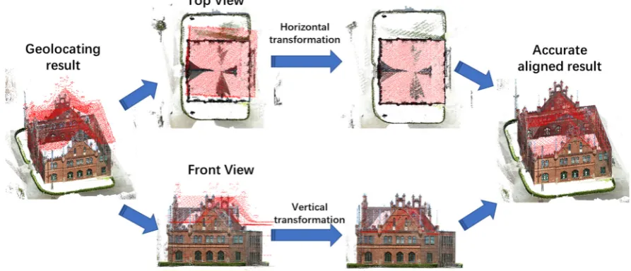
2D Boundary Points Extraction of Open Lidar Data. Alpha shape algorithm [34] is used to find the 233
boundary points from 2D LiDAR point cloud 𝓟 which is obtained by projecting LiDAR data into 234
to the horizontal plane. Firstly, alpha shapes with all possible alpha radius {𝑅 |𝑖 ∈ (1, 𝑁)} for 𝓟 235
are calculated. Then, once we find the critical alpha radius 𝑅 which can create a single region for 236
alpha shape, all alpha values above 𝑅 can be extracted as candidate alpha values {𝑅 }. Secondly, 237
we use a parameter 𝑊 to select one alpha value 𝑅 from {𝑅 }. Finally, the holes are filled after 238
creating the final alpha shape with alpha value 𝑅 . The points in the final alpha shape are considered 239
as the boundary point set 𝓟 , as shown in Figure 5.(b). 240
(a) (b) (c) (d)
Figure 5. Results of 2D façade points extraction and 2D boundary points extraction. Figure (a) and (c) 241
show the open LiDAR data and facade point cloud respectively. Figure (b) shows the boundary points 242
(top view) extracted from open LiDAR data and (d) shows the façade points (top view) extracted from 243
the facade point cloud. 244
Horizontal Alignment Using NC-CPD. From previous steps, 2D boundary points 𝓟 and 2D 245
façade points 𝓜 are extracted from open LiDAR data and facade point cloud, respectively. NC-246
CPD algorithm described in detail in section 2.2.2 is used to matching 𝓜 to 𝓟 . Firstly, we 247
calculate initial 𝜎 with 𝑹 = 𝑰, 𝑠 = 1, 𝒕 = 𝟎 . Initial 𝑆 in Equation (7) is also calculated with 𝑵𝒫 248
and initial 𝑵ℳ . Then, 𝑃 (𝑚|𝒙 ) in Equation (5) is calculated using 𝑹, 𝑠, 𝒕, 𝜎 , 𝑆 . Substitute 249
𝑃 (𝑚|𝒙 ) into Equation (6), 𝑹 , 𝑠, 𝑻, 𝜎 can be updated by minimizing Q in Equation (6). New 𝑆 250
can also be calculated by using new 𝑵𝒫 = 𝑵𝒫 ∙ 𝑹 . Repeat the previous steps until Q does not 251
change too much or a certain number of iterations is reached. After applying final transformation 252
X and Y axis direction are obtained. The registration process of NC-CPD is described in detail in 254
Figure 6. 255
Algorithm: Horizontal Alignment Using NC-CPD
Input: 2D boundary points 𝓟 and corresponding normal vector 𝑵𝒫 2D façade points 𝓜 and corresponding initial normal vector 𝑵ℳ Output: Accurate geolocated 2D façade points 𝓜
Initialization: Assign coarse alignment results: 𝑹 = 𝑰, 𝑠 = 1, 𝒕 = 𝟎, Calculate initial 𝜎 : 𝜎 = ∑ ∑ ||𝓟 − 𝓜 || ,
Construct initial normal consistency 𝑆 in Equation. (7)
EM optimization. repeat until convergence to obtain the final 𝑹𝒇, 𝑠 , 𝒕𝒇, 𝜎
E-step: Update 𝑝(𝑚|𝒙𝑛) with 𝑹 , 𝑠, 𝑻, 𝜎 , 𝑆
M-step: solve for the new 𝑹 , 𝑠, 𝑻, 𝜎 by minimizing Equation. (6)
The aligned 2D façade points is 𝓜 =𝑠 𝓜 𝑹𝒇𝑻+ 𝒕𝑻
Figure 6. The algorithm of horizontal alignment using CPD with normal consistency. 256
Then, after updating Z coordinates of façade points by applying 𝑠 𝑎𝑛𝑑 𝑡 , 3D façade point cloud 257
𝓜 is obtained. 258
Vertical Alignment. Façade point cloud has been accurately aligned to open LiDAR data on X and Y 259
axis direction by the horizontal alignment described in the previous section. A translation 𝑇 on the 260
vertical direction between 𝓜 and 𝓟 remain to be calculated. We calculate optimal 𝑇 by 261
matching corresponding boundary points respectively from 𝓟 and 𝓜 on the Z axis direction, 262
as following steps: (1). For one point 𝑝̅ (𝑥 , 𝑦 ) in 2D boundary points 𝓟 , we find 2D neighbour 263
point set {𝑝 , . . . , 𝑝 } and {𝑞 , . . . , 𝑞 } of 𝑝̅ with radius 0.1 meter, respectively from 𝓟 and 264
𝓜 . (2). Find the point 𝑝 and 𝑞 with maximum value on Z axis, respectively from {𝑝 , . . . , 𝑝 } 265
and {𝑞 , . . . , 𝑞 }, then calculate height difference 𝑇 = 𝑧 − 𝑧 . (3). For other point in 𝓟 , repeat 266
step (1) (2) to obtain height difference set {𝑇 , . . . , 𝑇 }. Then, the optimal 𝑇 is calculated by fitting 267
height difference set {𝑇 , . . . , 𝑇 }. Finally, applying translation 𝑇 to z coordinate of 𝓜 , accurately 268
aligned facade point cloud 𝓜 is obtained in the end. 269
3. Experiments and Discussion 270
3.1. Datasets Description 271
So far, there are currently no available benchmark datasets for fusing airborne LiDAR data and 272
facade point cloud generated from images. The proposed method is evaluated on a combined dataset: 273
1. Open LiDAR data of Dortmund in German which contain three experimental buildings 274
(Rathaus, Lohnhalle, Verwaltung) are downloaded from a Germany open data download portal [7]. 275
These open LiDAR data have been geolocated in the ETRS89 reference system with a UTM projection 276
with a point density of 25 points/m2.
277
2. Ground images of the three buildings come from a part of a benchmark dataset named “ISPRS 278
benchmark on multi-platform photogrammetry” [35] which can be downloaded from the official 279
website of ISPRS. These images are captured around the buildings using high-resolution digital 280
cameras on the ground. Due to the use of GPS locating accessories, image shooting positions are 281
recorded in these JPEG format images as GPS meta-data. Global coordinates of targets centers 282
distributed on the façade of the three buildings are provided for accuracy estimation. The details of 283
Table 1. Details of ground image datasets 285
Rathaus Lohnhalle Verwaltung
Images number 1211 194 351
Façade model points 36,085,050 8,004,604 11,176,836
Capturing device SONY NEX-7 Canon EOS 600D Canon EOS 600D
Focal length 16 mm 20mm 20mm
Image size (pixel) 4000 × 6000 5184 × 3456 5184 × 3456
Ground resolution 7.6 mm/pixel 3.1 mm/pixel 1.72 mm/pixel
GPS information
With GCP
3.2. Qualitative Analysis 286
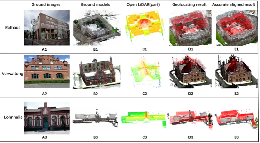
As shown in Figure 7, facade point clouds of Rathaus, Lohnhalle, Verwaltung (Figure.7 B1, B2, 287
B3) are generated from ground images (Figure.7 A1, A2, A3, image sample) using SfM and MVS 288
algorithms in COLMAP [32]. The open LiDAR data of the three buildings are visualized by height 289
rendering map in Figure.7 C1, C2, C3. It can be seen that there are no overlaps between open LiDAR 290
data and facade point clouds on their façade part except for Verwaltung, which has a small number 291
of points on the façades. But from another perspective, open LiDAR data and facade point clouds are 292
complementary, the former lack structural details on the façades, while the latter lack roof 293
information. 294
295
Figure 7. Datasets for evaluating the proposed method. From top to bottom, the different rows 296
respectively show the ground images (A), facade point clouds (B), open LiDAR (C), coarse alignment 297
result (D) and accurate alignment result (E) of Rathaus, Verwaltung and Lohnhalle. 298
The initial geolocation results which are not entirely accurate due to the low accuracy of GPS are 299
shown in Figure.7 D1, D2, D3, D4 (the red colour is assigned to open LiDAR data for better 300
recognition). After performing the accurate alignment step, the facade point clouds and open LiDAR 301
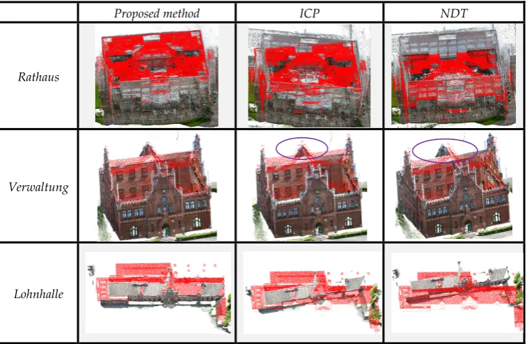
ICP and NDT algorithm, two classical algorithms of point set registration. The visualising results are 303
shown in Figure 8. Because of a relatively good density of points on the façades, we can see that ICP 304
and NDT achieve a relatively well result in Verwaltung comparing with Rathaus, Lohnhalle. 305
Surface reconstruction (Figure.9) was performed using the method in [36] to demonstrate the 306
effectiveness of our alignment algorithm. Both completeness and structural details are achieved in 307
the surface reconstruction after accurately aligning the facade point cloud to open LiDAR data. 308
Proposed method ICP NDT
Rathaus
Verwaltung
Lohnhalle
Figure 8. Fusion results of the proposed method comparing with ICP and NDT methods. 309
310
Figure 9. Poisson Surface reconstruction results. (a) Poisson Surface reconstruction from open LiDAR 311
data. (b). Poisson Surface reconstruction from façade point cloud generated from ground images. (c). 312
Poisson Surface reconstruction from fusion point cloud of open LiDAR data and façade point cloud. 313
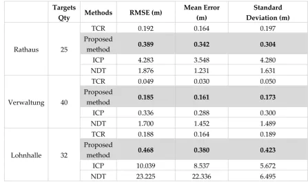
3.2. Quantitative Analysis 314
As shown in section 2.2, an iteration process is performed in the EM process to find the optimal 315
alignment result. After about less than 30 times iteration, the ratio of 𝑄 to initial 𝑄 quickly decline 316
to 1%, as shown in Figure 10. (a). Provided in the dataset of ‘ISPRS benchmark on multi-platform 317
photogrammetry’, accurate geographical coordinates {𝐺𝐶𝑃 } of target centers distributed on the 318
façade are used for quantitative evaluations of the alignment results, as shown in Figure 10.(b). We 319
estimate RMSE (root mean square error), mean errors and standard deviation between provided 320
global coordinates of target centers and their coordinates in the aligned results from different 321
methods, as shown in Table 2. 322
Figure 10. (a) Change of 𝑄 after each iteration. (b) Illustration of ground targets. 324
In fact, the error in the final geolocated facade point cloud includes errors from both the facade 325
point cloud generating process and the registration process. It is difficult to estimate the accuracy of 326
the registration process alone. In order to find the optimal geolocated results of façade point cloud 327
which include almost no registration errors, target centres registration (TCR) is performed by 328
estimating the rigid transformation 𝓣(𝑹, 𝑠, 𝑻) between the local coordinates of manually picked out 329
target centres and their provided global coordinates {𝐺𝐶𝑃 } using the least-square method. Due to 330
greatly reducing the registration errors by direct use of high-precision GCPs, errors in geolocating 331
the façade point cloud using TCR method can be referenced as errors from the facade point cloud 332
generating process. 333
Table 2. RMSE, ME and SD of the proposed method compared with other methods. 334
By analysing the errors of the different methods in Table 2, we can see that the proposed method 335
significantly improves the accuracy of test datasets comparing with ICP and NDT. It is well known 336
that Iterative Closest Point (ICP) [25] and Normal-Distributions Transform (NDT) [37] are effective 337
methods of point sets registration with large overlaps. Experiments have shown that ICP and NDT 338
methods cannot handle our datasets in which almost no overlaps can be found. So, errors up to 10 339
meters are obtained except for dataset of Verwaltung, which have a small number of points on the 340
(a) (b)
Targets
Qty Methods RMSE (m)
Mean Error (m)
Standard Deviation (m)
Rathaus 25
TCR 0.192 0.164 0.197
Proposed
method 0.389 0.342 0.304
ICP 4.283 3.548 4.280
NDT 1.876 1.231 1.631
Verwaltung 40
TCR 0.049 0.030 0.050
Proposed
method 0.185 0.161 0.173
ICP 0.336 0.288 0.300
NDT 1.700 1.452 1.489
Lohnhalle 32
TCR 0.188 0.164 0.189
Proposed
method 0.468 0.380 0.423
ICP 10.039 8.537 5.672
façade parts. Although not as good as the result of TCR methods, the proposed method achieves the 341
best accuracy compared to ICP and NDT methods due to the use of similarity on 2D outlines of 342
buildings. The accuracy of the proposed method is highly correlated with quality of façade point 343
cloud generated from images. For Rathaus, the farthest mean capture distance leads to an apparent 344
worst quality of façade point cloud from captured images (most significant errors in TCR method). 345
Consequently, a relatively large error appeared in dataset Rathaus using the proposed method. For 346
Lohnhalle dataset, we believe the disclosure of images captured around the target building cause the 347
relatively apparent errors in SfM process, even though the mean capture distance is much closer than 348
that of Rathaus dataset. However, the quality of the façade point cloud generated from images is 349
uncontrollable during the registration process, and how to improve it is beyond the scope of this 350
article. 351
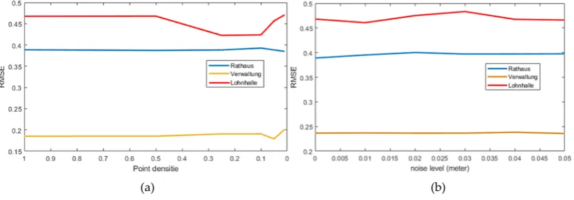
3.3. Robustness Analysis 352
It is known that different point densities and degrees of noise in the point clouds have a 353
significant impact on the performance of registration. We take several experiments on point clouds 354
mixed with different degrees of noise as well as point densities to test the robustness of the proposed 355
method. Fig. 12a–b illustrates the registration results achieved by the proposed method under 356
different degrees of noise and point densities. 357
Robustness to Point Densities. To evaluate the robustness of the proposed method to point density, 358
we randomly down-sample facade point cloud of Rathaus, Verwaltung and Lohnhalle from their 359
original point density to various densities. Different RMSEs evaluated between target centre 360
coordinates at different point density are given in Figure. 12 a. It can be seen that the proposed 361
method performed well even at 1% of the original point density, indicating the robustness of the 362
proposed method to different point densities. We attribute the robustness of our approach to different 363
point densities to the use of 2D similarity of building outlines in the registration between two sources 364
of point clouds. 365
Robustness to Noise. To evaluate the robustness of the proposed method to noise, Gaussian noise 366
with different standard deviations (1, 2, 3, 4, and 5 cm) was added to the point cloud data. The 367
different RMSE evaluated between target center coordinates under different levels of noise are shown 368
in Figure. 12b. Even when Gaussian noise with a standard deviation of 5 cm is added to the point 369
cloud, the proposed method achieved fine and stable accuracy. It indicates that the proposed method 370
is very robust to different levels of noise. We attribute the robustness of our approach to different 371
degrees of noise to the use of the probabilistic method in the accurate alignment. 372
(a) (b)
Figure 11. Robustness analysis of the proposed method. 373
4. Conclusion and Future Work 374
This paper presents an accurate and efficient framework for improving building façade details 375
framework is the alignment between limited overlapped facade point cloud generated from ground 377
images and open LiDAR point cloud. Experiments have shown that classic registration methods such 378
as ICP and NDT cannot handle our datasets in which limited overlaps can be found. Comparing with 379
ICP and NDT, the proposed method reduces the registration errors from up to 10 meters to less than 380
half a meter. We believe that our approach achieves good accuracy for the following reasons:(1). 381
Using Two-step strategies. Scale, translation and rotation differences are greatly relieved after coarse 382
alignment using GPS information of images. (2). Decompose registration into a horizontal 383
transformation and a vertical transformation instead of 3D registration directly. 2D overlapping 384
points on the contour of buildings are more stable for registration of the façade point cloud and 385
airborne point cloud than 3D overlapping points which can hardly be found between the two 386
different sources of point clouds. (3). The NC-CPD inherits the noise robust property of original CPD 387
algorithm. At the same time, it can handle the registration with structural ambiguities of buildings 388
by introducing normal consistency into the original CPD algorithm. 389
Both completeness and structural details of buildings in the open LiDAR data are significantly 390
improved after accurate alignment so that a complete and full resolution city building modelling and 391
other applications can be achieved. Our method can be extended to acquire images of different 392
buildings via crowdsourcing for improving façades details for open LiDAR data at city-scale. In the 393
future, we intend to carry larger trials with more terrestrial images of buildings via crowdsourcing. 394
Despite working well on many datasets, our method relies heavily on high-quality façade point cloud 395
generated from the SfM and MVS process in order to use the 2D outline information, which is the 396
only similarity between the two building point clouds. As such, the completeness and correctness of 397
façade point cloud require continuous improvement in image matching. 398
399 400
Acknowledgements: This work was partially supported by the National Natural Science Foundation of China 401
(No. 41271431, No. 41801390). 402
Author Contributions: The work presented here was carried out in collaboration among all authors. All authors 403
have contributed to this manuscript. Shenman Zhang is the primary author, having conducted the survey and 404
written the content. Pengjie Tao contributes to the analyse and discussion of an experiment as well as writing 405
and editing of the manuscript. 406
Conflicts of Interest: The authors declare no conflict of interest. 407
References 408
1. NYC Open Data. Available online: https://opendata.cityofnewyork.us/. 409
2. Open Data DC. Available online: http://opendata.dc.gov/. 410
3. Open Data of Canada. Available online: https://open.canada.ca/en/open-data. 411
4. Directive, I. N. S. P. I. R. E. Directive 2007/2/EC of the European Parliament and of the Council of 14 412
March 2007 establishing an Infrastructure for Spatial Information in the European Community 413
(INSPIRE). Publ. Off. J. 25th April 2007. 414
5. European Data Portal. Available online: https://data.europa.eu. 415
6. Scottish Remote Sensing Portal. Available online: https://remotesensingdata.gov.scot/. 416
7. Open NRW. Available online: https://open.nrw/open-data/. 417
8. Langheinrich, M. Evaluation of Gmsh Meshing Algorithms in Preparation of High-Resolution Wind 418
Speed Simulations in Urban Areas. Int. Arch. Photogramm. Remote Sens. Spat. Inf. Sci. 2018, 42. 419
9. Kersting, N. Open Data, Open Government und Online Partizipation in der Smart City. Vom 420
Informationsobjekt über den deliberativen Turn zur Algorithmokratie? In Staat, Internet und digitale 421
10. Degbelo, A.; Trilles, S.; Kray, C.; Bhattacharya, D.; Schiestel, N.; Wissing, J.; Granell, C. Designing 423
semantic application programming interfaces for open government data. JeDEM - eJournal eDemocracy 424
Open Gov. 2016, 8, 21–58. 425
11. Luebke, D.; Reddy, M.; Cohen, J. D.; Varshney, A.; Watson, B.; Huebner, R. Level of Detail for 3D 426
Graphics : Application and Theory. 2002, 431. 427
12. Furukawa, Y.; Ponce, J. [PVMS] Accurate, Dense , and Robust Multiview Stereopsis. 2010, 32, 1362– 428
1376. 429
13. Agarwal, S.; Snavely, N.; Simon, I.; Seitz, S. M.; Szeliski, R. Building Rome in a day. Proc. IEEE Int. 430
Conf. Comput. Vis. 2009, 72–79, doi:10.1109/ICCV.2009.5459148. 431
14. Shan, Q.; Curless, B.; Furukawa, Y.; Hernandez, C.; Seitz, S. M. Occluding contours for multi-view 432
stereo. In Proceedings of the IEEE Computer Society Conference on Computer Vision and Pattern Recognition; 433
2014; pp. 4002–4009. 434
15. Goesele, M.; Snavely, N.; Curless, B.; Hoppe, H.; Seitz, S. M. Multi-view stereo for community photo 435
collections xxx. Proc. ICCV 2007, 1–8, doi:10.1109/ICCV.2007.4408933. 436
16. Snavely, N.; Simon, I.; Goesele, M.; Szeliski, R.; Seitz, S. M. Scene reconstruction and visualization from 437
community photo collections. Proc. IEEE 2010, 98, 1370–1390, doi:10.1109/JPROC.2010.2049330. 438
17. Boulaassal, H.; Landes, T.; Grussenmeyer, P. Reconstruction of 3D Vector Models of Buildings By 439
Combination of Als, Tls and Vls Data. ISPRS - Int. Arch. Photogramm. Remote Sens. Spat. Inf. Sci. 2012, 440
XXXVIII-5/, 239–244, doi:10.5194/isprsarchives-XXXVIII-5-W16-239-2011. 441
18. Shan, Q.; Wu, C.; Curless, B.; Furukawa, Y.; Hernandez, C.; Seitz, S. M. Accurate geo-registration by 442
ground-to-aerial image matching. Proc. - 2014 Int. Conf. 3D Vision, 3DV 2014 2015, 525–532, 443
doi:10.1109/3DV.2014.69. 444
19. Wang, C.-P.; Wilson, K.; Snavely, N. Accurate georegistration of point clouds using geographic data. 445
3DTV-Conference, 2013 Int. Conf. 2013, 33–40, doi:10.1109/3DV.2013.13. 446
20. Agarwal, S.; Furukawa, Y.; Snavely, N. Building rome in a day. Commun. … 2011, 105–112, 447
doi:10.1145/2001269. 448
21. Rueckert, D.; Sonoda, L. I.; Hayes, C.; Hill, D. L.; Leach, M. O.; Hawkes, D. J. Nonrigid registration 449
using free-form deformations: application to breast MR images. 712 Ieee Trans. Med. Imaging 1999, 18, 450
712–21. 451
22. El-Hakim, S. F.; Beraldin, J. A.; Picard, M.; Godin, G. Detailed 3D reconstruction of large-scale heritage 452
sites with integrated techniques. IEEE Comput. Graph. Appl. 2004, 24, 21–29, 453
doi:10.1109/MCG.2004.1318815. 454
23. Yan, G.; Wen, D.; Olariu, S.; Weigle, M. C. Security challenges in vehicular cloud computing. In IEEE 455
Transactions on Intelligent Transportation Systems; 2013; Vol. 14, pp. 284–294. 456
24. Goshtasby, A. A. 2-D and 3-D image registration: for medical, remote sensing, and industrial applications; 457
John Wiley & Sons, 2005; ISBN 0471724262. 458
25. Besl, P. J.; McKay, N. D. A Method for Registration of 3-D Shapes. IEEE Trans. Pattern Anal. Mach. 459
Intell. 1992, 14, 239–256. 460
26. Brun, A.; Westin, C. Robust Generalized Total Least Squares; Springer Berlin Heidelberg, 2004; ISBN 978-461
3-540-22976-6. 462
27. Chetverikov, D.; Stepanov, D.; Krsek, P. Robust Euclidean alignment of 3D point sets: the trimmed 463
28. Stewart, C. V.; Chia-Ling Tsai; Roysam, B. The dual-bootstrap iterative closest point algorithm with 465
application to retinal image registration. IEEE Trans. Med. Imaging 2003, 22, 1379–1394, 466
doi:10.1109/TMI.2003.819276. 467
29. Kaneko, S.; Kondo, T.; Miyamoto, A. Robust matching of 3D contours using iterative closest point 468
algorithm improved by M-estimation. Pr 2003, 36, 2041–2047. 469
30. Campbell, D.; Petersson, L. An adaptive data representation for robust point-set registration and 470
merging. Proc. IEEE Int. Conf. Comput. Vis. 2015, 2015 Inter, 4292–4300, doi:10.1109/ICCV.2015.488. 471
31. Myronenko, A.; Song, X. Point set registration: Coherent point drifts. IEEE Trans. Pattern Anal. Mach. 472
Intell. 2010, 32, 2262–2275, doi:10.1109/TPAMI.2010.46. 473
32. Schonberger, J. L.; Frahm, J.-M. Structure-from-Motion Revisited. 2016 IEEE Conf. Comput. Vis. Pattern 474
Recognit. 2016, 4104–4113, doi:10.1109/CVPR.2016.445. 475
33. GPS Accuracy Available online: https://www.gps.gov/systems/gps/performance/accuracy/. 476
34. Edelsbrunner, H.; Mücke, E. P. Three-dimensional alpha shapes. ACM Trans. Graph. 1994, 13, 43–72, 477
doi:10.1145/174462.156635. 478
35. Nex, F.; Remondino, F.; Gerke, M.; Przybilla, H.-J.; Bäumker, M.; Zurhorst, A. ISPRS BENCHMARK 479
FOR MULTI-PLATFORM PHOTOGRAMMETRY. ISPRS Ann. Photogramm. Remote Sens. Spat. Inf. Sci. 480
2015, 2. 481
36. Kazhdan, M.; Hoppe, H. Screened poisson surface reconstruction. ACM Trans. Graph. 2013, 32, 1–13, 482
doi:10.1145/2487228.2487237. 483
37. Magnusson, M. The Three-Dimensional Normal-Distributions Transform --- an Efficient 484
Representation for Registration, Surface Analysis, and Loop Detection. Renew. Energy 2009, 28, 655– 485