Study Election Mode of Domicied Workers in Makassar City
Region
Rais Rachman1, Herman Parung2, Slamet Trisutomo3 and Nur Ali4
1
Doctoral Course Student, Civil Engineering Departement, Hasanuddin University, email : [email protected]
2
Professor, Civil Engineering Departement, Hasanuddin University, email : [email protected]
3
Professor, Architectural Engineering Departement, Hasanuddin University, email : [email protected]
4
Associated Professor, Civil Engineering Departement, Hasanuddin University, email : [email protected]
Abstract
The purpose of this study modeled the selection of the type of transport mode needed to travel to the outskirts of Makassar using Multinomial Logit Model In this study, the respondents entered into the model of multinomial logit is the overall respondent while the variables calculated in the equation is the type of transportation selected as a dependent variable and also some individual characteristics and travel characteristics as independent variables.
Results of processing with STATA version 12 program in which public transport means Pete-Pete serves as the base outcome, then produce a coefficient model of the mode selection utility for motorcycle taxi, private car and private motor. The obtained coefficients are then built into a model of the mode selection utility for the means of transportation of motorbikes, private cars and private motorcycles
Logarithmic regression result relation between distance and travel cost is found equation Y = 256 Ln (x) - 0,474 from this equation, it is known that the value of a relation between distance and travel cost is directly proportional where the bigger the travel distance is made, the bigger the trip cost will be Issued. However, based on the value of R2 = 0.49. This value is small, so it can be said that only 49% of the existing variants represent the actual conditions. While the Relationship Between Distance and Travel Time resulting from Logarithmic Regression is why = 5.548ln (x) - 5,002, from this equation it is known that the value of the relationship between distance and travel time is directly proportional where the greater the travel distance is done the more time The journey to be felt. The value of R2 = 0.510 can be said that 51% of existing variants represents the existing conditions significantly.
Keywords: Travel, Selection of modes, Means of transportation
1. Introduction
Growth in sub urban areas is faster than urban area growth. Various activities such as industrial centers and residential
centers are located in the suburbs. This is one of the factors that lead to rapid growth. The rapid development and diversion of land functions into settlements led to a high rate of movement, especially for working in the city center. This causes every workday a high rise of movement to reach the work location. In traveling to the workplace the workers are faced with a choice of types of modes of transportation, namely public transport such as Pete-Pete, motorcycle taxi and bumps and private transportation Transportation is said to be good if the travel time is fast enough and does not have accidents, the frequency of service is adequate, as well as safe (free from possible accident) and comfortable service conditions.
The choice of mode of transportation according to some transportation planning experts is considered the most important stage in transportation planning. The selection phase of this mode of transportation is the development of the model state of origin-destination, because when the stage of travel distribution determines the number of trips each zone of origin and destination, then at this stage of choice this mode to determine the number of trips that use various forms of conveyance (modes of transport) selection of this mode of transportation is one of the stages of the transportation planning process that is in charge of determining travel expenses or knowing the number (in terms of proportion) of persons and goods that will use or select the various modes of transportation available to serve a particular point of origin, For some specific travel purposes. The purpose of this study is to model the type of transportation mode needed to travel to the outskirts of Makassar using the Multinomial Logit Model.
2. Review of Literature
transport plan aims to find solutions to transportation problems in the most appropriate manner and use existing resources (Black, 1981). So transportation planning can be translated as a process undertaken to achieve the desired goal relationship with the development of transportation systems by utilizing resources effectively and efficiently. In the context of commuter transport planning, the purpose of transportation planning is how to accommodate commuter trips directed to the use of public transport, as well as to overcome the problems that have arisen due to commuting phenomena that prefer to use private vehicles. The process of transportation is a movement from the place of origin from which the transportation activity begins, to the destination, where transport activities are terminated (Nasution, 1996).
The development of the transportation system is a dynamic process and responding to changes in land use and socioeconomic behavior of the population. In the process of transportation needs planning known the existence of a close relationship between land use with the needs of transportation . In line with the development of a city community means the increasing number of people and the demands of society as a life support. The increasing number of urban residents and their activities has resulted in an increasing need for urban space. But the availability of space within the city remains fixed and limited, so that the increasing need for space for residence will always take up space in the suburbs (Yunus, 2005). The statement is clarified again by Chapin (1995) which states that the impact of an increase in population in a city, The development of the city will gradually expand to its peripheral regions.
Components in the transport system are divided into three systems, namely activity systems, network systems, and movement systems (Tamin, 2000). Taming (2000) explains that every land use or activity system (the first macro system) has certain types of activities that will generate movement and will attract movement in the process of fulfilling the needs. The system is a pattern system of land use activities consisting of patterns of social, economic, cultural, etc. Activities that arise in this system require transportation as a means of movement. Movement system is an interaction between activity system and network system that produces movement of human and or goods in the form of movement of a vehicle / person (Tamin, 2000). In order to smooth the movement or the process of moving people or goods from one place to another, then the three systems must be well organized. The three transportation systems are inseparable from the institutional influence that coordinates the three systems.
b. Factors Affecting Transportation Demand
Factors affecting the demand for transportation are an aspect of the consideration of the community in choosing the mode of transportation in the movement.
a) Characteristics of Travel Actors:
Characteristics of the traveler are characteristic of the user of the mode of transportation.
According to (J.DeD.Ortuzar and L.G. Willumsen in Amelia.2008) are as follows:
- Income Level
The income level will greatly influence a person in making the mode selection. The intended income level can be the income level of the head of the family or the total income of the family. For Indonesia, general information about income will be difficult to obtain, so it needs another indicator or measure such as the level of expenditure - Vehicle Ownership
In the presence of private vehicles in a household will give a person tend to travel by private vehicle as far as the public transport service is not enough representative for private vehicle owners.
- Density of Residential Development
Low-density urban areas will usually be occupied by households with middle to upper income levels, then the average ownership of vehicles is high. So that in carrying out daily activities has a tendency to use private transportation. Similarly vice versa with areas that have high density
- Other Socioeconomic Factors
In addition to the above factors, there are several other socioeconomic factors that are quite influential in the selection of modes, such as type of work, age, gender and others
- Ownership of driver's license - Household structure
c. Transport System Characteristics
Factors that are the benchmarks of transportation system characteristics include:
a) Travel Time, for public transport travel time consists of in vehicle time, waiting time, a time change of mode and access time. To make comparisons are usually used time relative is the comparison between travel time by public transport and travel time using private transportation.
b) Travel expenses, travel expenses of public transport are indicated by the applicable tariff rates. While the cost of travel by private transport will include many components, among others: the cost of fuel, lubricants, parking, tolls and others. As a measure of comparison, we use relative cost measures
d) Accessibility Index. Accessibility index is used to measure the quality of services provided by alternative modes, this index measures the ease of achieving an activity in a region.
d. Characteristics of Movement
Characteristics of movement or travel include the characteristics of the movement of the trip, which is influenced by:
a) The purpose of movement. The purpose of this movement becomes important such as, if the movement is made to the City then someone will choose public transportation because of better service level or use of motorcycles due to timeliness factor
b) Time of movement. By using private vehicles, especially motorcycles, the time required is flexible because it will be younger in traveling
c) Distance movement The farther the journey, a person tends to choose public transport compared to private transport.
e. Multinomial Logit Model
The multinomial logit (MNL) model is an extension of the dichotomous logit model. In the dichotomous logit model, the dependent variable consists of two categories (binary or dichotomy) While in the multinomial logit model, the dependent variable consists of 3 categories or more (polynomial). In this multinomial logit model we need some assumptions. First, the error in the utility component distributes Gumbel. Second, the error between alternative, alternatives is free. Third, errors between individuals are mutually free The multinomial logit model is commonly used to model choices, where the choice is not sorted and consists of 3 or more categories. McFadden (1974), Jonas A and Jan U (2010) proved that the multinomial logit model can be derived from the concept of utility, where individual decision-makers are observed 1 time (T = 1).
3. Research Design
The study discusses the model for selecting modes of the labor movement in the suburbs of the Makassar City based on positivism thinking. Research uses existing theory as a basis in the formulation of research variables used to search data in the field. The approach used is a quantitative approach, i.e. research that develops a study of a phenomenon by using mathematical models, theories and hypotheses related to a phenomenon. The use of quantitative data is more widely used in this research, so the method of analysis used in this research is quantitative and quantitative descriptive method.
Technique of collecting data which done consist of primary and secondary data collection. Primary data collection is through observation or direct observation using the five senses. Observations were made to obtain information about the clearer picture associated with the problem under investigation. Questionnaires distributed purposefully to commuters.
The questionnaire contains closed questions whose content direct the sample to the research objectives. Secondary data collection conducted such as literature review is the collection of information and data by reading and studying the literature related to research, as well as agency surveys such as surveys at the Central Bureau of Statistics (BPS).
a. Variables In Model
In this study, the respondents included in the multinomial logit model were all 1080 respondents. The variables calculated in the equation are the type of transportation chosen as the dependent variable and also some individual characteristics and travel characteristics as independent variables.
b. Utility Model Multinomial Logit
In the Multinomial Logit Model, the selection of public transport means Pete-Pete serves as the base outcome, so it will produce several models of equations. However, before generating the utility value of each model produced, it is first determined whether the resulting model has met the existing requirements, is seen from the significance value as well as other factors. Here is the model significance value of the STATA result
Multinomial logistic regression Number of obs = 1080 LR chi2 (66) = 156.55
Prob> chi2 = 0.0000
Log likelihood = -1164.6612 Pseudo R2 = 0.0630
From the value of LR chi2 (66)> 0 and the value of Prob> chi2 <0.005 it can be said that the model produced in this study has fulfilled the requirement, which means that the model generated from this STATA can already represent the real existing situation in the field.
4. Results and Discussion
a. Analysis of Results of Multinomial Logit Model The result of regression of STATA program utility model for the selection of public transport means ojek obtained value P> z value 0.005 is variable X5 (Work) and variable X15 (response of transportation performance to timeliness).
consider that the ojek performance against the timeliness is fast, the possibility of respondents to choose the motorcycle taxi as a means of transportation to travel on the job. The greater it is. While the regression model of STATA program utility model for the selection of private car transport means that the value of P> z value 0.005 is the variable X4 (work), X7 (travel cost) and X21 (performance of transportation means to the timeliness). This indicates that this variable has a significant effect on the selection of private car transportation. For the X7 variable that is travel cost, it is positive, so that it can be said that although the cost of travel is getting bigger but the opportunity to choose using private car means even greater This concerns the public's response to the performance of this means of transportation to the perceived timeliness. The result of regression of STATA program utility model for the selection of private transportation vehicle of motorcycles has value P> z 0,005 is variable X22 so it can be said that variable X22 that is responder responses about transportation performance to tariff / fuel cost have significant influence to the selection of bicycle transportation Motor for a work trip. With the value of the positive value coefficient means that the lower the cost tariff of motorbike beam it will be the greater the possibility of respondents choose motorcycles from travel work.
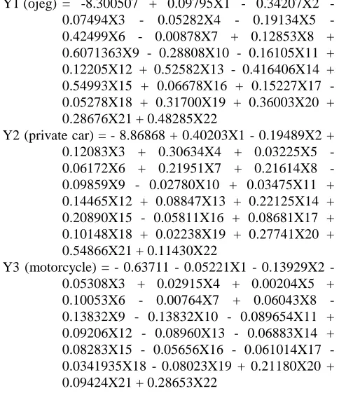
Of the three variables above, then the model generated for the needs of means of transportation is
Y1 (ojeg) = -8.300507 + 0.09795X1 - 0.34207X2 - 0.07494X3 - 0.05282X4 - 0.19134X5 - 0.42499X6 - 0.00878X7 + 0.12853X8 + 0.6071363X9 - 0.28808X10 - 0.16105X11 + 0.12205X12 + 0.52582X13 - 0.416406X14 + 0.54993X15 + 0.06678X16 + 0.15227X17 - 0.05278X18 + 0.31700X19 + 0.36003X20 + 0.28676X21 + 0.48285X22
Y2 (private car) = - 8.86868 + 0.40203X1 - 0.19489X2 + 0.12083X3 + 0.30634X4 + 0.03225X5 - 0.06172X6 + 0.21951X7 + 0.21614X8 - 0.09859X9 - 0.02780X10 + 0.03475X11 + 0.14465X12 + 0.08847X13 + 0.22125X14 + 0.20890X15 - 0.05811X16 + 0.08681X17 + 0.10148X18 + 0.02238X19 + 0.27741X20 + 0.54866X21 + 0.11430X22
Y3 (motorcycle) = - 0.63711 - 0.05221X1 - 0.13929X2 - 0.05308X3 + 0.02915X4 + 0.00204X5 + 0.10053X6 - 0.00764X7 + 0.06043X8 - 0.13832X9 - 0.13832X10 - 0.089654X11 + 0.09206X12 - 0.08960X13 - 0.06883X14 + 0.08283X15 - 0.05656X16 - 0.061014X17 - 0.0341935X18 - 0.08023X19 + 0.21180X20 + 0.09424X21 + 0.28653X22
b. Model Interpretation
For model interpretation, the positive sign (+) on the independent variable coefficient of the built model shows that the value of the independent variable is directly proportional to the dependent variable, for example, if the coefficient value x1 is positive (+), the higher the value of x1, and the highest also the value of the dependent variable, and vice versa, if the coefficient independent variable is marked negative (-), minus the value of the independent variable is inversely proportional to the dependent variable for example, if the coefficient value x1 is negative, meaning the higher the value of x1, the lower the value The dependent variable.
c. Average Transportation Values
After processing the data with the STATA program, obtained the average value of transportation means for each type of transportation means in review. Then by entering the average value of each of the previously calculated free variables into the equation of the utility model of the choice of transportation means that has been constructed, then the mode selection value can be obtained.
d. Utility Value
The utility value is the value generated from the equation formed. In this study, the value of variables is taken from the average value of each variable. The following table is the utility value of each equation.
Table 1. Utility value of transportation means
No Variable Value exp Value 1 y1 -1.04403789 0.352030348 2 y2 0.826329181 2.284915814 3 y3 1.348349993 3.851066
e. The probability value of each selection of means of transportation
The probability value of the means of transportation obtained through the use of the multinomial logit model obtained by processing the questionnaire based data stated preferences taken on each household in several urban villages in detail.
Relationship Between Variable Distance Against Variable Cost and Time of Time Relationship between Distance and Travel Costs as well as Distance and Time Travel is an interaction of travel characteristics that are considered very influential in terms of the selection of transportation facilities for the work of residents in the suburbs of Makassar.
f. The Relationship Between Distance and Travel Cost
The result of correlation analysis of distance and travel cost got correlation value between two variables worth 0,232. Based on this value, the correlation shown is not strong. Here are the results of linear regression and logarithmic regression.
1) Result of Linear Regression
From the results of linear regression analysis, then the equation produced is Y = 0,501x + 0,635.
2) Logarithmic Regression Result
From the result of logarithmic regression, we get the equation Y = 2,256 ln (x) - 0,474.
g. Relationship Between Distance and Travel Time
a) Result of Linear Regression
From the results of linear regression analysis, then the equation produced is Y = 0,501x + 0,635.
b) Logarithmic Regression Result
From the result of logarithmic regression, the equation Y = 2,256 ln (x) - 0,474.
h. Relationship Between Distance and Travel Time
a) Result of Linear Regeresi
Based on linear regression relation between distance with travel time, the equation become as follows Y = 1,176X - 2,002.
b) Logarithmic Regression Result
From result of Logarithmic regression analysis got equation Y = 5,548ln (x) - 5,002.
5. Conclusions
a. The Relationship Between Distance and Travel Cost a) The result of linear regression analysis shows the equation is Y = 0,501x + 0,635. This shows that the value of the relationship between distance and travel costs is directly proportional to where the greater the travel distance is done, the greater the travel costs to be incurred. However, based on the value of R2 = 0.54, including small, so it can be said that only 54% of existing variants represent the existing conditions significantly.
b) Based on the result of logarithmic regression, we get the equation Y = 2,256 ln (x) - 0,474. This suggests that the value of the relationship between distance and travel costs is directly proportional to where the greater the distance of travel work is done the greater the travel costs to be incurred. However, based on the value of R2 = 0.049. This value is small, so it can be said that only 4.9% of the existing variants represent the actual conditions.
b. Relationship Between Distance and Travel Time a) The result of linear regression relationship between the distance to travel time, the equation obtained as follows Y = 1.176X - 2.002, so it can be interpreted , that the value of the relationship between the distance and travel time is directly proportional, where the longer travel distance is done the longer the travel time That will be felt. The value of R2 = 0.508. This value is quite large so it can be said that 50.8% of the existing variants represent the existing conditions in real terms
b) While the results of the Logarithmic regression analysis found the equation Y = 5.548ln (x) - 5,002, so the value of the relationship between the distance and travel time is directly proportional where the greater the travel distance traveled, the greater the travel time will be felt. The value of R2 = 0.510 can be said that 51% of the variant That exists to represent the existing conditions in real terms.
References
1. Akbar, Arief. 2011. Review of the Selection of Motorcycle Modes and Public Transport of Mikrolet as Mode of Transportation for Working Journey (Case Study: KomuterBanyumanik-Semarang City Activity Center). essay. Department of Regional and City Planning, Faculty of Engineering, Diponegoro University. Semarang.
2. Amelia, Yanita. 2008. Travel between the 2 Cities by Comparing the Shuttle Service Modes, Trains, and Aircraft. Essay. Department of Civil Engineering. Faculty of Techni University of Indonesia. Depok. 3. Chapin, F. Stuart and Edward J. Kaiser. 1995. Urban
Landuse Planning. Fourth Edition. Chicago: University of Illinois Press
4. McFadden D., (1974). Conditional Logit Analysis of Qualitative Choice Behavior. Frontiers in Econometrics, Academic press, New York, pp.105-142.
5. Ramli, M.I., and Rachman, R., (2012) A departure time of the sub-urban work trips based on disutility minimizing approach. Proceeding of The 15 Fields of Transport Management and Management th FSTPT International Symposium, Bekasi, 23-24 November 2012.
6. Tamin O.Z., 2003, Transport Planning and Modeling, Bandung ITB Publisher.
First Author Rais Rachman is doctoral course student in Civil Engineering Departement of Hasanuddin University
Second Author Herman Parung is Professor in Civil Engineering Departement of Hasanuddin University
Third Author Slamet Trisutomo is Professor in Architectural Engineering Departement of Hasanuddin University.