Scholarship@Western
Scholarship@Western
Electronic Thesis and Dissertation Repository
7-14-2014 12:00 AM
A Spatial Analysis of Forest Fire Survival and a Marked Cluster
A Spatial Analysis of Forest Fire Survival and a Marked Cluster
Process for Simulating Fire Load
Process for Simulating Fire Load
Amy A. Morin
The University of Western Ontario
Supervisor
Dr. Douglas Woolford
The University of Western Ontario
Graduate Program in Statistics and Actuarial Sciences
A thesis submitted in partial fulfillment of the requirements for the degree in Master of Science © Amy A. Morin 2014
Follow this and additional works at: https://ir.lib.uwo.ca/etd
Part of the Applied Statistics Commons, and the Survival Analysis Commons
Recommended Citation Recommended Citation
Morin, Amy A., "A Spatial Analysis of Forest Fire Survival and a Marked Cluster Process for Simulating Fire Load" (2014). Electronic Thesis and Dissertation Repository. 2192.
https://ir.lib.uwo.ca/etd/2192
This Dissertation/Thesis is brought to you for free and open access by Scholarship@Western. It has been accepted for inclusion in Electronic Thesis and Dissertation Repository by an authorized administrator of
(Thesis format: Monograph)
by
Amy Morin
Graduate Program in Statistical and Actuarial Sciences
A thesis submitted in partial fulfillment
of the requirements for the degree of
Master of Science
The School of Graduate and Postdoctoral Studies
The University of Western Ontario
London, Ontario, Canada
c
The duration of a forest fire depends on many factors, such as weather, fuel type and fuel
mois-ture, as well as fire management strategies. Understanding how these impact the duration of
a fire can lead to more effective suppression efforts as this information can be incorporated
into decision support systems used by fire management agencies to help allocate suppression
resources. This thesis presents a thorough survival analysis of lightning and people-caused
fires in the Intensive fire management zone of Ontario, Canada from 1989 through 2004. The
analysis is then extended to investigate spatial patterns across this region using proportional
hazards Gaussian shared frailty models. The resulting posterior estimates suggest spatial
pat-terns across this zone. A fire load model is also developed by coupling a fire occurrence model
with a survival model and is explored via simulation. Marked cluster processes were found to
nicely capture the overall fire load trend over the fire season.
Keywords:Survival analysis, proportional hazards, frailty, marked cluster process, forest fires
Portions of this thesis are used in a paper which will be submitted to the International Journal
of Wildland Fire with Alisha Albert-Green, Dr. Douglas Woolford and Dr. David Martell,
who provided editing and comments on these sections. A second paper is also planned for
submission to Environmetrics; co-authors of this paper will include Dr. Douglas Woolford and
Dr. David Martell.
The financial support of the Natural Sciences and Engineering Research Council of Canada is
gratefully acknowledged. The Ontario Ministry of Natural Resources is also thanked for the
use of their fire weather data.
I am grateful to the faculty, staff and students in the Department of Statistical and Actuarial
Sciences at Western for a warm and welcoming learning environment. I would also like to
thank my committee members: Dr. Braun, Dr. Kulperger, Dr. Hong and Dr. Zitikis, for
dedi-cating time to my thesis examination and for providing helpful revisions.
Helpful conversations and revisions from our collaborators Alisha Albert-Green and Dr. David
Martell are also much appreciated. In addition, Dr. Charmaine Dean is thanked for welcoming
me to the lab, and for providing computing equipment and funding.
Dr. Douglas Woolford is particularly recognized for devoted supervision and patience
through-out this degree. He has gone through-out of his way to help me get to this point and his guidance
con-tinues to lead me to new opportunities.
I wish to sincerely thank my office mates: Alisha, Erin, Mark, and Phil, for always being
open to share insightful advice and knowledge. I will forever cherish my time at Western with
these friends.
I am eternally grateful to my family, especially my parents, Jean-Pierre and Gis`ele, for
lov-ingly and unselfishly supporting me throughout my life. Lastly, I owe my deepest gratitude to
John for always being there and believing in me.
Abstract ii
Co-Authorship Statement iii
Acknowledgements iv
List of Figures vii
List of Tables x
1 Introduction 1
2 The Data and Study Area 4
2.1 Forest Fire Data . . . 4
2.2 Fire Management and Weather Variables . . . 9
3 Methodology 11 3.1 Survival Analysis . . . 11
3.1.1 The Survival Time,T . . . 11
3.1.2 The Kaplan-Meier Estimator . . . 12
3.1.3 Log-Location-Scale Models . . . 12
3.1.4 The Cox Proportional Hazards Model . . . 14
3.1.5 The Proportional Hazards Shared Frailty Model . . . 15
3.1.6 Model Selection . . . 16
3.2 Point Processes . . . 17
3.2.2 Non-Homogeneous Poisson Processes . . . 17
3.2.3 Parent-Child Cluster Processes . . . 18
3.2.4 Estimatingλ(t) . . . 18
4 Results 20 4.1 Survival Analysis . . . 20
4.1.1 Kaplan-Meier Estimator . . . 20
4.1.2 Log-Location-Scale Models . . . 20
4.1.3 Cox Proportional Hazards Model . . . 24
4.1.4 Proportional Hazards Shared Frailty Model . . . 26
4.1.5 Goodness of Fit . . . 33
4.2 Fire Arrival Modelling . . . 38
4.2.1 Non-Homogeneous Poisson Process . . . 38
4.2.2 Parent-Child Cluster Processes . . . 39
4.2.3 Fire Load Simulation . . . 42
5 Conclusion 47 5.1 Discussion . . . 47
5.2 Future Work . . . 51
Bibliography 53
Curriculum Vitae 55
2.1 Ontario’s fire management zones prior to 2004. . . 5
2.2 The typical timeline of the area burned by a fire through its progression phases
with (blue) and without (black) suppression efforts. . . 6
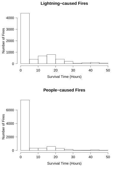
2.3 Histograms of the survival time, in hours, of lightning (top panel) and
people-caused fires (bottom panel) which are declared under control within 2 days. . . 8
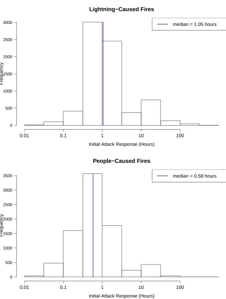
2.4 Histograms of the initial attack response time, in hours, of lightning (top panel)
and people-caused fires (bottom panel). . . 10
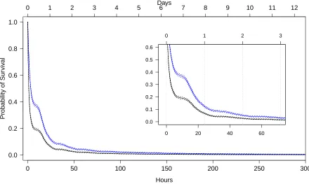
4.1 Kaplan-Meier survival curves of lightning (blue lines) and people-caused fires
(black lines) with 95% confidence limits (dashed lines). . . 21
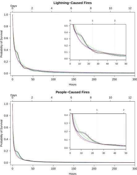
4.2 KM estimates (solid black lines) with 95% confidence limits (dashed black
lines) and Weibull (green lines), lognormal (blue lines) and loglogistic (red
lines) estimates of survival probabilities of lightning-caused fires (top panel)
and people-caused fires (bottom panel). . . 22
4.3 Fitted survival curves of lightning (top panel) and people-caused (bottom panel)
fires at covariate values representative of a typical fire, as fit by the AFT Weibull
model (blue lines) and the KM estimates (solid black lines) of survival
proba-bilities with 95% confidence limits (dashed black lines). . . 25
4.4 Fitted survival curves of lightning (top panel) and people-caused (bottom panel)
fires at covariate values representative of a typical fire, as fit by the Cox PH
model (blue lines) and the KM estimates (solid black lines) of survival
proba-bilities with 95% confidence limits (dashed black lines). . . 28
4.6 Choropleth maps of lightning-caused fires where each FMC is assigned a heat
map colour based on its frailty term. The top panel uses evenly spaced intervals
and the bottom panel uses an interval length equal to the standard deviation of
the random effects. . . 31
4.7 Choropleth maps of people-caused fires where each FMC is assigned a heat
map colour based on its frailty term. The top panel uses evenly spaced intervals
and the bottom panel uses an interval length equal to the standard deviation of
the random effects. . . 32
4.8 Profile likelihood-based 95% confidence intervals of the variance of the random
effects. . . 34
4.9 The parameter estimates of the compartment-specific fixed effects (top panel)
and the posterior estimates, in reference to FMC-15, from the frailty model
(bottom panel) of lightning-caused fires. . . 36
4.10 The parameter estimates of the compartment-specific fixed effects (top panel)
and the posterior estimates, in reference to FMC-15, from the frailty model
(bottom panel) of people-caused fires. . . 37
4.11 The 95th percentiles of daily fire arrivals over the fire season from 1000 runs
of a simulated non-homogeneous Poisson process (blue line) and from the true
data (black line). . . 39
4.12 The estimated time-dependent rate from a Poisson GAM with day of year effect
fit to the presence/absence of fires. . . 40
4.13 The 95th percentiles of daily fire arrivals over the fire season from 1000 runs
of a simulated Bartlett-Lewis process (blue line) and from the true data (black
line). . . 41
ated by the non-homogeneous Poisson (2nd row), Bartlett-Lewis (3rd row) and
Neyman-Scott (bottom row) processes. . . 43
4.15 The 95th percentiles of daily fire arrivals over the fire season from 1000 runs
of a simulated Neyman-Scott process (blue line) and from the true data (black
line). . . 44
4.16 Fire arrivals (segments) and survival times (length of segments) over the fire
season (top panel) and the associated daily fire load (bottom panel) from a
single run of the simulation. . . 46
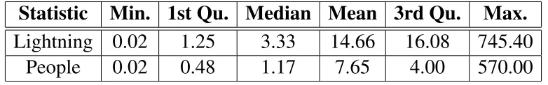
2.1 Descriptive statistics of the survival time (in hours) of fires from the Intensive
zone, by ignition cause. . . 7
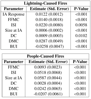
4.1 Parameter estimates, standard errors (Std. Errors) and p-values from the fitted
AFT Weibull models of lightning (top panel) and people-caused (bottom panel)
fires. . . 23
4.2 Parameter estimates, standard errors (Std. Errors) and p-values from the fitted
Cox PH models of lightning (top panel) and people-caused (bottom panel) fires. 24
4.3 The AIC and marginal decrease in AIC at each stage of the forward selection
of covariates in the Cox PH models of lightning (top panel) and people-caused
(bottom panel) fires. . . 27
4.4 Parameter estimates, standard errors (Std. Errors) and p-values of the fixed
ef-fects from the fitted proportional hazards shared frailty model of lightning (top
panel) and people-caused fires (bottom panel). . . 30
4.5 A comparison of the average number of fire days and fires per fire season, with
standard deviations in parentheses, from the historical data and the Poisson
process simulation. . . 38
4.6 A comparison of the average number of fire days and fires per fire season, with
standard deviations in parentheses, from the historical data, the Bartlett-Lewis
simulation, and the Neyman-Scott simulation. . . 42
Introduction
The duration of a forest or wildland fire influences the area burned in Canadian forests. To
reduce the area burned, forest fires which are difficult to extinguish are of particular interest
as they pose a significant threat to forest resources across much of the Province of Ontario,
Canada. A better understanding of the variables which contribute to longer lasting forest fires
could be incorporated into decision support systems used by fire management agencies to
pri-oritize fires and allocate suppression resources.
In Canada, forest fires are ignited by lightning or by people. The ignition risk of
lightning-caused fires depends heavily on the moisture within the top layer of the forest floor, which is
often referred to as the dufflayer, where a fire can smoulder until the surface of the forest floor
becomes dry enough to sustain its spread (Wotton and Martell, 2005). By contrast, the ignition
of people-caused fires is most dependent on the moisture of the fine litter fuels on the surface
of the forest floor (Wotton, 2009). Consequently, lightning and people-caused fires have been
modelled separately in the literature (Wotton and Martell, 2005; Wotton et al., 2003). The
ap-plications in this paper model lightning-caused fires and people-caused fires separately.
In this thesis, we use survival analysis methods to explore how fire weather variables affect
the duration of a forest fire. For the purpose of this study, we define thedurationof a forest
fire to be the time interval from the beginning of initial attack action to the time that the fire is
declared as being under control, which we will hereafter refer to as the survival time. Survival
analysis is often employed to investigate time to some significant event (Lawless, 2003), often
in the presence of censoring and/or truncation, commonly in biostatistics and engineering. In
the biostatistics literature, the event of interest is often death or the recurrence of a disease
(e.g., Fleming and Lin, 2000), while time to product failure is often the event of interest in
engineering applications (e.g., Tsai et al., 2003). In our application, the event of interest is the
time at which a fire is declared under control.
In addition to the traditional applications, survival analysis has been applied to the lifetimes
of living organisms, including animals (Johnson et al., 2004) and trees (Ritchie et al., 2007),
extensively in ecology. However, the application of survival analysis to wildland fires has been
focused on estimating fire frequency and fire cycles involving the time required to burn an area
equal in size to the studied area (Larsen, 1997; Senici et al., 2010) by modelling the time since
a fire occurred at specific points on the landscape. In this thesis, we investigate the associations
between fire weather variables and the distribution of the survival time of a forest fire by the
means of a thorough survival analysis. We also explore the data, looking for spatial patterns in
the duration of forest fires. The objective of this research is to provide forest fire managers with
an alternative fire weather modelling technique which could be incorporated in their strategic,
tactical and operational planning systems.
To forest fire managers, thefire load represents the magnitude of the suppression efforts and
resources corresponding to fires that occur in a specific area and over a specified time interval
(Martell, 2007). In this thesis, we will specify the fire load on a given day of the fire season
to be the number of fires burning on the landscape. A simulation of the fire load is performed
by coupling a fire occurrence model with one of our survival models for a single region. The
fire occurrence is modelled using a non-homogeneous Poisson process and special forms of
the stochastic cluster processes as a mark. These types of models have been used extensively
to model ecological occurrences including rainfall (Rodriguez-Iturbe et al., 1987) and
earth-quakes (Ogata, 1988).
The remainder of this thesis is organized as follows. A description of the study area, data and
Ontario’s fire management system is given in Chapter 2. Exploratory data analyses are also
performed. In Chapter 3, we present definitions, statistical concepts and methods which will
be applied in the study. Simple parametric log-location-scale models are then fit to the data in
Chapter 4, along with survival models that incorporate the effects of other covariates. In
addi-tion, spatial patterns across our study region are analyzed using proportional hazards Gaussian
shared frailty models and illustrated using choropleth maps. We also present the development
of a stochastic fire load model via simulation. We conclude the study with a discussion of our
The Data and Study Area
The Aviation, Forest Fire and Emergency Services (AFFES) Branch of the Ontario Ministry
of Natural Resources (OMNR) is responsible for forest fire management on Crown land in
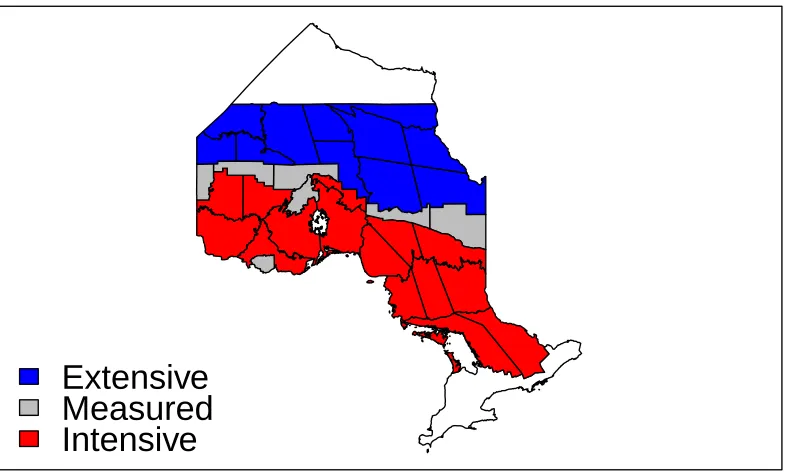
the fire region of the Province of Ontario. Prior to 2004, this fire region (coloured area) was
partitioned into the three fire management zones shown in Figure 2.1, each of which received
different levels of protection. The strategy in the Intensive zone was to suppress all fires as soon
as suppression resources were available, in the Measured zone fires were initially attacked and
re-evaluated if extended attack was needed for containment, and in the Extensive zone fires
were left to burn so long as they did not threaten a community. Recently, the number of
zones and their corresponding management strategies have been modified (see OMNR, 2004).
Consequently, we focus our analysis on historical records of fires prior to this change in the
provincial fire management strategy.
2.1
Forest Fire Data
We studied the lifetimes of 18,183 forest fires in the Intensive zone of the Province of Ontario,
for the period 1989 through 2004, using data provided by the OMNR. That fire archive
in-cludes many fire attributes including the dates and times at which each fire was reported, when
suppression action began and when the fire was declared under control. It also includes other
Extensive
Measured
Intensive
Figure 2.1: Ontario’s fire management zones prior to 2004.
information such as the weather, vegetation or fuel type and fuel moisture associated with each
fire. Among the fires we studied, 43% were caused by lightning and 57% were caused by
peo-ple.
Martell (2007) described how fire management agencies track a forest fire’s progress through
several distinct phases. The life cycle of a fire begins with ignition, sometime later it is
de-tected and later reported to the fire management agency. Once the fire has been reported, the
duty officer or dispatcher prioritizes it, places it in the initial attack (IA) queue and dispatches
initial attack resources (e.g., airtankers and fire fighters) to begin initial attack action. A fire is
declared to be in a state of being held when it is no longer spreading but may possibly resume
spreading, and subsequently deemed under control when adequate control lines have been
es-tablished around the fire’s perimeter. The fire crews then work on extinguishing the fire from
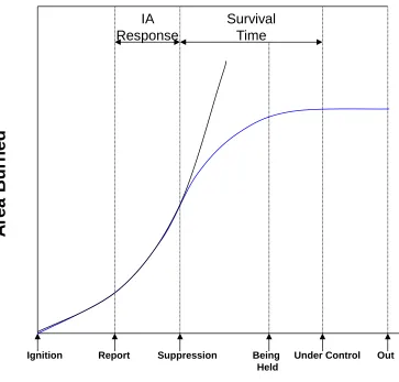
at which point the fire is then declared as out. Figure 2.2 displays the importance of effective
suppression efforts in terms of area burned over a typical fire’s lifetime (Parks, 1964). From
this figure, it is clear that understanding survival time is important, because area burned is
pro-portional to this quantity.
Ignition Report Suppression Under Control Out
A
re
a
Burned
IA Response
Survival Time
Being Held
Figure 2.2: The typical timeline of the area burned by a fire through its progression phases with (blue) and without (black) suppression efforts.
As mentioned previously in this thesis, we define a fire’s survival time as the time between
when initial attack begins and when the fire is declared under control. These times are used
estimated) and the amount of time that it takes to bring the fire under control is of most interest
and use to fire management agencies. This survival time is measured in hours, where decimal
places represent minutes, for our analysis. Fires with negative survival times (870 fires) that
resulted from data coding errors are removed, as well as those where the initial attack and
under control dates and times are the same (133 fires). Apart from simple data entry error,
negative survival times might have occurred because the time at which a fire was declared as
under control was not specified along with the date. In this situation, the time is recorded as
midnight which leads to problems when working with time differences between date-stamps
of short fires. Fires which have survival times of length 0 may be caused by similar mistakes
or by a fire crew arriving at a fire and deciding that suppression is not needed due to the low
intensity of the fire and expected weather (rain). These fires are removed from the dataset as in
this study we are only interested in fires which need to be suppressed.
The OMNR considers an initial attack to have been successful if a fire is brought to a state
of being held by noon on the day following the day the fire was reported or if final size is less
than 4 hectares. Roughly 97.5% of fires in Ontario are successfully contained by the initial
attack force. For this reason, the 3 fires with survival times which are greater than 1,000 hours
(just under 42 days) are removed. Some summary statistics for the data we analyze are
dis-played in Table 2.1 and histograms of the survival time of lightning and people-caused fires
which are declared under control within 2 days are displayed in Figure 2.3.
Statistic
Min. 1st Qu. Median Mean 3rd Qu.
Max.
Lightning
0.02
1.25
3.33
14.66
16.08
745.40
People
0.02
0.48
1.17
7.65
4.00
570.00
Lightning−caused Fires
Survival Time (Hours)
0 10 20 30 40 50
0 1000 2000 3000 4000
Number of Fires
People−caused Fires
Survival Time (Hours)
0 10 20 30 40 50
0 2000 4000 6000
Number of Fires
2.2
Fire Management and Weather Variables
Theinitial attack responseis the time between when a fire is reported and the time that initial
attack action begins. Figure 2.4 displays the histograms of the response time (in hours) for
lightning and people-caused fires. Investigation of the effect of this covariate on the survival
time of forest fires is motivated by the potential impact it may have on the final size of fires.
The size (in hectares) of a fire at the start of initial attack is also considered.
Canadian forest fire managers use the Canadian Forest Fire Danger rating System (CFFDRS)
to assess the impact of weather on fire occurrence and behaviour processes. We will be using
5 of the codes and indices from the CFFDRS that represent the cumulative impact of weather
on the moisture content of different components of a forest fuel complex and potential fire
behaviour. A thorough overview of the CFFDRS for the purpose of modelling is provided by
Wotton (2009). The Fine Fuel Moisture Code (FFMC) is a numerical rating of the moisture in
the small, readily consumed, fine fuels on the forest floor. It increases with increasing dryness
varying from saturation to a completely dry surface layer. The Initial Spread Index (ISI) is a
rating of the potential rate of spread of a fire and is based upon the wind speed and the FFMC.
The larger the ISI, the greater the fire spread rate potential. The DuffMoisture Code (DMC)
is a measure of the moisture content of the top 7 cm of the forest floor where litter starts to
decay and ranges from 0 (full saturation) from where it can increase with no upper bound. The
Drought Code (DC) is a measure of moisture content of deep layers of the forest floor and of
dead woody debris approximately 18 cm thick and accounts for long-term drying. The higher
the DC, the drier the deep organic fuel. The Build-Up Index (BUI) is a weighted mean of DMC
and DC and serves as a measure of the potential fuel available for consumption on and in the
forest floor. It is also a useful indicator of difficulty in extinguishing smouldering fires. These
fire weather variables have been historically used in forest fire occurrence prediction models;
notable examples include the logistic regression models of Woolford et al. (2011) and Wotton
Lightning−Caused Fires
Initial Attack Response (Hours)
Frequency
0 500 1000 1500 2000 2500 3000
0.01 0.1 1 10 100
median = 1.05 hours
People−Caused Fires
Initial Attack Response (Hours)
Frequency
0 500 1000 1500 2000 2500 3000 3500
0.01 0.1 1 10 100
median = 0.58 hours
Methodology
3.1
Survival Analysis
3.1.1
The Survival Time,
T
The survival time,T, is a continuous and non-negative random variable which represents the
time to an event. In the analysis of lifetimes, one is most interested in the probability of
survival,S(t)= P(T > t), and the hazard rate,λ(t)= Sf((tt)), where f(t) is the probability density
function of T. In the context of our research, we analyze the probability distribution for the
time until a fire is declared under control, given that it is being suppressed. Here, the hazard
or failure rate can be viewed as the probability that a fire would “die” at time t, conditional
on its survival to that point. In this sense, it can be viewed as the instantaneous rate that the
fire becomes under control. The hazard rate is important because the survival function can be
expressed as a function of this rate as
S(t)=exp
− t Z 0 λ(u)du .
The remainder of Section 3.1 reviews common non-parametric, parametric and semi-parametric
methods to estimate survival probabilities or hazard rates. The proportional hazards shared
frailty model and inference procedures are also introduced.
3.1.2
The Kaplan-Meier Estimator
The Kaplan-Meier (KM) estimator approximates the underlying continuous lifetime
distribu-tion using a discrete distribudistribu-tion (Lawless, 2003). It is a non-parametric (i.e., no assumpdistribu-tions
about the underlying distribution are made) technique. Estimates are made at each of the
ob-served event times. The KM estimator of the survival function is defined as
ˆ
SK M(t)= Y j:tj≤t
1− dj Yj
!
, t≥0,
wheretj denotes the observed event times, dj is the number of events which occurred at time
tj and Yj is the number of subjects at risk at time tj, j = 1, ...,n. Note that dj/Yj is a
non-parametric estimator of the hazard function sincedj/nestimates f(tj) andYj/nestimatesS(tj).
3.1.3
Log-Location-Scale Models
Log-location-scale models are a class of parametric models commonly used to model lifetime
data. The lifetime random variable, T, has a log-location-scale model if its survival function
can be written in the form
S(t)=S0
log(t)−u b
! ,
whereS0is a fully specified survival function with positive support andu∈Randb> 0 are the
location and scale parameters which shift and affect the spread of the distribution, respectively.
The three most commonly used log-location-scale models are the Weibull, lognormal, and
loglogistic. They are obtained when S0(t) is the extreme value, normal, or logistic survival
function, respectively. The location and scale parameters are estimated from the data using
parameters for a given parametric model. For complete data, the likelihood function of n
observations x1, ...,xnis
L≡ L(θ)= n
Y
i=1
f(xi;θ),
where f is the density function of the parametric model with parameter vector θ. The
max-imum likelihood estimates of the parameters are obtained by maximizing the log-likelihood
function,l(θ)=logL(θ).
Non-parametric survival estimates can be used as a method of comparing models (Lawless,
2003). Using this approach, the appropriateness of each log-location-scale parametric model
can be determined by examining how closely the fitted survival probabilities follow the KM
estimates. Non-parametric models are useful comparison tools as they are true to the data and
only make the assumption that the data are independent; they do not impose a distribution upon
the data.
The KM estimator and log-location-scale methods produce simpler models in the sense that
they don’t incorporate effects of other independent variables or covariates. The accelerated
failure time(AFT) model is a parametric regression model which takes into account the effect
of covariates on the survival function. It is a log-location-scale distribution of the form
S(t|x)= S0
logt−u(x) b
! ,
where the location parameter is dependent on the covariate vector,x, and is often assumed to
be a linear function of pcovariates. That is,u(x)= p
P
i=1
βixi, where theβ’s are parameters to be
estimated. The AFT model makes the assumption that the effect of covariates is equivalent to
altering the rate at which time passes. If the linear function of the covariates, u(x), is greater
survival probability across time. Similarly, ifu(x)< 0 then the covariate vector is accelerating
the time scale or decreasing the survival probability across time.
3.1.4
The Cox Proportional Hazards Model
The Cox proportional hazards (PH) model is a widely used semi-parametric method for survival
analysis that can incorporate covariate effects. The hazard rate is modelled as
λj(t|xj)=λ0(t)ex
0
jβ, j= 1, ...,n
where jindexes the observations,λ0is the baseline hazard rate, xj is the covariate vector and
β is the associated parameter vector of length p. The baseline hazard rate can be viewed as
the hazard function when all covariates are 0. The covariates then have a multiplicative effect
on this baseline. In this application of the Cox PH model, our main interest is in quantifying
the effects of the covariates. The Cox PH model is commonly built using forward selection
of covariates, details of which will be provided in Section 3.1.6. The effect of the covariates,
ex0jβ, is parametrically estimated without considering the baseline by maximizing Cox (1972,
1975)’s partial likelihood,
L(β)= n
Y
j=1
ex0jβ
P
kRj
ex0kβ
,
where Rj is the set of observations which are at risk for an event (fires not under control) at
the time of the jth observation. This likelihood is partial as it involves only the parameters of
interest and the baseline hazard is considered a nuisance function which subsequently may be
non-parametrically estimated using estimators given by Breslow (1972) or Efron (1977), for
example. If parameterized in terms of the survival function, the Cox PH model takes the form
Sj(t |xj)= S0(t)e
x0 jβ
3.1.5
The Proportional Hazards Shared Frailty Model
The purpose of frailty models is to describe the excess risk, or frailty, for distinct categories.
The main idea is that there are greater correlations among data within these categories or
clus-ters. In the application of the Cox Proportional Hazards model, these within cluster
dependen-cies cause non-proportionality of the hazards and loss of precision of the estimated
parame-ters. This problem is remedied by implementing a multivariable mixed-effects survival model,
namely the shared frailty model. The shared frailty model is such that each observation
be-longs to only one of the distinct categories, all observations within a category share a common
frailty, and the frailties from different categories are independent (Therneau et al., 2003). The
hazard rate from the proportional hazards shared frailty model is
λi j(t)= λ0(t)ex
0
i jβ+ωi, j=1, ...,n
i, i=1, ...,s
where jindexes the observations in categoryi, xi j is the covariate vector of length pwith
as-sociated parameter vectorβ and ωi is the random effect term of category i. The distribution
and mean of the random effects must be specified, while the variance is left unspecified. The
choice of the distribution of the random effects is based on the dependence structure present in
the data being modeled. In practice, the most common choices include the gamma distribution
with mean 1 and the normal distribution with mean 0, the latter of which will be applied in this
thesis as it allows flexibility in modelling data with various dependence structures. We will
also demonstrate that this normal frailty term is appropriate for our data later in this thesis. In
the case of shared frailty models, where each observation belongs to only one category and the
observations within a category have a common random effect term, s
P
i=1
ni =n.
Penalized regression models are used to estimate Cox PH models with frailty terms (Ripatti
and Palmgren, 2000). When fitting such models, the random effects are added to survival
distribution. The penalized partial log-likelihood, `ppl, consists of adding a penalty function,
`penalty, to the partial log-likelihood,`partial, as a constraint as follows:
`ppl = `partial−`penalty
= s
X
i=1
ni
X
j=1
log
ex0i jβ+ωi
P
qwRi j
ex0
qwβ+ωq
−`penalty.
In the case of normally distributed random effects with mean 0 and variance γ, the penalty
function is 12 s
P
i=1
ω2 i
γ +log(2πγ)
. The tuning parameter of the penalty function is the random
effect variance,γ, which penalizes for extremely large absolute values ofωi.
The parameter estimation is done by starting with an initial guess of ˆγ, and using the
Newton-Raphson method to solve forβˆ and ˆωi from the estimating equations based on the first partial
derivatives of the penalized partial log-likelihood above. Then,βandωiare fixed at these
max-imized values and an estimating equation based on the approximate marginal log-likelihood is
solved for a new value of ˆγ, more details of which may be found in Ripatti and Palmgren
(2000). These two steps are iterated until convergence.
3.1.6
Model Selection
Model selection aims to find the subset of covariates which will result in the best fitting model.
Forward selection is a model building approach which applies a stepwise search algorithm (see
e.g., Venables and Ripley, 2002) in order to select covariates through the use of the Akaike
information criterion (AIC), where a smaller AIC represents a better fit (Therneau and
Gramb-sch, 2000). Beginning with the null model, the covariate which decreases the AIC the most
is added to the model, one at a time, until the addition of any remaining covariates does not
decrease the AIC. In the case of close fits, this method establishes a preference for simpler
3.2
Point Processes
This section introduces point process methods and estimation procedures with emphasis on
simulation procedures.
3.2.1
Homogeneous Poisson Processes
A point process is a stochastic process of point occurrences. When the points are restricted
to vary only temporally, the process is called “on the line” which refers to the time-axis. The
homogeneous Poisson process is the simplest point process where the points occur completely
randomly in time. This process has independent non-overlapping time increments and the
number of events in any such increment of length a, N(a), has a Poisson distribution with
rateλa, whereλis the intensity of the Poisson process. The times between any 2 points, the
increment lengths, are independent and exponentially distributed with rateλ. The simulation
of a homogeneous Poisson process is therefore straightforward.
3.2.2
Non-Homogeneous Poisson Processes
A non-homogeneous Poisson process has an intensity which varies temporally,λ(t). For this
process, the number of events in the increment (a,b] has a Poisson distribution with rate b
R
a
λ(t)dt and non-overlapping increments are independent. In contrast to the homogeneous
Poisson process, the number of events in an increment is dependent on its start and end points,
along with its length; this makes the process non-stationary.
Thinning, introduced by Lewis and Shedler (1979), is a convenient method for simulating a
non-homogeneous Poisson process. It involves simulating a homogeneous Poisson process
with constant rate function,λu, which dominates the desired rate function,λ(t), for alltin the
desired interval. A generated point at time t is then independently rejected with probability
n
uniform random variable,ui, for each generated pointiand reject the point ifui >
λ(ti) λu .
3.2.3
Parent-Child Cluster Processes
Acluster processconsists of a point process which generates cluster origins (parents) and
an-other point process which associates points (offspring) to each parent with specified location
about the parent (Cox and Isham, 1980). The overall cluster process may or may not include
the parents as points in practice, but it is of note that these parents are purely conceptual and
do not have physical representations.
The Bartlett-Lewis process is a special cluster process in which a Poisson process generates
the parents, a point process generates the offspring of each parent, and the offspring are
po-sitioned such that the increments between points are independent and identically distributed
according to some distribution, starting from the parent. The Neyman-Scott process differs
from the Bartlett-Lewis only in that the offspring are independently and identically distributed
away from the parent. For both cluster processes, there is typically a stopping rule either for
the total number of points generated, or for the number of offspring generated for each cluster
parent.
3.2.4
Estimating
λ
(
t
)
The intensity of the non-homogeneous Poisson process will be estimated using a Poisson
gen-eralized additive model(GAM), first introduced by Hastie et al. (1986). This regression model
relates the conditional mean of the response,µ= µ(x), to a linear combination of smooth
func-tions of covariates,x, using the log link function. For a single covariate,x, this model takes the
form:
whereβ0is the intercept which is estimated parametrically and f is a smooth function, which,
in our application is estimated using a thin plate regression spline (Duchon, 1977) basis.
Penal-ized iteratively reweighted least squares, conditional on a smoothing parameter, is implemented
to fit the model, details of which may be found in Wood (2006). The smoothing parameter is
estimated by generalized cross-validation.
The results from the implementation of the methods introduced in this chapter will be
Results
4.1
Survival Analysis
The methods discussed in Section 3.1 are implemented in R using the survival package of
Therneau (2014) and the results are presented in the remainder of this section.
4.1.1
Kaplan-Meier Estimator
The KM estimates of the survival curves of both lighting-caused and people-caused fires are
displayed in Figure 4.1. Examination of these curves clearly shows that people-caused fires
tend to have smaller survival probabilities and reveals two noticeable periods at which the
curves exhibit a short-lived plateau rather than continually decreasing as expected. These
plateaux occur near the 8 and 32 hour marks which suggests that they may be caused by
sup-pression being stalled overnight.
4.1.2
Log-Location-Scale Models
The Weibull, the lognormal, and the loglogistic survival models are plotted for lightning-caused
fires and people-caused fires in Figure 4.2. These results suggest that the fits of these parametric
models are reasonable, however they do not adequately capture the features demonstrated by
0 50 100 150 200 250 300 0.0
0.2 0.4 0.6 0.8 1.0
Hours
Probability of Sur
viv
al
Days
0 1 2 3 4 5 6 7 8 9 10 11 12
0 20 40 60
0.0 0.1 0.2 0.3 0.4 0.5 0.6
n
n
0 1 2 3
0 50 100 150 200 250 300 0.0 0.2 0.4 0.6 0.8 1.0 Hours
Probability of Sur
viv
al
Lightning−Caused Fires Days
0 2 4 6 8 10 12
0 10 20 30 40 50 60
0.0 0.1 0.2 0.3 0.4 0.5 n n
0 1 2
0 50 100 150 200 250 300
0.0 0.2 0.4 0.6 0.8 1.0 Hours
Probability of Sur
viv
al
People−Caused Fires Days
0 2 4 6 8 10 12
0 10 20 30 40 50
0.0 0.1 0.2 0.3 0.4 n n
0 1 2
the KM estimates in the left-tails of the distributions. This suggests that models which account
for the effect of covariates should be explored. Examining the AIC values for each of these
fitted models suggests that the Weibull distribution is the preferred log-location-scale model
for both types of fires. Therefore, this distribution is employed to fit AFT models, the results
of which are summarized in Table 4.1.
Lightning-Caused Fires
Parameter
Estimate (Std. Error)
P-Value
IA Response
0.0122 (0.0012)
<
0.001
FFMC
0.0140 (0.0018)
<
0.001
ISI
0.0220 (0.0080)
0.0058
Size at IA
0.0006 (0.0002)
<
0.001
DC
0.0009 (0.0003)
0.0102
DMC
0.0287 (0.0049)
<
0.001
BUI
-0.0258 (0.0047)
<
0.001
People-Caused Fires
Parameter
Estimate (Std. Error)
P-Value
FFMC
0.0093 (0.0023)
<
0.001
ISI
0.0518 (0.0068)
<
0.001
Size at IA
0.0587 (0.0044)
<
0.001
DC
0.0028 (0.0004)
<
0.001
DMC
0.0242 (0.0065)
<
0.001
BUI
-0.0207 (0.0061)
<
0.001
Table 4.1: Parameter estimates, standard errors (Std. Errors) and p-values from the fitted AFT Weibull models of lightning (top panel) and people-caused (bottom panel) fires.
The implementation of forward selection (e.g., Venables and Ripley, 2002) results in fitting
the model for lightning-caused fires with all covariates included, while the model for
people-caused fires includes all variables except the initial attack response time. All parameter
esti-mates, with the exception of BUI, are positive which suggests that increases in these variables
with the KM estimates and 95% confidence limits of the survival curves, are displayed in
Fig-ure 4.3. These graphs suggest that the parametric AFT models over-smooth the data and do
not adequately capture the characteristics which were displayed by the KM estimates of the
survival curves. These log-location-scale models do, however, appear to do an adequate job of
describing the overall trend in survival probability.
4.1.3
Cox Proportional Hazards Model
The Cox PH model, as described in Section 3.1.4, is fit to the survival time of lightning and
people-caused fires. The same covariates as in the AFT models are selected. The summaries of
the fitted models for lightning-caused fires and people-caused fires are displayed in Table 4.2.
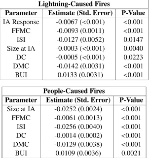
Lightning-Caused Fires
Parameter
Estimate (Std. Error)
P-Value
IA Response
-0.0067 (
<
0.001)
<
0.001
FFMC
-0.0093 (0.0011)
<
0.001
ISI
-0.0127 (0.0052)
0.0147
Size at IA
-0.0003 (
<
0.001)
0.0040
DC
-0.0005 (
<
0.001)
0.0223
DMC
-0.0142 (0.0031)
<
0.001
BUI
0.0133 (0.0031)
<
0.001
People-Caused Fires
Parameter
Estimate (Std. Error)
P-Value
Size at IA
-0.0252 (0.0024)
<
0.001
FFMC
-0.0061 (0.0013)
<
0.001
ISI
-0.0256 (0.0040)
<
0.001
DC
-0.0014 (0.0002)
<
0.001
DMC
-0.0129 (0.0038)
<
0.001
BUI
0.0109 (0.0036)
0.0021
0 20 40 60 80 0.0
0.2 0.4 0.6 0.8 1.0
Lightning−Caused Fires
Hours
Probability of Sur
viv
al
0 10 20 30 40
0.0 0.2 0.4 0.6 0.8 1.0
People−Caused Fires
Hours
Probability of Sur
viv
al
Similarly to the AFT model, all parameter estimates, except BUI, are negative which indicates
a decreased hazard rate, or equivalently, an increased survival time with increasing
parame-ter values. The positive BUI parameparame-ter estimate is likely due to a dependence between it and
another variable. Table 4.3 displays the marginal improvements in the AIC at each stage of
the forward selection of covariates in these Cox PH models. The structure of the implemented
stepwise selection guarantees an improvement in fit at each stage, however overfitting may
oc-cur. A general rule of thumb to avoid overfitting is that a marginal decrease in the AIC of less
than 2 suggests that there is not substantial evidence which indicates a gain of information in
the model with the additional covariate, relative to the previous model (Burnham and
Ander-son, 2004). Based on this rule, the Cox PH models of both lightning and people-caused fires
would not include DMC and BUI.
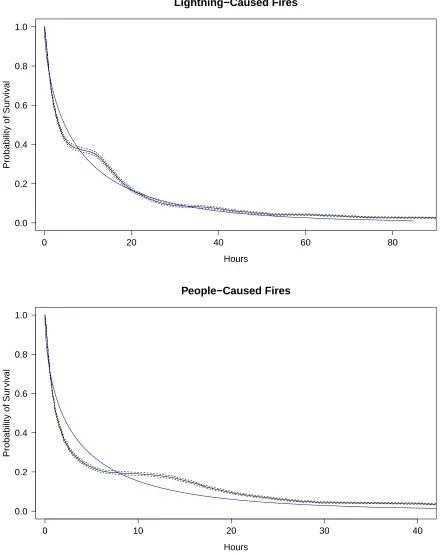
Figure 4.4 displays the fitted Cox PH survival curves of lightning and people-caused fires (with
all selected covariates), along with the KM estimates and 95% confidence limits of the survival
curves. These graphs suggest that the Cox PH models capture the important characteristics
which were displayed by the KM estimates of the survival curves. The Cox PH model is more
flexible than the AFT model because its baseline distribution is left unspecified.
4.1.4
Proportional Hazards Shared Frailty Model
The Cox proportional hazards model assumes that the effects of covariates on the baseline
haz-ard rate is proportional over time (with vertical shifts) and that the survival times of fires are
independent; these assumptions will be violated when there is correlation among certain fires.
Since the Province of Ontario has vast forest landscapes, the survival times of fires will be
af-fected differently by the previously modeled covariates in dissimilar regions, thereby creating
spatial correlation between fires within similar sections of Ontario. Martell and Sun (2008)
par-titioned the province into small polygons referred to asfire management compartments(FMCs)
Lightning-Caused Fires
Model
AIC
Marginal Decrease
Null
115304.7
-IA Response
115108.6
196.1
FFMC
114939.8
168.8
Size at IA
114924.2
15.6
ISI
114916.5
7.7
DC
114913.6
2.9
DMC
114913.1
0.5
BUI
114893.9
19.2
People-Caused Fires
Model
AIC
Marginal Decrease
Null
133389.9
-Size at IA
133137.7
252.2
ISI
132988.0
149.7
DC
132874.5
113.5
FFMC
132854.1
20.4
DMC
132852.8
1.3
BUI
132845.1
7.7
Table 4.3: The AIC and marginal decrease in AIC at each stage of the forward selection of covariates in the Cox PH models of lightning (top panel) and people-caused (bottom panel) fires.
management zones in Ontario, displayed in Figure 2.1, with a digital map of the forest sections
from the forest region classification system of Rowe (1972). Conditional on these
compart-ments, the survival times of the fires may now be appropriately modeled as each FMC can be
assumed to be approximately internally homogeneous with respect to ecological characteristics
such as fuel, weather and topography as well as fire management strategy. The implementation
of a shared frailty model, in which each fire belongs to only one compartment and the fires
within a compartment have a common random effect, allows the assumption that the fires have
0 20 40 60 80 0.0
0.2 0.4 0.6 0.8 1.0
Lightning−Caused Fires
Hours
Probability of Sur
viv
al
0 10 20 30 40
0.0 0.2 0.4 0.6 0.8 1.0
People−Caused Fires
Hours
Probability of Sur
viv
al
A semiparametric PH shared frailty model with zero-mean normally distributed random effects
is fit to lightning and people-caused fires by maximizing the penalized partial likelihoods as
described in Section 3.1.5. The fixed effects used in these models are the same as in the
non-frailty models to allow for appropriate comparisons. The parameter estimates, standard errors
and p-values of the fixed effects from the fitted models are displayed in Table 4.4.
Lightning-Caused Fires
Parameter
Estimate (Std. Error)
P-Value
IA Response
-0.0067 (0.0008)
<
0
.
001
FFMC
-0.0092 (0.0012)
<
0
.
001
ISI
-0.0103 (0.0052)
0.047
Size at IA
-0.0002 (0.0001)
0.009
DC
-0.0004 (0.0002)
0.067
DMC
-0.0150 (0.0031)
<
0
.
001
BUI
0.0127 (0.0031)
<
0
.
001
People-Caused Fires
Parameter
Estimate (Std. Error)
P-Value
FFMC
-0.0060 (0.0013)
<
0
.
001
ISI
-0.0253 (0.0040)
<
0
.
001
Size at IA
-0.0249 (0.0024)
<
0
.
001
DC
-0.0014 (0.0002)
<
0
.
001
DMC
-0.0128 (0.0038)
<
0
.
001
BUI
0.0104 (0.0036)
0.004
Table 4.4: Parameter estimates, standard errors (Std. Errors) and p-values of the fixed effects from the fitted proportional hazards shared frailty model of lightning (top panel) and people-caused fires (bottom panel).
The posterior estimates of the random effects, ˆωi, from each FMC are extracted from the model
and applied to create the choropleth maps in Figures 4.6 and 4.7. The exponentiated posterior
estimates are interpreted as multiplicative factors on the hazard rate. Negative posterior
Frailty by Fire Management Compartment
of Lightning−Caused Fires
( −0.35 , −0.25 ] ( −0.25 , −0.15 ] ( −0.15 , −0.05 ] ( −0.05 , 0.05 ] ( 0.05 , 0.15 ] ( 0.15 , 0.25 ] ( 0.25 , 0.35 ] ( 0.35 , 0.45 ]
Frailty by Fire Management Compartment
of Lightning−Caused Fires
(−0.345,−0.172] (−0.172,0.172] (0.172,0.345] (0.345,0.517]
Frailty by Fire Management Compartment
of People−Caused Fires
( −0.25 , −0.15 ] ( −0.15 , −0.05 ] ( −0.05 , 0.05 ] ( 0.05 , 0.15 ] ( 0.15 , 0.25 ]
Frailty by Fire Management Compartment
of People−Caused Fires
(−0.254,−0.127] (−0.127,0.127] (0.127,0.254]
probability. As such, the choropleth maps apply the brightest red color of the heat palette to
compartments with the largest negative posterior estimates to imply greater fire danger through
to the palest yellow being applied to compartments with the largest positive posterior estimates
to imply the least fire danger.
The choropleth maps of people-caused fires do not display clear or easily interpretable trends,
however the choropleth maps of lightning-caused fires have interesting patterns. The use of
evenly-spaced intervals in the top panels allow the visualization of specific patterns. There is
a slight west to east gradient which is noticeable in the Intensive zone of the evenly-spaced
lightning-caused fires map (Figure 4.6, top panel). The bottom panels allow the visualization
of more broad spatial patterns by using interval lengths which represent standard deviations of
the random effects. The map of lightning-caused fires with standard deviation-based intervals
(Figure 4.6, bottom panel) reinforces that in the Intensive zone, the western region experiences
fires with shorter survival times.
4.1.5
Goodness of Fit
The construction of a profile likelihood-based confidence interval is used as a preliminary
as-sessment of the frailty term’s significance. For a sequence of random effect variances, the
like-lihood ratio (LR) test statistics are computed and plotted at each fixed variance. A horizontal
line is added to the plot 3.84 units below the test statistic value of the fitted frailty model, which
corresponds to a chi-squared test on 1 degree of freedom. The intersections of the horizontal
line and the profile likelihood produce a profile likelihood-based 95% confidence interval for
the variance of the random effects. The resulting plots, displayed in Figure 4.8, suggest that
the frailty terms of the models are significant in terms of this preliminary assessment since
the confidence intervals are relatively narrow. It is of note that the confidence interval for the
variance of the random effects from the frailty model of lightning-caused fires is narrower than
0.00 0.02 0.04 0.06 0.08 0.10 600
650 700 750
Profile Likelihood of Lightning−Caused Fires
Variance of Random Effects
LR test
0.00 0.02 0.04 0.06 0.08 0.10
280 300 320 340 360 380 400
Profile Likelihood of People−Caused Fires
Variance of Random Effects
LR test
Therneau and Grambsch (2000) suggests that the significance of the frailty term is more
strongly evaluated by a likelihood ratio test comparing the integrated-likelihood of the frailty
model, where the frailty terms are integrated out of the likelihood, to the Cox PH fitted
likeli-hood without a frailty term. Based on this comparison, both the lightning and people-caused
frailty models are significant improvements on the respective proportional hazards models
without frailty term. However, it is of note that this chi-squared test is conservative since
the frailty terms,eω, are constrained to be greater than or equal to zero.
Next, the suitability of the normality assumption of the frailty model is verified by fitting the
Cox PH model with additional fixed effects for the FMCs. FMC-15, the compartment in the
western region which experiences the most lightning-caused fires, is chosen as the baseline
compartment. To make the choropleth maps from the frailty model comparable to those from
the fixed effects model in Figures 4.9 and 4.10, FMC-15’s posterior estimate is subtracted from
the other posterior estimates such that the values are representative of the multiplicative diff
er-ence on the hazard rate of fires in FMC-15. The fixed effect parameter estimates are similar to
the posterior random effect estimates which suggests that this modelling is robust to violation
Fixed Effect Parameter Estimates
of Lightning−Caused Fires
15
(−0.78,−0.62] (−0.62,−0.47] (−0.47,−0.31] (−0.31,−0.16]
Frailty Comparison to FMC15
of Lightning−Caused Fires
15
(−0.78,−0.62] (−0.62,−0.47] (−0.47,−0.31] (−0.31,−0.16]
Fixed Effect Parameter Estimates
of People−Caused Fires
15
(−0.56,−0.42] (−0.42,−0.28] (−0.28,−0.14] (−0.14,0.02]
Frailty Comparison to FMC15
of People−Caused Fires
15
(−0.56,−0.42] (−0.42,−0.28] (−0.28,−0.14] (−0.14,0.02]
4.2
Fire Arrival Modelling
The modelling in the remainder of this section will be implemented on lightning-caused fire
occurrences from 1963 through 2004. Our study region is restricted to FMC-15 such that the
modelling is purely temporal.
4.2.1
Non-Homogeneous Poisson Process
A Poisson GAM with a thin-plate spline for a day of year effect is fit to the daily number of
fires. The resulting time-dependent rate is used to generate fire arrivals (fires which have been
reported) according to a non-homogeneous Poisson process. This simulation is facilitated by
thinning realizations from a homogeneous Poisson process as described in Section 3.2.2. The
resulting 95th percentiles of daily fire arrivals over 1000 simulated fire seasons and the true data
are displayed in Figure 4.11. Inspection of this figure suggests that the intensity of the Poisson
process is too small, especially near the peak (middle) of the fire season, due to the large
num-ber of days with 0 fires in the data. Table 4.5 indicates that the average numnum-ber of fires per fire
season from the simulation is similar to that of the historical data, while the average number
offire days, defined as days with 1 or more fires, per fire season from the simulation is much
larger than the historical data. This discrepancy implies that the generated fires are too spread
out and that there are not enough fires generated on the same day. An intuitively appealing way
of modelling the inherent clustering of the arrival of lightning-caused fires is by the means of
a parent-child cluster process, which will be implemented in the next section.
Average No. Fire Days Average No. Fires
Historical
29.60 (15.97)
77.50 (78.76)
Poisson Process
58.09 (5.40)
78.23 (8.41)
100 150 200 250 300 0
2 4 6 8 10 12
Non−Homogeneous Poisson Process Simulation
Day of Year
Number of Fires
Simulation Data
Figure 4.11: The 95th percentiles of daily fire arrivals over the fire season from 1000 runs of a simulated non-homogeneous Poisson process (blue line) and from the true data (black line).
4.2.2
Parent-Child Cluster Processes
The implemented Bartlett-Lewis process is assumed to have the following two-component
structure. A non-homogeneous Poisson process of rate λ(t), which is dependent on the day
of year, generates the cluster origins (parent fires), and for each parent, offspring are generated
according to a homogeneous Poisson process of rateβwithin 1 day from the time of the parent
fire arrival. The generated parents are also assumed to be fires, which implies that if 0 offspring
are generated for a parent, the associated cluster consists of a single fire. This cluster process
couples the two individual components independently; implications of this assumption are
dis-cussed in Chapter 5.
The rate of the non-homogeneous Poisson process,λ(t), is estimated by fitting a Poisson GAM,
days). The resulting time-dependent rate is displayed in Figure 4.12. A simple Poisson model
is fit to the daily fire counts from the zero-truncated data. The resulting estimated rate, ˆβ,
rep-resents the offspring intensity, given a fire day has been observed. These estimated parameters
are used to simulate the Bartlett-Lewis process 1000 times and the 95th percentiles of daily fire
arrivals over the fire season from the simulation and true data are displayed in Figure 4.13.
100 150 200 250 300
0.0 0.1 0.2 0.3 0.4
Poisson GAM of Fire Days
Day of Year
λ
tFigure 4.12: The estimated time-dependent rate from a Poisson GAM with day of year effect fit to the presence/absence of fires.
The Bartlett-Lewis process specifies that the intervals between successive points are iid, which
was achieved by generating the offspring according to a homogeneous Poisson process. By
contrast, the Neyman-Scott process positions points such that they are iid from the cluster
ori-gin. This is achieved by generating offspring arrival times away from the parent fires using
independent truncated exponential( ˆβ) random variables (truncated above 1 day). In this case,
a stopping rule which involves a count of offspring is more suitable as this process does not
100 150 200 250 300 0
2 4 6 8 10 12
Bartlett−Lewis Process Simulation
Day of Year
Number of Fires
Simulation Data
as ˆβ. Since βis the expected number of offspring over 1 day from the homogeneous Poisson
process in the Bartlett-Lewis process, the total expected number of fires from the two cluster
processes are equivalent. Figure 4.14 displays 2 historical fire seasons (1983 and 1998), along
with 2 fire seasons generated by each of the non-homogeneous Poisson, Bartlett-Lewis and
Neyman-Scott processes. This Neyman-Scott process is simulated 1000 times and the 95th
percentiles of daily fire arrivals over the fire season from the simulation and true data are
dis-played in Figure 4.15.
Figures 4.13 and 4.15 illustrate that parent-child cluster models improve the simulated arrivals
during the peak of the fire season as compared to the simple arrival process. The clustering
also significantly improves the average number of fire days per season, displayed in Table 4.6,
as they are closer to the historical value than the single Poisson process simulation.
Average No. Fire Days Average No. Fires
Historical
29.60 (15.97)
77.5 (78.76)
Bartlett-Lewis
37.91 (6.27)
78.22 (15.94)
Neyman-Scott
37.17 (6.49)
78.45 (14.58)
Table 4.6: A comparison of the average number of fire days and fires per fire season, with standard deviations in parentheses, from the historical data, the Bartlett-Lewis simulation, and the Neyman-Scott simulation.
4.2.3
Fire Load Simulation
A simulation of the fire load, the number of fires burning on the landscape, over a fire season
is accomplished by generating observations from a marked cluster process, where the survival
times are independent marks associated with points from the cluster process. For each arrival
time generated from the Bartlett-Lewis process, a survival time is simulated from the Weibull
100 150 200 250 300 0 2 4 6 8 10 12
Historical Fire Season
Day of Year
Number of Fires
100 150 200 250 300
0 2 4 6 8 10 12
Historical Fire Season
Day of Year
Number of Fires
100 150 200 250 300
0 2 4 6 8 10 12
Poisson Process Simulation
Day of Year
Number of Fires
100 150 200 250 300
0 2 4 6 8 10 12
Poisson Process Simulation
Day of Year
Number of Fires
100 150 200 250 300
0 2 4 6 8 10 12 Bartlett−Lewis Simulation
Day of Year
Number of Fires
100 150 200 250 300
0 2 4 6 8 10 12 Bartlett−Lewis Simulation
Day of Year
Number of Fires
100 150 200 250 300
0 2 4 6 8 10 12 Neyman−Scott Simulation
Day of Year
Number of Fires
100 150 200 250 300
0 2 4 6 8 10 12 Neyman−Scott Simulation
Day of Year
Number of Fires
100 150 200 250 300
0
2
4
6
8
10
12
Neyman−Scott Process Simulation
Day of Year
Number of Fires
Simulation Data
typical fire. The top panel of Figure 4.16 displays each fire arrival and its survival time for a
single run of this simulation, along with the associated daily fire load over the fire season in the
bottom panel.
The results presented in this chapter will be discussed, followed by future work, in the next
100 150 200 250 300 0
20 40 60 80
Simulated Arrivals
Day of Year
Fire Number
100 150 200 250 300
0 2 4 6 8
Simulated Fire Load
Day of Year
Fire Load
Conclusion
5.1
Discussion
We have presented a thorough survival analysis in the context of exploring the associations
between fire weather covariates and the distribution of the survival time of a forest fire, along
with an investigation of spatial patterns. In doing so, we have illustrated that the survival times
of forest fires are dependent on fire weather variables. The initial attack response time between
a fire being reported and the start of initial fire suppression efforts, and the fire’s size at initial
attack were statistically significant when modelling hazard rates for forest fires in Ontario. The
simple (i.e., no covariates) parametric log-location-scale models failed to capture the
plateaux-like features observed in the left-tail of the survival distributions. Although incorporating the
effect of covariates using Weibull AFT models led to improvements in fit, the estimated survival
curves were quite smooth and again failed to capture the important characteristics displayed
in the KM curves. The results from the Cox PH model were found to closely resemble the
plateaux noticed in the KM curves and this was seen for both lightning and people-caused
fires. Operationally, the left-tail of the distribution is important as most fires are declared under
control within 1 or 2 days from the onset of initial attack.
In our analysis of historical forest fire data, all variables considered were included in the model
for lightning-caused fires; the fitted model for people-caused fires did not include the initial
attack response time. This supports the conjecture, and the basis of fire management, that the
longer the initial attack response time, the larger a fire becomes and the more difficult it is to
get under control. Figure 2.4 illustrated that the initial attack response time for people-caused
fires, as compared to lightning-caused fires, does not tend to be as long. This may be a result
of people-caused fires being smaller in size at the time of initial attack and because they tend
to occur near populated areas which makes them easier to access by suppression crews and
equipment. Lightning-caused fires also tend to arrive in clusters due to passing storm systems
(Woolford and Braun, 2007). This may result in multiple fires on the landscape, in relatively
close proximity to each other, which can overwhelm the fire management crews who have
lim-ited suppression resources, resulting in longer initial attack response times before suppression
action begins on some of those fires.
Each of the parameter estimates from the Cox PH models, with the exception of BUI, had
a negative value which indicated an increase in the survival probability as the covariates
in-creased. This relation is consistent as a longer initial attack response time leads to a fire with a
greater size at initial attack which makes the fire more difficult to control. Also, the fire weather
variables from the CFFDRS are structured to indicate increased fire risk with increasing values,
which may result in longer survival times. The positive value of the BUI parameter estimate
may be the result of its dependence on at least one of the other variables in the models since,
by definition, the BUI is a function of the DMC and the DC (Wotton, 2009). Inspection of the
marginal improvements in the AIC at each stage of the forward selection of covariates
sug-gested that both the models for lightning and for people-caused fires should not include DMC
or BUI to avoid overfitting.