Effort of Genre Variation and Prediction of System Performance
Dong Wang and Fei Xia
Linguistics Department University of Washington
Seattle, WA 98195, USA {dongwang, fxia}@uw.edu
Abstract
Domain adaptation is an important task in order for NLP systems to work well in real applications. There has been extensive research on this topic. In this paper, we address two issues that are related to domain adaptation. The first question is how much genre variation will affect NLP systems’ performance. We investigate the effect of genre variation on the performance of three NLP tools, namely, word segmenter, POS tagger, and parser. We choose the Chinese Penn Treebank (CTB) as our corpus. The second question is how one can estimate NLP systems’ performance when gold standard on the test data does not exist. To answer the question, we extend the parsing prediction model in (Ravi et al., 2008) to provide prediction for word segmentation and POS tagging as well. Our experiments show that the predicted scores are close to the real scores when tested on the CTB data.
Keywords: genre variation, system performance prediction, Chinese NLP
1.
Introduction
There has been extensive research on domain adapta-tion, and the methods include training data selection (e.g., (Moore and Lewis, 2010; Plank and van Noord, 2011)), model combination (e.g., (McClosky et al., 2010)), feature copying (Daume, 2007), semi-supervised learning (e.g., (McClosky et al., 2006)), and many more.
Our study addresses two questions related to domain adaptation. The first question is how much genre varia-tion will affect NLP systems’ performance. We investigate the effect of genre variation on the performance of three NLP systems for Chinese: word segmenter, POS tagger, and parser. We choose the Chinese Treebank (CTB) as our corpus, which consists of five genres. Our experiments show that more training data does not necessarily lead to better performance and certain patterns (such as ranking of genre closeness based on system performance) are common no matter which of the three NLP systems is used to get the ranking.
The second question is how one can estimate NLP sys-tems’ performance when gold standard on the test data does not exist. This is a very realistic setting because, for in-stance, it would be impossible to build a treebank for every genre that we want to run our parsers on. Ravi et al. (2008) used a regression model to predict a parser’s performance on a new domain. They evaluated their system on the WSJ data and Brown corpus and showed that the predicted F-score was quite close to the real F-F-score. We extend their model to estimate the performance of word segmenter and POS tagger, and show that the system works reasonably well when tested on the CTB data.
2.
Related Work
In this section, we provide a brief overview of previous work on genre variation and system performance predic-tion.
2.1. Domain adaptation and genre variation
Many of the studies on domain adaptation focus on im-proving parsing results. Gildea (2001) compared a parser’s performance on the Brown and WSJ corpora when differ-ent combinations of the corpora were used for training and testing. His experiments showed that a small amount of matched training data was more useful than a large amount of unmatched data and the parsing model could be pruned without hurting performance by removing corpus-specific statistics such as lexical bigrams. Roark and Bacchiani (2003) demonstrated that a lexicalized PCFG parser could benefit from out-of-domain training data using maximum a posteriori (MAP) estimation. Even when no in-domain training data is available, unsupervised techniques provide a substantial improvement over unadapted grammars. Mc-Closky et al. (2006) showed, with reranking and self-training techniques, the performance of a parser trained with out-of-domain data was in par with the performance of the parser when trained with in-domain data.
Beyond parsing, there are a few studies on other NLP tasks. Finn and Kushmerick (2003) argued that automatic genre analysis (i.e., the ability to distinguish documents ac-cording to style) would help information retrieve by identi-fying documents that are most suitable for a particular user. Webber (2009) provided genre information about the arti-cles in the English Penn Treebank (Marcus et al., 1993). She characterized each genre in terms of features manually annotated in the Penn Discourse Treebank (Prasad et al., 2008), and demonstrated that genre should be made a fac-tor in automated sense labeling of discourse relations that are not explicitly marked.
context-free rules) of various genres, and what causes per-formance degradation of NLP systems when tested on a dif-ferent genre. One study along this line is (Roland and Juraf-sky, 1998), which analyzed frequencies of verb subcatego-rization from four different corpora and identified two dis-tinct sources for the frequency differences. One is discourse influence, which is a result of how verb use is affected by different discourse types such as narrative, connected dis-course, and single sentence productions. The other source is semantic influence, which is a result of different corpora using different senses of verbs, which have different sub-categorization frequencies.
2.2. Prediction of system performance
One issue with domain adaptation is that quite often there is no gold standard for the test data in a different domain. For instance, even for a resource-rich language such as English, Treebanks exist only for several genres. Now if we want to test an English parser’s performance on other genres, some prediction model would be needed. The intuition for such prediction is that the more different training data and test data are, the lower the parsing performance on the test data will be. The question is what features can be used to capture the differences between the training and test data.
Albrecht and Hwa (2007) proposed to use a regression model to predict human assessment scores on the output of machine translation (MT) system, which did not require the availability of human reference translations for sentences in the test set. The model used adequacy features (which compare input sentences with pseudo references produced by other MT systems) and fluency features (which compare input sentences against target-language references such as large text corpora and treebanks). The predicted scores cor-related better with human assessment than did common MT evaluation metrics such as BLEU (Papineni et al., 2002).
Ravi et al. (2008) developed a model that predicted per-formance of a parser on test data G2 when the parser was trained on training data G1. In their approach, G1 data was split into training and development data: training data was used to train a parser and development data was used to train the predictor. They used an SVM regression model for prediction and several additional parameters such asαand
βto tune the results. They used a rich feature set including sentence length, unknown words, root node of a tree, all the non-terminal nodes in the tree, reference F-scores from another parser, and others. For evaluation, they chose WSJ corpora as their G1; they tested the predictor on three cor-pora: WSJ, Brown Corpus, and news stories from Xinhua News Agency. The predicted labeled F-score was close to the real F-score for WSJ as G2 (0.909 vs. 0.911), reason-ably well after tuningαandβfor the Brown Corpus (0.885 vs. 0.863 without tuning; 0.870 vs. 0.863 with tuning), and not so well for Xinhua News (0.851 vs. 0.791). When another corpus, which is the union of the English Chinese Translation Treebank and the English Newswire Transla-tion Treebank, was used as G1, the predicted f-score on Xinhua News was closer to the real score (0.870 vs. 0.848). These experiments showed that how well this prediction model worked depended on how similar the training and test genres were.
3.
Our corpus and NLP systems
Our study has two parts. In the first part, we measure the effect of genre variation on the performance of NLP sys-tems. We choose the Chinese Penn Treebank (CTB) as our corpus as it includes data from five different genres. As for NLP systems, we choose three basic NLP tasks for Chi-nese: word segmentation, POS tagging, and parsing. In the second part, we build a system that predicts the per-formance of NLP systems on a new domain, and evaluate the system on the CTB. In this section, we provide a quick overview of CTB and the three NLP systems.
3.1. The Chinese Penn Treebank
The Chinese Penn Treebank (CTB) was developed at the University of Pennsylvania in late 1990s (Xia et al., 2000) and later expanded by the team at the University of Col-orado at Boulder and Brandeis University. In this corpus, each sentence is word segmented, Part-of-Speech tagged, and bracketed with a scheme similar to the English Penn Treebank (Marcus et al., 1993). The first release of the cor-pus, CTB1, consisted of newswire articles only, but in later versions, text from more genres and sources were added. The latest release is version 7.0 (CTB7), which includes 1.2 million words in five genres.
Some statistics of CTB7 are given in Table 1.1 As one can see, the sentence length and the file size vary a lot from genre to genre. Documents in each genre can come from different sources, as indicated by the last column. Docu-ments from the same resource may belong to different gen-res. For instance, documents from CCTV may belong to bn or bc depending on the content of the documents. In addition to genre and source, the documents in CTB7 also come from different regions (e.g., Mainland China, Hong Kong, Taiwan, USA). All these variations make CTB7 a valuable resource for studying genre variation and domain adaptation.
3.2. NLP systems
To test the effect of genre variation, we use three NLP sys-tems: a CRF word segmenter, the Stanford POS tagger, and the Berkeley parser. The first one was built by our team, and the other two were off-the-shelf systems re-trained with the CTB data.
3.2.1. Word segmenter
In this system, we follow the general practice of treating word segmentation as a character tagging task (Xue, 2003), and build a Conditional Random Fields (CRF) (Lafferty et al., 2001) tagger. We adopt the six-tag set used in (Zhao and Kit, 2008), which presents the first three positions (B1, B2, B3), the middle position (M), the ending position (E) of a multiple-character word, and a single-character word (S), respectively. The features used by the segmenter are shown in Table 2.
1The word # and sentence # in this table are based on
Genre word # file # sent # words/sent words/file File Ids Source
Newswire 260K 811 10,713 24.3 320.8 1-931 Xinhua News, People’s Daily
(nw) 4000-4050 Guangming Daily, AFP, etc.
Magazine (mz) 258K 130 8,420 30.6 1971.6 1001-1151 Sinaroma
Broadcast news 287K 1,207 10,083 28.5 238.1 2000-3145 CCTV, China Broadcsting System,
(bn) 4051-4111 VOA, CNR, Phoenix TV, etc.
Broadcast 184K 86 12,049 15.3 2141.4 4112-4197 CCTV, Phoenix TV, CNN,
conversation (bc) Ahhui TV, MSNBC, etc.
Weblog (web) 210K 214 10,181 20.6 973.2 4198-4411 Newsgroups, Weblogs
Total 1199K 2,448 51,446 23.3 488.7 -
-Table 1: Statistics of the CTB7
Type Features Function
Unigram C−1,C0,C1 prev, current, and next char
Bigram C−1C0,C0C1 bigrams with the current char
Jump C−1C1 The previous and next char
Table 2: Features used in the CRF word segmenter. C0 is
the current character,C−1is the previous character, andC1
is the next character.
3.2.2. POS tagger
For POS tagging, we use the Stanford POS tagger (Toutanova et al., 2003) for our experiments. The Stanford POS tagger is based on maximum entropy Markov model (MEMM) and has been tested on English, Chinese and a few other languages. The package includes training, decod-ing and testdecod-ing modules, with which we retrain the system on the CTB7 data. The parameters we used are the default specified in its Chinese POS tagger parameter file.
3.2.3. Parser
For parsing, we choose two parsers in this study: the Berke-ley parser (Petrov and Klein, 2007) as our main parser and the Stanford parser (Klein and Manning, 2003) as another parser that produces some feature values for prediction (see 4.2.4.). We retrained both parsers on the CTB data and re-ceived similar performance as reported in their studies.
4.
Building a prediction system
In this section, we describe the prediction system that we built for word segmentation, POS tagging, and parsing. Our approach is similar to (Ravi et al., 2008), but we extended their work in several ways. First, while their work focused on parsing only, we built systems for three tasks: word seg-mentation, POS tagging, and parsing. Second, we tested each predictor on more genre pairs. Third, we did not use any tuned parameters likeαandβin their system. Fourth, we introduced additional features such as DLG scores for word segmentation. There are other minor differences; for instance, we use linear regression instead of support vec-tor regression because the former is robust, does not have many parameters (e.g., kernel function) to select, and out-performs the latter in many of our experiments.
4.1. Procedure for creating a prediction system
The goal is to estimate the performance of an NLP tool on a target domain Dt when the tool is trained on a source
domainDs. Three data sets are involved when building a
prediction system.
• Set1: Data fromDsthat is used to train the NLP tool
• Set2: Data that is used to train the predictor. The data can come fromDsor a domain that is different from
bothDsandDt.2
• Set3: Data fromDtthat is used to test the predictor.
Below are the steps for building a predictor for an NLP tool:
• Train the NLP tool with Set1.
• Divide the sentences in Set2 and Set3 into chunks. Each chunk has multiple sentences. The chunk size is set empirically.
• For each chunkchkin Set2 or Set3, run the NLP tool
on chk, calculate the tool’s real performance score
scorer,k, and form a feature vectorfk.
• Train a linear regression predictor with the (fk,
scorep,k) pairs for chunkschkin Set2.
• Run the predictor on the chunkschk in Set3, which
produces a predicted scorescorep,k.
• Letscorepbe the average ofscorep,k for chunkschk
in Set3, andscorer be the average ofscorer,k. The
performance of the predictor is measured by the dif-ference betweenscorepandscorer.
4.2. Features for prediction
Features used for prediction can be divided into several groups, depending on what kind of annotation is available in its training and test data.3
2
We have run some experiments that show that using Set2 from a third domain leads to better performance than using Set2 from
Ds. But since it is often hard to find a third domain with labeled
data, in this paper we will only report the results when Set2 is fromDs.
3Some features (e.g., sentence length, unknown words, words
4.2.1. Features from raw text
The following features are extracted from raw text: • OOV character rate: the percentage of character
to-kens in the current chunk that do not appear in Set1. • Percentage of punctuation marks: the percentage of
character tokens in the current chunk that are punctu-ation marks.
• Percentage of characters with high information gain: The percentage of character tokens in the current chunk that appear in a list of characters with high in-formation gain, as explained below.
• Average DLG scores: the average DLG score for the segments in the current chunk, as explained below.
For the third feature in the list above, the list of characters with the highest information gains is generated as follows: (1) Run the NLP tool on Set2, (2) Choose the top nand bottomnchunks according to their real performance score
scorer,k, (3) compute information gain for each character
in those2nchunks (where the topnchunks form one class, and the bottomnchunks form the other class), and (4) se-lect the topmcharacters according to the information gain. Intuitively, characters with high information gain mean that they have different distributions in the two classes in Step (3). In our experiments, bothnandmare set to be 100.
For the last feature in the list above, description length gain (DLG) is a goodness measure proposed by Kit and Wilks (1999) as an unsupervised learning approach to lexi-cal acquisition. Intuitively, the DLG of a string s indicates the reduction of description length of a corpus X when the characters in s are treated as a unit and all the occurrences of s in X are replaced by the index of the unit. Therefore, the more frequent s is in X and the longer s is, the higher DLG(s) is. Given a sentence, Kit and Wilks (1999) pro-poses to segment the sentence into words by choosing the sequence with the highestP
iDLG(si), wheresiis a
seg-ment in the sequence.
Coming back to the prediction task, we use the same pro-cess to find the best segment sequence for given a chunk and calculate average DLG score, AvgDLGScore, of a chunk as in Eq (1), where si is a segment in the best
segment sequence and n is the chunk length (in charac-ters). DLG(si) is calculated with respect to Set1.
Be-cause chunks that are similar to Set1 tend to have high
AvgDLGScorevalues, we useAvgDLGScoreas a fea-ture for prediction.
AvgDLGScore(chunk) =
P
iDLG(si)
n (1)
4.2.2. Features from segmented text
The following features come from segmented text: • OOV word rate: the percentage of word tokens in the
current chunk that do not appear in Set1.
• Average word length: the average word length (in characters) in the current chunk.
• Average sentence length: the average sentence length (in words) for the sentences in the current chunk. • Percentage of words with high information gain: the
percentage of word tokens in the current chunk that appear in the list of words with high information gain.
The list of words with high information gain is calculated the same way as the list of character with top information gain except that words, not characters, are used in the pro-cedure given in Section 4.2.1.
4.2.3. Features from POS tagged text
The following features require the text to be POS tagged: • Percentage of ambiguous words: the percentage of
word tokens in the current chunk that have more than one POS tag in Set1.
• Percentage of words with a particular POS tag: the percentage of word tokens in the current chunk that are labeled with a particular POS tag (e.g., VB). There is one feature for each POS tag.
4.2.4. Features from parse trees
Following (Ravi et al., 2008), we extract the features below from parse trees:
• Root label: the label of the root of the parse tree pro-duced by the Berkeley parser.
• Percentage of nodes with a particular syntactic label: the percentage of non-terminal nodes in the parse tree with a particular syntactic label (e.g., NP). There is one feature for each syntactic label.
• Difference of the performances of two parsers: we run two parsers (the Berkeley one and the Stanford parser) on the current chunk, and calculate the labeled f-scores when treating one parse tree as the reference and the other as system output. The intuition is that the more similar the two parse trees are, the more likely the parse trees are close to the correct parse tree.
5.
Experiments
In this section, we report the results for three sets of ex-periments. The first set compares the performance of the Berkeley parser on CTB5 and CTB7; the second set illus-trates how genre variation affects the performance of our NLP tools (segmenter, POS tagger, and parser) on five gen-res in CTB7; the third set shows the performance of our prediction systems with different sets of features.
5.1. Parsing results on CTB5 and CTB7
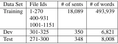
Several previous studies on Chinese parsing evaluate their parsers on the CTB version 5 (CTB5), which has approx-imately half a million words. Data split of CTB5 in those experiments is given in Table 3. The performance of the Berkeley parser on this dataset is provided in the first two rows of Table 4. Row #1 is the result from (Petrov and Klein, 2007),4and Row #2 is the result when we re-trained their parser with CTB5. The results in the two rows are very similar, as they should be.
4Somehow there are two slightly different versions
Expt Data ≤40 words All sentences
id Set P/R/F F-score range P/R/F F-score range
CTB5: Data split as in Table 3
#1 (Petrov & Klein, 2007) 86.9/85.7/86.3 86.3 84.8/81.9/83.3 83.3 #2 Retrained parser 87.1/85.4/86.2 86.2 84.6/82.7/83.6 83.6
CTB5: 10-fold cross validation
#3 w/o reshuffling 82.8/80.1/81.4 78.7-84.1 81.6/78.7/80.1 77.2-82.5 #4 with reshuffling 83.9/81.2/82.5 81.7-83.4 82.2/79.3/80.7 80.0-81.9
CTB7: 10-fold cross validation
#5 w/o reshuffling 78.2/79.7/78.9 72.8-88.9 78.1/78.7/78.4 72.8-88.7 #6 with reshuffling 83.9/81.3/82.6 82.1-83.2 82.8/80.0/81.4 80.9-82.1
Table 4: Performance of the Berkeley parser on CTB5 and CTB7. The P/R/F numbers in each cell are labeled precision, recall, and f-score. For Row #3–#6, P/R/F are the averages of 10 runs and F-score range shows the lowest and highest f-scores among the 10 runs.
Data Set File Ids # of sents # of words Training 1-270 18,089 493,939
400-931 1001-1151
Dev 301-325 350 6,821
Test 271-300 348 8,008
Table 3: Standard data split of the CTB5
Given that CTB7 is more than twice the size of CTB5, one might expect that the Berkeley parser, or any parser, would perform better when trained on CTB7 than on CTB5. Since there is not a standard data split for CTB7, we ran 10-fold cross validation on CTB7 and reported the average of precision/recall/f-score and the range of f-scores for the 10 runs. The results are in Row #5, which, surprisingly, are much worse than Row #2 (e.g., the f-score is 0.783 vs. 0.862 for sentences with no more than 40 words).
The main reason for low performance on CTB7 is due to genre variation in CTB7. Notice that the f-scores for the 10 runs on CTB7 in Row #5 vary a lot, ranging from 0.728 to 0.889. This is because the 10 folds of CTB7 are created based on file ids, and in a particular run training and test data can come from very different genres. For instance, in the run where the test data is the last 10% of data of CTB7 according to file ids, most of the test data belongs to the web genre, whereas the training data are mainly from the other four genres. To reduce the effect of file ids on the makeup of the 10 folds, we randomly reshuffle the files before dividing them into 10 folds. Row #6 lists the results of cross validation with the new 10 folds; not only do the average precision/recall/f-score increase, but also there is less variation among the 10 runs.
While reshuffling improves the performance on CTB7 by a few percentage points, it is still lower than the re-sults on CTB5 as in Row #2. There are two reasons for that. First, the data split in Table 3 turns out to be an easy one for the parser: the test data are all from Xinhua News, so are the development data and most files in the training set. When we ran 10-fold cross validation on CTB5 with or without file reshuffling, the average performance of the
10 runs, as shown in Row #3 and #4 in Table 4, is much worse than Row #2. Second, CTB7 is more diverse than CTB5; not only does it have documents from five genres (whereas CTB5 has only two genres: newswire and mag-azine), but the documents in CTB7 also come from more sources. For instance, the newswire documents in CTB5 are from Xinhua News and Hong Kong News, where the newswire documents in CTB7 can also come from other sources such as Agence France Presse (AFP), China News Service, People’s Daily, and Guangming Daily. As a result, the performance on CTB7 is worse than CTB5 without file reshuffling (#5 vs. #3), and is about the same as CTB5 with reshuffling (#6 vs. #4).
To summarize, Table 4 demonstrates the significant im-pact of genre variation on parsing performance in two ways. First, more training data does not necessarily lead to better performance (e.g. #5 vs. #3). Second, different splits of training, development and test data could lead to very dif-ferent parsing results (e.g., #2 vs. #3, #5 vs. #6), especially when the corpus is very diverse.
5.2. Performance of NLP tools on CTB7
For this set of experiments, we divide the data for each genre in CTB7 into three sets: the first 20% as the test portion, the first 150K words of the remaining 80% as the training portion, and the rest of the remaining 80% which are not used here. Tables 5-7 show the results of running three NLP tools on the data set. In each table, a row corre-sponds to the genre of the training data, and each column corresponds to the genre of the test data. The cell shows the performance of the tool when trained on the training portion of the training genre, and tested on the test portion of the test genre. That results in a5×5matrix. For each column, the highest score is in bold. In addition to the ma-trix, we also add an All row, where the training data is the union of the training portion of all five genres.
bc bn mz nw web bc 93.9 88.0 81.8 85.7 85.5 bn 87.9 94.1 82.8 87.6 85.1 mz 86.8 87.7 91.6 88.2 85.7 nw 83.1 89.7 85.8 94.6 83.8 web 92.1 89.5 84.2 86.8 91.5
All 96.1 96.1 93.2 96.2 93.5
Table 5: Performance of the CRF word segmenter on the CTB7. The numbers are f-scores for all the words.
bc bn mz nw web
bc 92.2 87.4 81.8 86.1 86.3 bn 87.1 93.2 84.5 90.5 86.6 mz 84.3 87.0 91.5 88.1 84.1 nw 84.2 88.8 86.5 94.1 84.9 web 90.3 89.1 87.1 88.6 90.9
All 93.8 94.2 92.4 94.7 92.0
Table 6: Performance of the Stanford POS tagger on the CTB7. The numbers in the table are tagging accuracy.
numbers in different columns, we can see that the NLP tools perform better on some genres (e.g., mz and web) than other genres (e.g.,bn and nw), for both in-domain and cross-domain settings, implying some genres are easier than other genres for these NLP tools. Third, from each matrix we can define the closeness of genres according to the performance of the NLP tool; that is, given test data in genre G1 and training data in genre G2 or G3, we say that G2 is closer to G1 than G3 is to G1 if the performance in cell (G2, G1) is better than the one in cell (G3, G1). For example, the first column in Table 5 indicates that web is closer to bc than nw. While all these observations are not surprising, what is interesting is that, although we using three tools, devel-oped by three institutes for three very different tasks, the rankings of genre closeness are very similar. For instance, for the test data in bc, the ranking of the training genres based on the word segmentation performance is the same as the ones based on POS tagging or parsing. In addition, if we rank genre difficulty based on system performance, the rankings are very similar for all three tasks, with nw and bn considered easier than the other three genres. Furthermore, ranking of genre closeness and ranking of genre difficulty
bc bn mz nw web
bc 74.9 68.2 61.9 64.7 69.5 bn 69.5 81.8 68.3 73.8 70.7 mz 66.2 70.3 76.6 70.5 69.4 nw 63.2 72.8 69.8 81.7 68.0 web 72.8 71.9 70.2 70.0 76.0
All 77.7 82.8 79.0 83.8 76.1
Table 7: Performance of Berkeley’s parser on the CTB7. The numbers in the table are labeled f-scores for sentences with no more than 40 words.
bc bn mz nw web
bc 8.88 17.91 24.21 17.92 17.14 bn 11.59 8.23 19.92 12.05 15.29 mz 13.60 16.83 10.44 15.66 16.31 nw 14.83 15.28 19.57 7.96 16.92 web 8.57 14.31 17.15 14.32 9.53
All 3.36 4.18 6.29 4.14 5.41
Table 8: OOV rates of the test data (i.e., the percentage of word tokens in the test data that do not appear in the training data). The lowest rate in each column is in bold.
are also consistent with the ranking based on the OOV rates in Table 8, where low OOV rates correspond to closeness in genres and higher performances for NLP tools. This re-sult implies that some properties of the corpora such as the OOV rate could be used as a cue to measure genre closeness or predict performance of NLP tools.
5.3. Prediction results on CTB7
For prediction experiments, we first divide the data in each genre into three portions: 20% as test data (Set3), 150k-words of the remaining 80% as training data for NLP tools (Set1), and the next one thousand sentences as training data for the predictor (Set2).5 For all the experiments, the chunk size was empirically set to be 10 sentences, which means that Set2 corresponds to 100 training instances for the pre-dictor. For these experiments, we did not use bc because af-ter putting aside 20% for Set3 and 150 thousand words for Set3, there are only 217 sentences left, which is too small for training the predictor.
Next we train a predictor for each genre pair and com-pare the predicted scores with the real scores. Section 4.2. described four groups of features: raw text features (F1), word-based features (F2), POS-tag-based features (F3), and parse-tree-based features (F4).
• For the three NLP tasks, F1 is always available as it depends on only the raw text; the availability of F2-F4 to the predictor varies from task to task.
• For word segmentation prediction, F2 is calculated from the output of the CFG segmenter for chunks in Set2 and Set3. For POS tagging and parsing, F2 is calculated from the gold standard of word boundary in Set2 and Set3 because both the tagger/parser and their predictor assume that the input text is segmented correctly.
• For POS tagging prediction, features in F3 are ex-tracted from the output of the Stanford tagger. • For parsing prediction, because the input to the
Berke-ley parser is a word segmented sentence with no POS tags, both F3 and F4 features are extracted from the output of the Berkeley parser. For the feature that com-pares two parse trees of the same sentence, the Stan-ford parser is used to process sentences in Set2 and Set3.
5
An example of the prediction matrix is given in Table 9, which is for POS tagging prediction with features in Group F1, F2, and F3. Features in F3 are calculated from the output of the Stanford tagger, not from the gold standard, because the gold standard for Set3 should be used only to evaluate the predictor, not to be used as part of input to the predictor. Each cell(i, j)has two numbers for genre pair (Gi, Gj): the first is the real accuracy of the POS tagger
when the tagger is trained on Set1 ofGiand tested on Set3
ofGj; the second number is the predicted accuracy when
the POS tagger is trained on Set1 ofGi, and the predictor
is trained on Set2 ofGiand tested on Set3 ofGj.
bn mz nw web
bn 93.2/93.7 84.5/90.4 90.5/91.8 86.6/92.0 mz 87.0/89.0 91.5/91.1 88.1/89.9 84.1/89.5 nw 88.8/89.4 86.5/86.4 94.1/93.8 84.9/81.0 web 89.1/90.1 87.1/88.0 88.6/88.7 90.9/91.8
Table 9: POS tagging prediction results on CTB7 with F1+F2+F3 features. The row specifies the genre of the training data (Set1 and Set2) and the column specifies the genre of the test data (Set3). The two numbers in each cell are real tagging accuracy and the predicted accuracy, re-spectively.
Table 9 shows that the predictor works reasonably well, as the gap between the two numbers is less than two per-centage points for 12 out of the 16 cells. More formally, we use two metrics to evaluate a predictor: one is the average of the difference between real scores and predicted scores (AvgDiff), and the other is root mean square (RMS), as de-fined in Eq (2) and (3). Here,nis the number of cells in the matrix;scorer,iandscorep,iare the two numbers in theith
cell.
AvgDif f =
Pn
i=1|scorer,i−scorep,i|
n (2)
RM S=
rPn
i=1(scorer,i−scorep,i)2
n (3)
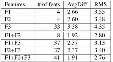
Tables 10-12 show the results of prediction with different feature combinations. There are several observations. First, among the three tasks, the prediction for word segmentation is the worst partly because, compared to POS tagging and parsing, there is less information available to the predictor. Second, more features normally lead to better performance, as illustrated by many feature combinations in the three ta-bles, but there are exceptions as shown in Table 12 for the feature combinations that include F4. Third, compared to other features which require more information present in the input, simple features such as the ones in F1 work pretty well for all three tasks, indicating that the raw text itself in-cludes a lot of information for performance prediction.
6.
Conclusion
To measure the effect of genre variation on NLP systems, we have run two sets of experiments. First, we compare the performance of the Berkeley parser on CTB5 and CTB7,
Features Feature # AvgDiff RMS
F1: raw text features
DLG-based score 1 4.97 5.39
OOV chars 1 6.07 6.90
Info Gain chars 1 7.52 8.40
All features in F1 4 5.26 5.66
F2: word-based features
OOV words 1 4.97 5.87
Info Gain words 1 6.80 7.76
word leng 1 6.79 7.72
All features in F2 4 5.19 5.96
All features in F1 + F2 8 5.10 5.68
Table 10: Word segmentation prediction results on the CTB7. F1: raw text features, F2: word-based features. F2 features are collected from the output of the CRF seg-menter.
Features # of feats AvgDiff RMS
F1 4 2.66 3.55
F2 4 2.60 3.48
F3 33 3.38 4.35
F1+F2 8 1.92 2.80
F1+F3 37 2.37 3.13
F2+F3 37 2.37 3.40
F1+F2+F3 41 1.91 2.76
Table 11: POS tagging prediction results on the CTB7. F1: raw text features, F2: word-based features, F3: POS-tag-based features. F3 features are collected from the output of the Stanford POS tagger.
and show that more training data does not necessarily lead to better performance. Second, we evaluate three NLP sys-tems with all the genre pairs in CTB7 and show that genre variation affects system performance significantly. While it is not surprising that NLP systems perform the best when the training and test data come from the same genre, what is interesting is, when we rank genres based on how close they are to a particular test genre or how well an NLP sys-tem performs on the genres, the rankings are very similar
Features # of feats AvgDiff RMS
F1 4 4.07 4.60
F2 4 4.88 5.89
F3 33 4.27 5.19
F4 29 3.27 3.78
F1+F2 8 3.72 4.76
F1+F4 33 3.60 4.50
F2+F4 33 3.52 4.45
F1+F2+F3 41 2.70 3.79
F1+F2+F3+F4 70 3.40 4.19
no matter which NLP system we use. This implies that these rankings are more likely to result from some inherent properties of the genres than from properties of a particular NLP system.
In addition to studying genre variation, we also build a predictor for the three NLP systems and report experimen-tal results with different feature combinations. Among the three systems, the prediction for the Stanford POS tagger is the best, followed by the Berkeley parser, and followed by the CRF word segmenter.
As mentioned in Section 2.1., many important questions about genre variation (such as how to measure similar-ity between genres and what exactly causes performance degradation of NLP systems when tested on a different genre) have not been studied a lot in the NLP field. We plan to address these questions in the future. For perfor-mance prediction, we will experiment with various feature selection methods to find a good feature combination for a given NLP system.
7.
Acknowledgements
The work is partly supported by the Intelligence Advanced Research Projects Activity (IARPA) via Department of In-terior National Business Center (DoI/NBC) contract num-ber D11PC20153. The U.S. Government is authorized to reproduce and distribute reprints for Governmental pur-poses notwithstanding any copyright annotation thereon. The views and conclusions contained herein are those of the authors and should not be interpreted as necessarily rep-resenting the official policies or endorsements, either ex-pressed or implied, of IARPA, DoI/NBC, or the U.S. Gov-ernment, We would also like to thank three anonymous re-viewers for very helpful comments.
8.
References
Joshua Albrecht and Rebecca Hwa. 2007. Regression for sentence-level MT evaluation with pseudo references. In Proceedings of ACL, pages 296–303, Prague, Czech Re-public.
Hal Daume. 2007. Frustratingly easy domain adaptation. In Proceedings of ACL-2007, pages 256–263, Prague, Czech Republic.
Aidan Finn and Nicholas Kushmerick. 2003. Learning to classify documents according to genre: Special topic section on computational analysis of style. the Amer-ican Society for Information Science and Technology, 57(11):1506–1518.
Daniel Gildea. 2001. Corpus variation and parser perfor-mance. In Proceedings of EMNLP, pages 167–202. Chunyu Kit and Yorick Wilks. 1999. Unsupervised
learn-ing of word boundary with description length gain. In Proceedings of CoNLL-1999, pages 1–6.
Dan Klein and Christopher D. Manning. 2003. Fast ex-act inference with a fex-actored model for natural language parsing. In Proceedings of Advances in Neural Informa-tion Processing Systems (NIPS), pages 3–10, Cambridge, MA.
J. Lafferty, A. McCallum, and F. Pereira. 2001. Condi-tional random fields: Probabilistic models for
segment-ing and labelsegment-ing sequence data. In Proc. of the 18th In-ternational Conference on Machine Learning (ICML), pages 282–289.
Mitch Marcus, Mary Ann Marcinkiewicz, and Beatrice Santorini. 1993. Building a large annotated corpus of English: the Penn Treebank. Computational Linguistics, 19(2):313–330.
David McClosky, Eugene Charniak, and Mark Johnson. 2006. Effective self-training for parsing. In Proc. of NAACL-HLT, pages 152–159.
David McClosky, Eugene Charniak, and Mark Johnson. 2010. Automatic domain adaptation for parsing. In Pro-ceedings of HLT-NAACL, pages 28–36.
Robert Moore and William Lewis. 2010. Intelligent selec-tion of language model training data. In Proceedings of ACL, pages 220–224.
Kishore Papineni, Salim Roukos, Todd Ward, and Wei-Jing Zhu. 2002. BLEU: a Method for Automatic Evaluation of Machine Translation. In Proceedings of ACL, pages 311–318.
Slav Petrov and Dan Klein. 2007. Improved inference for unlexicalized parsing. In Proceedings of HLT-NAACL, pages 404–411.
Barbara Plank and Gertjan van Noord. 2011. Effective measures of domain similarity for parsing. In Proceed-ings of ACL, pages 1566–1576, Portland, Oregon, USA. R. Prasad, N. Dinesh, A. Lee, E. Miltsakaki, L. Robaldo,
A. Joshi, and B. Webber. 2008. The Penn discourse tree-bank 2.0. In Proceedings of LREC, pages 2961–2968. Sujith Ravi, Kevin Knight, and Radu Soricut. 2008.
Au-tomatic prediction of parser accuracy. In Proceedings of EMNLP, pages 887–896, Honolulu, Hawaii.
Brian Roark and M. Bacchiani. 2003. Supervised and un-supervised PCFG adaptation to novel domains. In Pro-ceedings of NAACL-HLT, pages 126–133.
Douglas Roland and Daniel Jurafsky. 1998. How verb sub-categorization frequencies are affected by corpus choice. In Proceedings of COLING, pages 1122–1128.
K. Toutanova, Dan Klein, Christopher D. Manning, and Yoram Singer. 2003. Feature-rich part-of-speech tag-ging with a cyclic dependency network. In Proceedings of HLT-NAACL 2003, pages 252–259.
Bonnie Webber. 2009. Genre distinctions for discourse in the penn TreeBank. In Proceedings of ACL-IJCNLP, pages 674–682.
Fei Xia, Martha Palmer, Nianwen Xue, Mary Ellen Okurowski, John Kovarik, Shizhe Huang, Tony Kroch, and Mitchell Marcus. 2000. Developing Guidelines and Ensuring Consistency for Chinese Text Annotation. In Proceedings of LREC, Athens, Greece.
Nianwen Xue. 2003. Chinese Word Segmentation as Char-acter Tagging. International Journal of Computational Linguistics and Chinese Language Processing, 8(1):29– 48.