!∀#!!!∃
!%&∋(
)∗++ , ,−+.%(.+
Software Defect Association Mining
and Defect Correction Effort Prediction
Qinbao Song, Martin Shepperd, Michelle Cartwright, and Carolyn Mair
Abstract—Much current software defect prediction work focuses on the number of defects remaining in a software system. In this paper, we present association rule mining based methods to predict defect associations and defect correction effort. This is to help developers detect software defects and assist project managers in allocating testing resources more effectively. We applied the proposed methods to the SEL defect data consisting of more than 200 projects over more than 15 years. The results show that, for defect association prediction, the accuracy is very high and the false-negative rate is very low. Likewise, for the defect correction effort prediction, the accuracy for both defect isolation effort prediction and defect correction effort prediction are also high. We compared the defect correction effort prediction method with other types of methods—PART, C4.5, and Naı¨ve Bayes—and show that accuracy has been improved by at least 23 percent. We also evaluated the impact of support and confidence levels on prediction accuracy, false-negative rate, false-positive rate, and the number of rules. We found that higher support and confidence levels may not result in higher prediction accuracy, and a sufficient number of rules is a precondition for high prediction accuracy.
Index Terms—Software defect prediction, defect association, defect isolation effort, defect correction effort.
æ
1
INTRODUCTION
T
HEsuccess of a software system depends not only on cost and schedule, but also on quality. Among many software quality characteristics, residual defects has become thede factoindustry standard [12]. Therefore, the prediction of software defects, i.e., deviations from specifications or expectations which might lead to failures in operation [11], has been an important research topic in the field of software engineering for more than 30 years. Clearly, they are a proxy for reliability, but, unfortunately, reliability is extremely difficult to assess prior to full deployment.Current defect prediction work focuses on estimating the number of defects remaining in software systems with code metrics, inspection data, and process-quality data by statistical approaches [7], [18], [9], capture-recapture (CR) models [27], [21], [6], [10], and detection profile methods (DPM) [28].
The prediction result, which is the number of defects remaining in a software system, can be used as an important measure for the software developer [16], and can be used to control the software process (i.e., decide whether to schedule further inspections or pass the soft-ware artifacts to the next development step [19]) and gauge the likely delivered quality of a software system [11]. In contrast, Bhandari et al. [4], [5] propose that the defects found during production are a manifestation of process
deficiencies, so they present a case study of the use of a defect based method for software in-process improvement. In particular, they use an attribute-focusing (AF) method [3] to discover associations among defect attributes such as defect type, source, phase introduced, phase found, component, impact, etc. By finding out the event that could have led to the associations, they identify a process problem and implement a corrective action. This can lead a project team to improve its process during development. We restrict our work to the predictions of defect (type) associations and corresponding defect correction effort. This is to help answer the following questions:
1. For the given defect(s), what other defect(s) may co-occur?
2. In order to correct the defect(s), how much effort will be consumed?
We use defect type data to predict software defect associations that are the relations among different defect types such as: If defectsaandboccur, then defectcalso will occur. This is formally written as a^b)c. The defect associations can be used for three purposes:
First, find as many related defects as possible to the detected defect(s) and, consequently, make more-effective corrections to the software. For example, consider the situation where we have classes of defect a, b, andc and suppose the rule a^b)c has been obtained from a historical data set, and the defects of class a and b have been detected occurring together, but no defect of class c
has yet been discovered. The rule indicates that a defect of classcis likely to have occurred as well and indicates that we should check the corresponding software artifact to see whether or not such a defect really exists. If the result is positive, the search can be continued so, if rulea^b^c)d
holds as well, we can do the same thing for defect d. We . Q. Song is with the Department of Computer Science and Technology,
Xi’an Jiaotong University, 28 Xian-Ning West Rd., Xi’an, Shaanxi, 710049 China. E-mail: [email protected].
. M. Shepperd, M. Cartwright, and C. Mair are with the School of
Information Science, Computing, and Mathematics, Brunel University, Uxbridge, UB8 3PH UK.
E-mail: {martin.shepperd, michelle.cartwright, carolyn.mair}@brunel.ac.uk. Manuscript received 9 Dec. 2004, revised 10 Oct. 2005; accepted 2 Dec. 2005; published online 15 Feb. 2006.
Recommended for acceptance by R. Lutz.
For information on obtaining reprints of this article, please send e-mail to: [email protected], and reference IEEECS Log Number TSE-0276-1204.
believe this may be useful as it permits more-directed testing and more-effective use of limited testing resources.
Second, help evaluate reviewers’ results during an inspection. For example, if rule a^b)c holds but a reviewer has only found defectsaandb, it is possible that (s)he missed defect c. Thus, a recommendation might be that his/her work should be reinspected for completeness. Third, to assist managers in improving the software process through analysis of the reasons some defects frequently occur together. If the analysis leads to the identification of a process problem, managers have to come up with a corrective action.
At the same time, for each of the associated defects, we also predict the likely effort required to isolate and correct it. This can be used to help project managers improve control of project schedules.
Both of our defect association prediction and defect correction effort prediction methods are based on the association rule mining method which was first explored by Agrawal et al. [1]. Association rule mining aims to discover the patterns of co-occurrences of the attributes in a database. However, it must be stressed that associations do not imply causality. An association rule is an expression
A ) C, whereA (Antecedent) andC (Consequent) are sets of items. The meaning of such rules is quite intuitive: Given a databaseDof transactions, where each transactionT 2 D
is a set of items, A ) C expresses that whenever a transaction T contains A, then T also contains C with a specified confidence. The rule confidence is defined as the percentage of transactions containing C in addition to A
with regard to the overall number of transactions containingA.
The idea of mining association rules originates from the analysis of market-basket data where rules like “customers who buy productsp1 andp2will also buy productp3 with probability c percent” are extracted. Their direct applic-ability to business problems together with their inherent understandability make association rule mining a popular data mining method. However, it is clear that association rule mining is not restricted to dependency analysis in the context of retail applications, but can successfully be applied to a wide range of business and science problems. Although association rule mining aims to discover the co-occurring patterns of the attributes in databases, it has been shown that association rule mining based classifica-tion—associative classification—frequently has higher clas-sification accuracy than other clasclas-sification methods. The underlying reason is that these methods use heuristic/ greedy search techniques to build classifiers; they induce a representative subset of rules. However, as association rule mining explores high-confidence associations among multi-ple variables, it may overcome some constraints introduced by other techniques, e.g., decision-tree induction methods that examine one variable at a time. Thus, associative classification takes the most effective rule(s) from among all the rules mined for classification.
Extensive performance studies have also shown that associative classification frequently generates better accu-racy than state-of-the-art classification methods. Ali et al. [2] use association rule mining to do a partial
classification in the context of very large numbers of class attributes, when most attribute values are missing, or the class distribution is highly skewed and the user is interested in understanding the low-frequency classes. Liu et al. [17] and Yin and Han [30] integrate classification and association rule mining to build a classifier; the former method prunes rules using both minimum support and pessimistic estimation. Wang et al. [26] proposed a general method for turning an arbitrary set of association rules into a classifier. Dong et al. [8] combined several association rules to classify a new case, which partially addressed the low support of classification rules because a combined rule has a lower support. Wang et al. [25] used multilevel association rules to build hierarchical classifiers where both the class space and the feature space are organized into a taxonomy. Association rule mining based methods have also been used in the prediction of WWW caching and prefetching [29], outer membrane proteins [23], and software source-code changes [31], [32]. The successful use of association rule mining in various fields motivates us to apply it to the software defect data set.
The rest of the paper is organized as follows: In Section 2, we describe the approach used by the study. In Section 3, we present the specific defect association and defect-correction effort prediction methods. In Section 4, we present our experimental results. Finally, in Section 5, we summarize our work and findings.
2
RESEARCH
METHOD
2.1 General MethodThe objective of the study is to discover software defect associations from historical software engineering data sets, and help determine whether or not a defect(s) is accom-panied by other defect(s). If so, we attempt to determine what these defects are and how much effort might be expected to be used when we correct them. Finally, we aim to help detect software defects and effectively improve software control.
For this purpose, first, we preprocessed the NASA SEL data set (see the following section for details), and obtained three data sets: the defect data set, the defect isolation effort data set, and the defect correction effort data set. Then, for each of these data sets, we randomly extracted five pairs of training and test data sets as the basis of the research. After that, we used association rule mining based methods to discover defect associations and the patterns between a defect and the corresponding defect isolation/correction effort. Finally, we predicted the defect(s) attached to the given defect(s) and the effort used to correct each of these defects. We also compared the results with alternative methods where applicable.
2.2 Data Source and Data Extraction
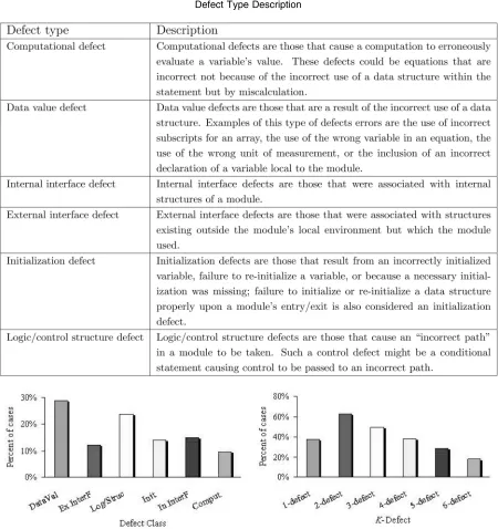
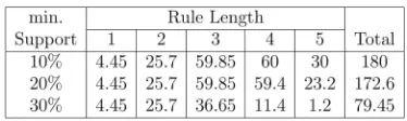
The SEL Data is a database consisting of 15 tables that provide data on the projects’ software characteristics (over-all and at a component level), changes and errors during (over-all phases of development, and effort and computer resources used. In the SEL Data, the defects are divided into six types, Table 1 contains the details. See [15] for further information. In addition, the effort used to correct defects falls into four categories: One Hour or Less, One Hour to One Day, One Day to Three Days, and More Than Three Days.
For the purpose of defect association prediction, we used SQL to extract defect data from different tables of the SEL data and obtained the basic defect data set. The defect data is very simple, and consists of defect types and the corresponding dates on which the need for change was determined. Then, we followed the sliding window
approach, that is, two subsequent defectsa andb are part of one transaction if they are at most one day apart and belong to the same project, to infer the transactions needed for the association rule mining. Fig. 11 contains summary information. We would like to clarify that while we set the size of the sliding window to one day in this analysis, it does not imply that we are limited to this value and it could be set to any other time interval thought appropriate. Moreover, placing defects into one transaction according to the selected sliding window just means they co-occur during the given time window, it does not imply they
1. The notationk-defect means that kdefects occurred together in a transaction.
TABLE 1 Defect Type Description
must be dependent. However, if the placement of defects is coincidental they tend not to form association rules.
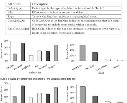
For the purpose of defect correction effort prediction, we also used SQL to extract defect data and the corresponding isolation and correction effort data from SEL data and obtained two further data sets: the defect isolation effort data set and the defect correction effort data set. Both consist of five attributes (see Table 2 for details). Fig. 2 and Fig. 3 provide the corresponding summary information.
For both the defect association and defect correction effort predictions, the data setDis randomly split into five mutually exclusive subsetsD1,D2,. . ., andD5of equal size, and[5
i¼1Di¼ D. We usedD Dt2ðt¼ f1;2;. . .;5gÞ, andDt as training sets and test sets, respectively.
2.3 Analysis Approach
We use the five-fold cross-validation method as the overall analysis approach. That is, for eachDof the defect data set,
the defect isolation effort data set, and the defect correction effort data set, the inducer is trained and tested a total of five times. Each timet2 f1;2;. . .;5g, it is trained onD Dt and tested onDt.
We use the association rule mining method to learn rules from the training data sets. For defect association predic-tion, the rule learning is straightforward, while for defect correction effort prediction, it is more complicated because the consequent of a rule has to be defect correction effort. Considering the target of association rule mining is not predetermined and classification rule mining has only one predetermined target, the class, we integrate these two techniques to learn defect correction effort prediction rules by focusing on a special subset of association rules whose consequents are restricted to the special attribute, the effort. Once we obtain the rules, we rank them, and use them to predict the defect associations and defect correction effort with the corresponding test data sets. The predictions of defect associations and defect correction effort are both
2. The notationD Dtmeans setDminus setDt.
TABLE 2
Defect Effort Data Description
Fig. 2. Distribution of cases by defect type and effort for the isolation effort data set.
based on the length-first (in terms of the number of items in a rule) strategy (see Section 3.2 for details).
To our knowledge, there is no work on software defect association prediction and there is no other method that can be used for this purpose. Therefore, we are unable to directly compare our defect association prediction method with other studies. As the defect correction effort is represented in the form of categorical values and there are some attributes to characterize it, it can be viewed as a classification problem. This allows us to compare our defect correction prediction method with three different types of methods. These methods are the Bayesian rule of condi-tional probability-based method, Naı¨ve Bayes [13], the well-known trees-based method, C4.5 [20], and the simple and effective rules-based method, PART [14].
3
RULE
DISCOVERY AND
DEFECT/EFFORT
PREDICTION
In this section, we first introduce the basic concepts of association rule mining. Then, we present the rule-ranking strategy used for the purpose of defect association and defect correction effort predictions. After that, we respec-tively give the methods of defect association prediction and defect correction effort prediction based on the association rule mining method.
3.1 Association Rule Discovery
Association rule mining searches for interesting relation-ships, e.g., frequent patterns, associations, correlations, or potential causal structures, among sets of objects in databases or other information repositories. The approach is data rather than hypothesis driven. The interestingness of an association rule is measured by both support and confidence, which respectively reflect the usefulness and certainty of the rule. It must be stressed that even rules that discover with high levels of support (or relevance) and high confidence do not necessarily imply causality. However, such rules would obviously stimulate further research through the postulation of models that can be empirically evaluated.
LetI ¼ fI1;I2;. . .;Imgbe a set of attribute values, called items. A setA Iis called an item set. Let a databaseDbe a multiset of I. Each T 2 D is called a transaction. An association rule is an expression A ) C, where A I,
C I, and ATC ¼. We refer to A as the antecedent of the rule, andCas the consequent of the rule. The ruleA ) C
has supportSuppðA ) CÞinD, where thesupportis defined as SuppðA ) CÞ ¼SuppðASCÞ. That means SuppðA ) CÞ
percent of the transactions in D contain ASC, and
SuppðAÞ ¼ jfT 2 DjA T gj=jDjis the support ofAthat is the fraction of transactionsT supporting an item setAwith respect to databaseD. The number of transactions required for an item set to satisfy minimum support is referred to as theminimum support count. A transactionT 2 Dsupports an item setA I ifA T holds. The rule A ) Cholds inD
with confidence ConfðA ) CÞ, where the confidence is defined as ConfðA ) CÞ ¼SuppðASCÞ=SuppðAÞ. That means ConfðA ) CÞ percent of the transactions in Dthat containAalso containC. The confidence is a measure of the
rule’s strength or certainty while the support corresponds to statistical significance or usefulness.
Association rule mining generates all association rules that have a support greater than minimum support
min:SuppðA ) CÞ, in the database, i.e., the rules are frequent. The rules must also have confidence greater than minimum confidencemin:ConfðA ) CÞ, i.e., the rules are strong. The process of association rule mining consists of these two steps: 1) Find all frequent item sets, where each
ASC of these item sets must be at least as frequently supported as the minimum support count. 2) Generate strong rules from the discovered frequent item sets, where each A ) C of these rules must satisfy min:SuppðA ) CÞ
andmin:ConfðA ) CÞ. 3.2 Rule-Ranking Strategy
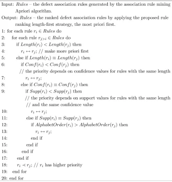
Before prediction, we rank the discovered rules according to the length-first strategy. The length-first strategy was used for two reasons. First, for the defect association prediction, the length-first strategy enables us to find out as many defects as possible that coincide with known defect(s), thus preventing errors due to incomplete dis-covery of defect associations. Second, for the defect correction effort prediction, the length-first strategy enables us to obtain more-accurate rules, thus improving the effort-prediction accuracy.
Specifically, the length-first rule-ranking strategy is as follows:
1. Rank rules according to their length. The longer the rules, the higher the priority.
2. If two rules have the same length, rank them according to their confidence values. The greater the confidence values, the higher the priority. The more-confident rules have more predictive power in terms of accuracy; thus, they should have higher priority.
3. If two rules have the same confidence values, rank them according to their support values. The higher the support values, the higher the priority. The rules with higher support value are more statistically significant, so they should have higher priority. 4. If two rules have the same support value, rank them
in alphabetical order.
The algorithmic description of the strategy is shown in Fig. 4.
3.3 Defect Association Prediction
association rule mining method is able to find rules like
Defectfag )DefectfNULLg, which means defect a
occurred independently.
The next step is to predict whether or not ak-defectwill occur with others. The prediction begins by ranking the discovered rules according to the strategy presented in Section 3.2. Then, for thek-defect, we scan the rules one by one and identify the rule whose antecedent contains the
k-defect. After that, we merge the consequent of the corresponding rule with the k-defect and generate a ðkþ1Þ-defect. For theðkþ1Þ-defect, we repeat the process until there are no rules available, the fðkþnÞ-defectg fk-defectgis the defect(s) which occurred with thek-defect. Fig. 5 contains an algorithmic description of the procedure. The measures used to evaluate the defect association prediction method are prediction accuracy, false-negative rate, and false-positive rate, which are defined as follows: LetGbe a given original defect set,Rbe the real defect set, andPbe the predicted defect set. The predictionaccuracyof
P is defined as:
AccuracyðPÞ ¼jðR GÞ \ ðP GÞj
jR Gj ; ð1Þ
where, if G R PorR P,AccuracyðPÞ ¼1.
We use the false-negative rate and false-positive rate to present the prediction error of defect associations. The false-negative rate F N denotes how many defects that are not predicted to occur along with the given set G but actually do, and is defined as follows:
F N ðPÞ ¼jR R \ Pj
jR Gj ; ð2Þ
where, ifG R PorR P,F N ðPÞ ¼0.
Thefalse-positive rateF P denotes how many defects are predicted to occur along with the given setGbut actually do not. It is defined as follows:
F PðPÞ ¼jP R \ Pj
jR Gj ; ð3Þ
where, ifG R PorR P,F PðPÞ ¼0.
3.4 Defect Correction Effort Prediction
Because the intent of defect correction effort3prediction is predetermined and the association rule mining has no special goal, the association rule mining based discovery of defect correction effort prediction rules is not straightforward. For Fig. 4. Rule-ranking (RR) strategy.
the purpose of defect correction effort prediction, we used the constraint-based association rule mining method [24]. Specifically, the procedure of association rule mining was adapted as follows:
1. Compute the frequent item sets that occur together in the training data set at least as frequently as a predeterminedmin:Supp. The item sets mined must also contain the effort labels.
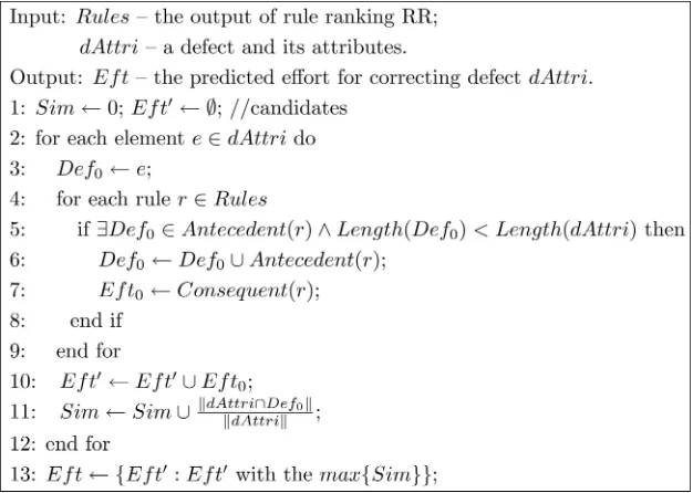
2. Generate association rules from the frequent item sets, where the consequent of the rules is the effort. In addition to the min:Supp threshold, these rules must also satisfy a minimum confidencemin:Conf. For the algorithmic description of the constraint-based association rule mining procedure, we refer readers to [24]. Once the rules are obtained, we rank them according to the approach presented in Section 3.2. Then, for each element of the given defect and its attributes, we scan the rules one by one and identify the rule whose antecedent contains the element. After that, we merge the antecedent of the corresponding rule with the element, generate an element set, and obtain the corresponding effort. For the element set, we continue the scan until no more rules fit. At
this point, we have obtained the most likely candidate effort and the corresponding similarity for the element. We repeat the process until all the elements of the given defect and its attributes have been checked. Finally, we compare the similarities of all the candidates; the most similar candidate’s effort is the defect correction effort for the given defect and its attributes. Fig. 6 is the algorithmic description which contains the details of the procedure.
As the defect correction effort is represented in catego-rical values and there are some attributes characterizing it, it can be viewed as a classification problem. Hence, we use the normal classification accuracy measure to evaluate the defect correction effort prediction method and the other three methods.
4
EXPERIMENTAL
RESULTS
In this section, we present the experimental results for the defect data set, the defect isolation effort data set, and the defect correction effort data set with different minimum-support thresholds and different minimum-confidence thresholds for association rule mining based defect associa-tion and defect correcassocia-tion effort predicassocia-tions. We also Fig. 5. Defect association prediction procedure.
compared the proposed methods with the other three methods if applicable. As five training and test sets were used, for each of the defect data set, the defect isolation effort data set, and the defect correction effort data set, we let the average accuracy of the corresponding five test sets be the final result.
4.1 Defect Association Prediction
4.1.1 Defect Association Rules
When mining defect association rules, we applied three values for minimum support (10, 20, and 30 percent) and four minimum confidence values (30, 40, 50, and 60 percent). This means a total of 12 cases were considered. At the same time, these 12 cases were applied to the five training data sets, which were derived from the defect data set by using the method presented in Section 2.2. This resulted in a total of 60 sets of rules, which consist of more than 1,000 rules. For this reason, we do not list them all (!), but instead present their typical forms and the statistical analysis of the results.
The typical forms of the defect association rules are listed below:
. DefectfDataV alueg
)DefectfNullg@ð32:5%;79:9%Þ.
. DefectfEx:Interfaceg
)DefectfComput:g@ð39:0%;69:5%Þ.
. DefectfComput:g ^DefectfIni:g
)DefectfEx:Interfaceg@ð34:3%;75:1%Þ.
. DefectfIn:Interfaceg ^DefectfIni:g ^ DefectfDataV alueg
)DefectfLogi:Strucg@ð35:4%;94:8%Þ.
. DefectfComput:g ^DefectfIni:g ^ DefectfLogi:Strucg
^ DefectfDataV alueg
)DefectfIn:Interfaceg@ð31:4%;88:1%Þ.
The first is a one-defect rule, which means that defect
DataV alueoccurred independently in 32.5 percent of cases in the defect data set and, when occurring, it is independent with a probability of 79.9 percent. The second is a two-defect rule, which means these two two-defects can co-occur. This rule shows that 39 percent of the cases in the defect data set contain both defects Ex:Interface and Comput:,
and 69.5 percent of the cases in the defect data set that contain defectsEx:Interfacealso contain defectComput:It reveals that defect Comput: can co-occur with defect
Ex:Interface with a significance of 39 percent and a certainty of 69.5 percent. The third is a three-defect rule, which means these three defects can co-occur. This rule shows that 34.3 percent of the cases in the defect data set contain defects Comput:, Ini:, and Ex:Interface, and 75.1 percent of the cases in the defect data set that contain defectsComput:andIni:also contain defectEx:Interface. It reveals that defectEx:Interfacecan co-occur with defects
Comput: and Ini: with a significance of 34.3 percent and a certainty of 75.1 percent. The fourth is a four-defect rule, which reveals that defect Logi:Struc can co-occur with defects In:Interface, Ini:, and DataV alue with a significance of 35.4 percent and a certainty of 94.8 percent. The fifth is a five-defect rule, which reveals that defect In:Interfacec can co-occur with defects Comput:,
Ini:, Logi:Struc, and DataV alue with a significance of 31.4 percent and a certainty of 88.1 percent.
Fig. 7 is the distribution of defect association rules by minimum support (min:Supp) for all five training data sets. We observe that the overall behaviors of the training data sets are very similar except for the data setD1. Specifically, for each data set, the average number of rules decreases as the min:Supp increases from 10 percent through 20 to 30 percent, and the decrease is very sharp whenmin:Supp
exceeds 20 percent.
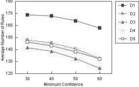
Fig. 8 is the distribution of defect association rules by minimum confidence (min:Conf) again for all five training data sets. We observe that for each data set, the average number of rules decreases asmin:Conf increases from 30 percent through 40 percent and 50 to 60 percent, but the average number of rules for data setD1is greater than other data sets at each confidence point.
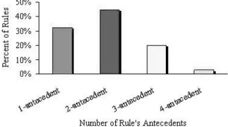
Fig. 9 is the distribution of defect association rules by rule length. Comparing it with Fig. 1, we observe that these two distributions are dissimilar, especially for one-defect and two-defect. This is because there are only six types of defects. Thus, for one-defect, six rules can cover all cases and, for two-defect, the combinations of any two of six defects are also relative smaller, moreover, some defects may never occur together.
Fig. 7. Distribution of defect association rules byMin:Suppfor the five defect data sets.
4.1.2 Defect Association Prediction Results
Table 3 contains the defect association prediction results with min:Supp¼20% and min:Conf¼30%. We observe that the defect association prediction accuracy is very high and the false negative rateF N is very low. These are both desirable. The smaller the false negative rate F N, the smaller the possibility that the defect associations are not identified. On the other hand, the false positive rate F Pis rather high, but this guarantees that we can find more defects. However, the cost is increased testing effort.
Table 4 and Table 5 show the results of the impact of
min:Supp and min:Conf on the defect association predic-tion accuracy, respectively. Table 4 shows that both the defect association prediction accuracy and the false-positive rateF Pdecrease, but the false-negative rateF N increases as min:Supp increases from 10 to 30 percent. The defect association prediction accuracy withmin:Supp¼10%is the same as min:Supp¼20% except the F P of the former is greater than the latter. This means decreasingmin:Supphas no further impact upon the prediction accuracy. In contrast, it will increase the F P, which is something we wish to avoid.
Table 5 reveals that the defect association prediction accuracy decreases, but both F P and F N increase as
min:Conf increases from 30 to 60 percent. This means that
increasingmin:Conf cannot improve the prediction accu-racy further. In contrast, it will increase bothF PandF P.
The quality of defect association prediction depends on the rules, thus we also explored the impact ofmin:Suppand
min:Conf on the number of rules and further on the prediction accuracy. Table 6 and Table 7 show the results. We observe that the total number of rules with different length decreases asmin:Suppincreases from 10 to 30 per-cent. It seems thatmin:Supp affects long rules more than short ones butmin:Confaffects short rules more than long rules, although the total number of rules with different length decreases as min:Conf increases from 30 to 60 percent. In comparison with Table 3, we find that in order to obtain high prediction accuracy, a sufficient number of rules is a precondition.
4.2 Defect Isolation Effort Prediction
4.2.1 Defect Isolation Effort Prediction Rules
Again, we have 12 cases to consider (minimum support values of 10, 20, and 30 percent combined with minimum confidence values of 10, 20, 30, and 40 percent). These 12 cases are applied to the five training data sets, which were derived from the defect isolation data set by using the method presented in Section 2.2. Again, this yields a total of 60 sets of rules, which total more than 1,000 rules.
The typical forms of the defect isolation effort prediction rules are listed as follows:
Fig. 9. Distribution of defect association rules by rule length for the defect data set.
TABLE 3
Defect Association Prediction Accuracy
TABLE 4
Defect Association Prediction Accuracy with Different Minimum Supports
TABLE 5
Defect Association Prediction Accuracy with Different Minimum Confidences
TABLE 6
Number of Defect Association Prediction Rules by Rule Length with Different Minimum Supports
TABLE 7
. DefectfIni:g )EffortfOne Hour or Lessg
@ð15:3%;64:1%Þ
. DefectfComput:g ^AttrifT ypoErr¼Ng )EffortfOne Day to T hree Daysg @ð10:2%;10:5%Þ.
. DefectfLogic:Strug ^AttrifT ypoErr¼Ng ^AttrifOmisErr¼Yg
)EffortfOne Hour to One Dayg @ð15:4%;40:1%Þ.
. DefectfDataV alueg ^AttrifT ypoErr¼Ng ^AttrifOmisErr¼Ng ^ AttrifComisErr¼Yg )EffortfOne Hour or Lessg@ð10:6%;64:5%Þ. The first rule contains only one antecedent. It shows that for an initialization defect, no matter what attributes are attached, the effort used to isolate it is One Hour or Less with a significance of 15.3 percent and a certainty of 64.1 percent. The second rule shows that 10.2 percent of the cases in the defect isolation effort data set contain defect
Comput:, defect attributeT ypoErr¼N, and defect isolation effort One Day to Three Days, and 10.5 percent of the cases in the defect isolation effort data set that contain defects
Comput: and T ypoErr¼N also contain defect isolation effort One Day to Three Days. This means that if a computational defect was not caused by a typographical error, we can say the effort used to isolate it is One Day to
Three Days with a significance of 10.2 percent and a certainty of 10.5 percent. The third rule reveals that if a logical-structure defect was caused not by a typographical error but by an omission error, we can say the effort used to isolate it is One Hour to One Day with a significance of 15.4 percent and a certainty of 40.1 percent. The fourth rule reveals that if a data-value defect was caused neither by a typographical error nor by an omission error but by a commission error, we can say the effort used to isolate it is One Hour or Less with a significance of 10.6 percent and a certainty of 64.5 percent.
Fig. 10 is the distribution of defect isolation effort prediction rules by minimum supportmin:Suppfor all five training data sets. We observe that, for each data set, the average number of rules decreases as the minimum support
min:Supp increases from 10 percent through 20 to 30 percent, and the decrease is very sharp whenmin:Supp
exceeds 10 percent but is less than 20 percent.
Fig. 11 is the distribution of defect isolation effort prediction rules by minimum confidencemin:Conf for all the five training data sets. We observe that, for each data set, the average number of rules decreases as the minimum confidencemin:Conf increases from 10 percent through 20 and 30 percent to 40 percent, and the decrease is sharp whenmin:Conf exceeds 30 percent.
Fig. 12 is the distribution of defect isolation effort prediction rules by rule length. We observe that nearly half of the rules have two antecedents and more than 30 percent of rules have one antecedent. Thus, these rules constitute the main part of the rule set.
4.2.2 Defect Isolation Effort Prediction Results
Table 8 contains the defect isolation effort prediction results of four methods: association rule mining based method Fig. 10. Distribution of defect isolation effort prediction rules by
Min:Suppfor the five defect isolation effort data sets.
Fig. 11. Distribution of defect isolation effort prediction rules by Min:Conf for the five defect isolation effort data sets.
Fig. 12. Distribution of defect isolation effort prediction rules by rule length for the defect isolation effort data set.
TABLE 8
(withmin:Supp¼10%andmin:Conf¼10%), PART, C4.5, and Naı¨ve Bayes. We observe that the accuracy of the association rule mining based method is higher than the other three methods by at least 25 percent. This means for the purpose of predicting defect isolation effort, association rule mining substantially outperforms the Bayesian prob-ability, tree, and rule-based methods. The reason associa-tion rule mining based predicassocia-tion performs so much better than other methods is that it explores high confidence associations among multiple variables and discovers inter-esting rules, i.e., rules that are useful, strong, and significant. By contrast, the other methods use domain independent biases and heuristics to generate a small set of rules, which results in many interesting and useful rules remaining undiscovered.
Table 9 and Table 10 are the results of the impact of
min:Supp and min:Conf on the defect isolation effort prediction accuracy, respectively. Table 9 shows that the defect isolation effort prediction accuracy decreases as
min:Suppincreases from 10 to 30 percent, and the accuracy with min:Supp¼10% is just a little better than
min:Supp¼20%. This means decreasing min:Supp cannot greatly improve the prediction accuracy.
Table 10 shows that the defect isolation effort prediction accuracy decreases as min:Conf increases from 9 to 40 percent, and the accuracy withmin:Conf¼10%slightly higher than min:Conf¼20%. This means decreasing
min:Conf doesn’t greatly improve prediction accuracy. Table 11 and Table 12 are the results of the impact of
min:Suppandmin:Conf on the number of defect isolation effort prediction rules, respectively. We observe that the total number of rules with different length decreases as both
min:Supp and min:Conf increase. It seems that the conclusion that a sufficient number of rules is a precondi-tion for high predicprecondi-tion accuracy also works in the context of defect isolation effort prediction.
4.3 Defect Correction Effort Prediction
4.3.1 Defect Correction Effort Prediction Rules
When mining defect correction effort prediction rules, we used the same configuration as mining defect isolation effort prediction rules. At the same time, the forms of defect correction effort prediction rules are also the same as those of the defect isolation effort prediction rules. Thus, we just present the statistical analysis results of the rules.
Fig. 13 is the distribution of defect correction effort prediction rules by minimum supportmin:Suppfor all the five training data sets. We observe that, for each data set, the average number of rules decreases as the minimum supportmin:Suppincreases from 10 percent through 20 to 30 percent, and the decrease between 10 and 20 percent of
min:Suppis very sharp.
Fig. 14 is the distribution of defect correction effort prediction rules by minimum confidencemin:Conf for all the five training data sets. We observe that, for each data set, the average number of rules decreases as the minimum confidence min:Conf increases from 10 percent through 20 percent and 30 to 40 percent, and the decrease is quite sharp whenmin:Conf exceeds 20 percent.
TABLE 9
Defect Isolation Effort Prediction Accuracy with Different Supports
TABLE 10
Defect Isolation Effort Prediction Accuracy with Different Confidences
TABLE 11
Number of Defect Isolation Effort Prediction Rules by Rule Length with Different Minimum Supports
TABLE 12
Number of Defect Isolation Effort Prediction Rules by Rule Length with Different Minimum Confidences
Fig. 15 is the distribution of defect correction effort prediction rules by rule length. We observe that for defect isolation effort prediction, nearly half of the rules have two antecedents and more than 30 percent of rules have one antecedent. These rules constitute the main part of the rule set.
4.3.2 Defect Correction Effort Prediction Results
Table 13 contains the prediction results of four methods: association rule mining based method (with
min:Supp¼10% and min:Conf ¼10%), PART, C4.5, and Naı¨ve Bayes. We observe that the accuracy of the association rule mining based method is higher than the other three methods by at least 23 percent. This confirms the findings we obtained from defect isolation effort prediction.
We also have explored the impact of min:Supp and
min:Confon the prediction accuracy, Table 14 and Table 15,
respectively, are the results. Table 14 shows that the prediction accuracy decreases asmin:Supp increases from 10 to 30 percent, and the accuracy with min:Supp¼10% is a little higher than with min:Supp¼20%. This means decreasing min:Supp does not greatly improve the prediction accuracy.
Table 15 shows that the defect correction effort predic-tion accuracy decreases as min:Conf increases from 10 to 40 percent, and the accuracy with min:Conf¼10% is marginally higher than withmin:Conf¼20%. This means deceasingmin:Conf does not greatly improve the predic-tion accuracy.
Table 16 and Table 17, respectively, are the results of the impact of min:Supp and min:Conf on the number of defect correction effort prediction rules. We observe that the total number of rules with different length decreases as both min:Supp and min:Conf increase. It further supports the conclusion that a sufficient number of rules is a precondition for the high prediction accuracy we obtained in the context of defect isolation effort prediction. Fig. 14. Distribution of defect correction effort prediction rules by
Min:Conf for the five defect correction effort data sets.
Fig. 15. Distribution of defect correction effort prediction rules by rule length for the defect correction effort data set.
TABLE 13
Defect Correction Effort Prediction Accuracy
TABLE 14
Defect Correction Effort Prediction Accuracy with Different Supports
TABLE 15
Defect Correction Effort Prediction Accuracy with Different Confidences
TABLE 16
Number of Defect Correction Prediction Rules by Rule Length with Different Minimum Supports
TABLE 17
5
CONCLUSIONS
In this paper, we have presented an application of association rule mining to predict software defect associa-tions and defect correction effort with SEL defect data. This is important in order to help developers detect software defects and project managers improve software control and allocate their testing resources effectively. The ideas have been tested using the NASA SEL defect data set. From this, we extracted defect data and the corresponding defect isolation and correction effort data.
For each of the three data sets, we randomly generated five training data sets and a corresponding five test data sets. After that, we applied the association rule mining method. The results show that for the defect association prediction, the minimum accuracy is 95.38 percent, and the false negative rate is just 2.84 percent; and for the defect correction effort prediction, the accuracy is 93.80 percent for defect isolation effort prediction and 94.69 percent for defect correction effort prediction.
We have also compared the defect correction effort prediction method with three other types of machine learning methods, namely, PART, C4.5, and Naı¨ve Bayes. The results show that for defect isolation effort, our accuracy is higher than for the other three methods by at least 25 percent. Likewise, for defect correction effort prediction, the accuracy is higher than the other three methods by at least 23 percent.
We also have explored the impact of support and confidence levels on prediction accuracy, false negative rate, false positive rate, and the number of rules as well. We found that higher support and confidence levels may not result in higher prediction accuracy, and a sufficient number of rules is a precondition for high prediction accuracy.
While we do not wish to draw strong conclusions from a single data set study, we believe that our results suggest that association rule mining may be an attractive technique to the software engineering community due to its relative simplicity, transparency, and seeming effectiveness in constructing prediction systems.
ACKNOWLEDGMENTS
The authors would like to thank the NASA/GSFC Software Engineering Laboratory (SEL) for providing the defect data for this analysis. The authors specially thank the four anonymous reviewers for their insightful and helpful comments, which resulted in substantial improvements to this work. The authors also thank Rahul Premraj for his comments.
REFERENCES
[1] R. Agrawal, T. Imielinski, and A. Swami, “Mining Association Rules between Sets of Items in Large Databases,” Proc. ACM SIGMOD Conf. Management of Data,May 1993.
[2] K. Ali, S. Manganaris, and R. Srikant, “Partial Classification Using Association Rules,”Proc. Third Int’l Conf. Knowledge Discovery and Data Mining,pp. 115-118, 1997.
[3] I.S. Bhandari, “Attribute Focusing: Machine-Assisted Knowledge Discovery Applied to Software Production Process Control,”Proc. Workshop Knowledge Discovery in Databases,July 1993.
[4] I.S. Bhandari, M. Halliday, E. Tarver, D. Brown, J. Chaar, and R. Chillarege, “A Case Study of Software Process Improvement During Development,”IEEE Trans. Software Eng.,vol. 19, no. 12, pp. 1157-1170, 1993.
[5] I.S. Bhandari, M.J. Halliday, J. Chaar, R. Chillarenge, K. Jones, J.S. Atkinson, C. Lepori-Costello, P.Y. Jasper, E.D. Tarver, C.C. Lewis, and M. Yonezawa, “In Process Improvement through Defect Data Interpretation,”IBM System J.,vol. 33, no. 1, pp. 182-214, 1994.
[6] L.C. Briand, K. El-Emam, B.G. Freimut, and O. Laitenberger, “A Comprehensive Evaluation of Capture-Recapture Models for Estimating Software Defect Content,”IEEE Trans. Software Eng.,
vol. 26, no. 6, pp. 518-540, June 2000.
[7] T. Compton and C. Withrow, “Prediction and Control of Ada Software Defects,” J. Systems and Software,vol. 12, pp. 199-207, 1990.
[8] G. Dong, X. Zhang, L. Wong, and J. Li, “CAEP: Classification by Aggregating Emerging Patterns,”Proc. Second Int’l Conf. Discovery Science,pp. 30-42, 1999.
[9] N.B. Ebrahimi, “On the Statistical Analysis of the Number of Errors Remaining in a Software Design Document after Inspec-tion,”IEEE Trans. Software Eng.,vol. 23, no. 8, pp. 529-532, 1997.
[10] K. El-Emam and O. Laitenberger, “Evaluating Capture-Recapture Models with Two Inspectors,”IEEE Trans. Software Eng.,vol. 27, no. 9, pp. 851-864, 2001.
[11] N.E. Fenton and M. Neil, “A Critique of Software Defect Prediction Models,” IEEE Trans. Software Eng., vol. 25, no. 5, pp. 676-689, 1999.
[12] N.E. Fenton and S.L. Pfleeger, Software Metrics: A Rigorous and Practical Approach, second ed. Int’l Thomson Computer Press, 1996.
[13] E. Frank, L. Trigg, G. Holmes, and I.H. Witten, “Naı¨ve Bayes for Regression,”Machine Learning,vol. 41, no. 1, pp. 5-25, 2000.
[14] E. Frank and I.H. Witten, “Generating Accurate Rule Sets without Global Optimization,” Proc. 15th Int’l Conf. Machine Learning,
pp. 144-151, 1998.
[15] G. Heller, J. Valett, and M. Wild, “Data Collection Procedure for the Software Engineering Laboratory (SEL) Database,” Technical Report SEL-92-002, Software Eng. Laboratory, 1992.
[16] G.Q. Kenney, “Estimating Defects in Commercial Software During Operational Use,”IEEE Trans. Reliability,vol. 42, no. 1, pp. 107-115, 1993.
[17] B. Liu, W. Hsu, and Y. Ma, “Integrating Classification and Association Rule Mining,” Proc. Fourth Int’l Conf. Knowledge Discovery and Data Mining,pp. 80-86, 1998.
[18] J.C. Munson and T.M. Khoshgoftaar, “Regression Modelling of Software Quality: An Empirical Investigation,” Information and Software Technology,vol. 32, no. 2, pp. 106-114, 1990.
[19] F. Padberg, T. Ragg, and R. Schoknecht, “Using Machine Learning for Estimating the Defect Content after an Inspection,”IEEE Trans. Software Eng.,vol. 30, no. 1, pp. 17-28, 2004.
[20] J.R. Quinlan,C4.5 Programs for Machine Learning.San Mateo, Calif.: Morgan Kaufmann, 1993.
[21] P. Runeson and C. Wohlin, “An Experimental Evaluation of an Experience-Based Capture-Recapture Method in Software Code Inspections,”Empirical Software Eng., vol. 3, no. 3, pp. 381-406, 1998.
[22] SEL Database, http://www.cebase.org/www/frames.html?/ www/Resources/SEL/, 2005.
[23] R. She, F. Chen, K. Wang, M. Ester, J.L. Gardy, and F.L. Brinkman, “Frequent-Subsequence-Based Prediction of Outer Membrane Proteins,” Proc. Ninth ACM SIGKDD Int’l Conf. Knowledge Discovery and Data Mining,2003.
[24] R. Srikant, Q. Vu, and R. Agrawal, “Mining Association Rules with Item Constraints,”Proc. Third Int’l Conf. Knowledge Discovery and Data Mining (KDD ’97),pp. 67-73, Aug. 1997.
[25] K. Wang, S.Q. Zhou, and S.C. Liew, “Building Hierarchical Classifiers Using Class Proximity,”Proc. 25th Int’l Conf. Very Large Data Bases,pp. 363-374. 1999.
[26] K. Wang, S. Zhou, and Y. He, “Growing Decision Tree on Support-Less Association Rules,”Proc. Sixth Int’l Conf. Knowledge Discovery and Data Mining,2000.
[27] S.V. Wiel and L. Votta, “Assessing Software Designs Using Capture-Recapture Methods,”IEEE Trans. Software Eng. ,vol. 19, no. 11, pp. 1045-1054 1993
[29] Q. Yang, H.H. Zhang, and T. Li, “Mining Web Logs for Prediction Models in WWW Caching and Prefetching,”Proc. Seventh ACM SIGKDD Int’l Conf. Knowledge Discovery and Data Mining, Aug. 2001.
[30] X. Yin and J. Han, “CPAR: Classification Based on Predictive Association Rules,”Proc. 2003 SIAM Int’l Conf. Data Mining,May 2003.
[31] A.T.T. Ying, C.G. Murphy, R. Ng, and M.C. Chu-Carroll, “Predicting Source Code Changes by Mining Revision History,”
Proc. First Int’l Workshop Mining Software Repositories,2004.
[32] T. Zimmermann, P. Weigerber, S. Diehl, and A. Zeller, “Mining Version Histories to Guide Software Changes,” Proc. 26th Int’l Conf. Software Eng.,2004.
Qinbao Song received the PhD degree in computer science from Xi’an Jiaotong Univer-sity, China, in 2001. He is an associate professor of software technology at Xi’an Jiaotong Uni-versity, China. He has published more than 50 referred papers in the areas of data mining, machine learning, and software engineering. His research interests include intelligent computing, machine learning for software engineering, and trustworthy software.
Martin Shepperdreceived the PhD degree in computer science from the Open University in 1991 for his work in measurement theory and its application to software engineering. He is professor of software technology at Brunel University, London, and director of the Brunel Software Engineering Research Centre (B-SERC). He has published more than 90 refereed papers and three books in the areas of empirical software engineering, machine learning and statistics. He is editor-in-chief of the journalInformation and Software Technologyand was associate editor ofIEEE Transactions on Software Engineering(2000-2004). He has also worked for a number of years as a software developer for a major bank.
Michelle Cartwrightwas awarded a first-class honors degree in computer science from the University of Wolverhampton in 1992 and a doctorate in computer science from Bourne-mouth University in 1998. She has published a number of papers in the areas of empirical software engineering, case-based reasoning, and estimation for software projects. She is presently a lecturer in the School of Information Systems, Computing, and Mathematics at Brunel University, London, and a member of the Brunel Software Engineering Research Centre (B-SERC).
Carolyn Mairis completing her PhD in cognitive neuroscience. She is a research assistant in the Brunel Software Engineering Research Centre (B-SERC) at Brunel University. Her current interests are software engineering metrics and software project prediction.