DOI 10.3233/IDA-2010-0423 IOS Press
Ensemble missing data techniques for
software effort prediction
Bhekisipho Twalaa,∗ and Michelle Cartwrightb
aDepartment of Electrical and Electronic Engineering Science, University of Johannesburg, P.O. Box 524, Auckland Park, Johannesburg 2006, South Africa
bBrunel Software Engineering Research Centre, School of Information Systems, Computing and Mathematics, Brunel University, Uxbridge, UK
Abstract. Constructing an accurate effort prediction model is a challenge in software engineering. The development and
validation of models that are used for prediction tasks require good quality data. Unfortunately, software engineering datasets tend to suffer from the incompleteness which could result to inaccurate decision making and project management and implementation. Recently, the use of machine learning algorithms has proven to be of great practical value in solving a variety of software engineering problems including software prediction, including the use of ensemble (combining) classifiers. Research indicates that ensemble individual classifiers lead to a significant improvement in classification performance by having them vote for the most popular class. This paper proposes a method for improving software effort prediction accuracy produced by a decision tree learning algorithm and by generating the ensemble using two imputation methods as elements. Benchmarking results on ten industrial datasets show that the proposed ensemble strategy has the potential to improve prediction accuracy compared to an individual imputation method, especially if multiple imputation is a component of the ensemble.
Keywords: Machine learning, supervised learning, decision tree, software prediction, incomplete data, imputation, missing data techniques, ensemble
Abbreviations
CART: Classification and Regression Trees
CCCS: Command, Control and Communications System CMI: Class Mean Imputation
DA: Data Augmentation DSI: Defence Security Institute DT: Decision Tree
DTSI: Decision Tree Single Imputation EM: Expectation-Maximization
EMSI: Expectation-maximization Single Imputation FC: Fractioning of Cases
FIML: Full Information Maximum Likelihood HDSI: Hot-Deck Single Imputation
ISBSG: International Software Benchmarking Standards Group
∗Corresponding author: Bhekisipho Twala, Department of Electrical and Electronic Engineering Science, University of
Johannesburg, P.O. Box 524, Auckland Park, Johannesburg 2006, South Africa. Tel.: +27 11 559 4404; Fax: +27 11 559 2357; E-mail: [email protected].
IM: Informatively Missing
k-NN: k-Nearest Neighbour
k-NNSI: k-Nearest Neighbour Single Imputation LD: Listwise Deletion
MAR: Missing at Random
MCAR: Missing Completely at Random MDT: Missing Data Technique MI: Multiple Imputation
MIA: Missingness Incorporated in Attributes
ML: Machine Learning
MMSI: Mean or Mode Single Imputation RBSI: Regression-Based Single Imputation
RPART: Recursive Partitioning and Regression Trees SE: Software Engineering
SL: Supervised Learning SMI: Sample Mean Imputation
SRPI: Similar Response Pattern Imputation SVS: Surrogate Variable Splitting
1. Introduction
Software engineering (SE) researchers and practitioners remain concerned with prediction accuracy when building prediction systems. Lack of adequate tools to evaluate and estimate the cost for a software project is one of the main challenges in SE. We use datasets of past projects to build and validate estimation or prediction systems of software development effort, for example, which allows us to make management decisions, such as resource allocation. Or we may use datasets of measurements describing software systems to validate metrics predicting quality attributes.
Various ML techniques have been used in SE to predict software cost [5], software (project) devel-opment effort [6,26,61], software quality [17], and software defects [18,45]. Reviews of the use of ML in SE [37,38] report that ML in SE is a mature technique based on widely-available tools using well understood algorithms. The decision tree (DT) classifier is an example of a ML algorithm that can be used for predicting continuous attributes (regression) or categorical attributes (classification). Thus, software prediction can be cast as a supervised learning (SL) problem, i.e., the process of learning to separate samples from different classes by finding common features between samples of known classes. An important advantage of ML over statistical analysis as a modelling technique lies in the fact that the interpretation of, say, decision rules is more straightforward and intelligible to human beings than, say, principal component analysis (a statistical tool for finding patterns in data of high dimension). In recent years, there has been an explosion of papers in the ML and statistics communities discussing how to combine models or model predictions.
Most techniques for predicting attributes of a software system or project data require past data from which models will be constructed and validated. An important and common issue faced by researchers who use industrial and research datasets is incompleteness of data. Even if part of a well thought out measurement programme, industrial datasets can be incomplete, for a number of reasons. These include inaccurate or non reporting of information (without a direct benefit, a project manager or developer might see data collection as an overhead they can ill afford, for example), or, where data from a number
of different types of projects or from a number of companies are combined, certain fields may be blank because they are not collectable for all projects. Often data is collected either with no specific purpose in mind (i.e. it is collected because it might be useful in future) or the analysis being carried out has a different goal than that for which the data was originally collected. In research datasets, e.g. experiments on human subjects to assess the effectiveness of a new SE technique, say, dropout or failure to follow instructions may lead to missing values. The relevance of this issue is strictly proportional to the dimensionality of the collected data. SE researchers have become increasingly aware of the problems and biases which can be caused by missing or incomplete data. Moreover, many SE datasets tend to be small with many different attributes – software project datasets grow slowly, for example – and the numbers of available human subjects limit the size of many experimental datasets. Thus, we can ill afford to reduce our sample size further.
Many works in both the ML and statistical pattern recognition communities have shown that combining (ensemble) individual classifiers is an effective technique for improving classification accuracy. An ensemble is generated by training multiple learners for the same task and then combining their predictions. There are different ways in which ensembles can be generated, and the resulting output combined to classify new instances. The popular approaches to creating ensembles include changing the instances used for training through techniques such as bagging [1,4], boosting [19], changing the features used in training [21], and introducing randomness in the classifier itself [13]. The interpretability of classifiers can produce useful information for experts responsible for making reliable classification decisions, making DTs an attractive scheme.
There are various reasons why DTs and not other SL algorithms were utilized to investigate the problem considered in this paper. Despite being one of the well known algorithms from the ML and statistical pattern recognition communities, DTs are non-parametric and are relatively fast to construct; classification is very fast too. They work for almost all classification problems and can achieve good performance on many tasks. However, one property that sets DTs apart from all other ML methods is their invariance to monotone transformations of the predictor variables. For example, replacing any subset of the predictor variables{xj} by (possible different) arbitrary strictly monotone functions of them{xj ←mj(xj)}, gives rise to the same tree model. Thus, there is no issue of having to experiment with different possible transformationsmj(xj) for each individual predictorxj to try to find the best ones. This invariance provides immunity to the presence of extreme values (“outliers”) in the predictor variable space. In addition, DTs incorporate a pruning scheme that partially addresses the outlier (noise) removal problem. DTs also make good candidates for combining because they are structurally unstable classifiers and produce diversity in classifier decision boundaries. DTs have also been one of the tools of choice for building classification models in the SE field [29,30,46–48,58,64–66,70–72]. We assume that the readers are familiar with DT learning [4,49]. However, a brief introduction on DTs is given in Section 3.
To the best of our knowledge, our research group was the first to present the effect of ensemble missing data techniques (MDTs) on predictive accuracy in the SE field [70,72]. In this paper, we expand on the preliminary work by first assessing the robustness of eight MDTs on the predictive accuracy of resulting DTs. We then propose three ensemble methods with each ensemble having two MDTs as elements. The proposed method utilizes probability patterns of classification results.
The following section briefly discusses missing data patterns and mechanisms that lead to the introduc-tion of missing values in datasets. Secintroduc-tion 3 gives a brief introducintroduc-tion on DTs, followed by a presentaintroduc-tion of techniques that have been used to handle incomplete data when using DTs. The proposed ensemble procedure is also described. Section 5 reviews some related work to the problem of incomplete data in
the SE area. Section 6 empirically explores the robustness and accuracy of eight MDTs to ten industrial datasets. This section also presents empirical results from the application of the proposed ensemble procedure with current MDTs. We close with conclusions and directions for future research.
2. Patterns and mechanisms of missing data
The two other crucial tasks when dealing with incomplete data are to investigate the pattern of missing data and the mechanism underlying the missingness. This is to get an idea of the process that could have generated the missing data, and to produce sound estimates of the parameters of interest, despite the fact that the data are incomplete.
The pattern simply defines which values in the data set are observed and which are missing. The three most common patterns of non-response in data are univariate, monotonic and arbitrary. When missing values are confined to a single variable we have a univariate pattern; monotonic pattern occurs if a subject, say Yj, is missing then the other variables, say Yj+1,. . .Yp, are missing as well or when the data matrix can be divided into observed and missing parts with a “staircase” line dividing them; arbitrary patterns occur when any set of variables may be missing for any unit.
The law generating the missing values seems to be the most important task since it facilitates how the missing values could be estimated more efficiently. If data are missing completely at random (MCAR) or missing at random (MAR), we say that missingness is ignorable. In other words, the analyst can ignore the missing data mechanism provided the values are MCAR or MAR. For example, suppose that you are modelling software defects as a function of development time. If missingness is not related to the missing values of defect rate itself and also not related on the values of development time, such data is considered to be MCAR. For example, there may be no particular reason why some project managers told you their defect rates and others did not.
Secondly, software defects may not be identified or detected due to a given specific development time. Such data are considered to be MAR. MAR essentially says that the cause of missing data (software defects) may be dependent on the observed data (development time) but must be independent of the missing value that would have been observed. It is a less restrictive model than MCAR, which says that the missing data cannot be dependent on either the observed or the missing data. MAR is also a more realistic assumption for data to meet, but not always tenable. The more relevant and related attributes one can include in statistical models, the more likely it is that the MAR assumption will be met.
Finally, for data that is informatively missing (IM) or not missing at random (NMAR) then the mechanism is not only non-random and not predictable from the other variables in the dataset but cannot be ignored, i.e., we have non ignorable missingness [36,55]. In contrast to the MAR condition outlined above, IM arise when the probability that defect rate is missing depends on the unobserved value of defect rate itself. For example, software project managers may be less likely to reveal projects with high defect rates. Since the pattern of IM data is not random, it is not amenable to common MDTs and there are no statistical means to alleviate the problem.
MCAR is the most restrictive of the three conditions and in practice it is usually difficult to meet the MCAR assumption. Generally you can test whether MCAR conditions can be met by comparing the distribution of the observed data between the respondents and non-respondents. In other words, data can provide evidence against MCAR. However, data cannot generally distinguish between MAR and IM without distributional assumptions, unless the mechanisms is well understood. For example, right censoring (or suspensions) is IM but is in some sense known. An item or unit, which is removed from a reliability test prior to failure or a unit which is in the field and is still operating at the time the reliability of these units is to be determined is called a suspended item or right censored instance.
Table 1
Attribute variables and values
Attribute Possible values
Adjusted function points (ADJFPs) continuous Duration in months (DUR) continuous Experience of project manager in years (EXPPM) continuous Number of transactions (TRANS) continuous
Skill level of development team (SKILL) beginner, intermediate, advanced 3. Decision trees
DT induction is one of the simplest and yet most successful forms of SL algorithm. It has been extensively pursued and studied in many areas such as statistics [4] and machine learning [49–51] for the purposes of classification and prediction.
DT classifiers have four major objectives. According to Safavian and Landgrebe [53], these are: 1) to classify correctly as much of the training sample as possible; 2) generalise beyond the training sample so that unseen samples could be classified with as high accuracy as possible; 3) be easy to update as more training samples become available (i.e., be incremental; 4) and have as simple a structure as possible. Objective 1) is actually highly debatable and to some extent conflicts with objective 2). Also, not all tree classifiers are concerned with objective 3).
DTs are non-parametric (no assumptions about the data are made) and a useful means of representing the logic embodied in software routines. A DT takes as input a case or example described by a set of attribute values, and outputs a Boolean or multi-valued “decision”. For the purpose of this paper, we shall stick to the Boolean case (thus, binary DTs) for several reasons given below.
The power of the Boolean approach comes from its ability to split the instance space into subspaces where each subspace is fitted with different models. Other distinctive advantages of Boolean expressions are their time complexity and space complexity, i.e., as the input size as Boolean functions grow linearly, computer time and storage requirements of algorithms to represent and manipulate DTs do not necessarily grow exponentially (as is the case for traditional representation techniques). Thus, both the memory space to store DT and the time of the learning and using phase are decreased [41]. Furthermore, information-based attribute selection measures used in the induction of DTs are all biased in favour of attributes that have many possible values [74].
The use of Boolean attributes is one strategy for handling multi-valued attributes and as a result overcomes this problem, i.e., attributes with fewer levels and those with many levels are all selected on a competitive basis.
Consider the following fictitious SE example, where the categorical attribute specifies whether a project is likely to require low, medium or high software effort (EFFORT) based on attributes related to software development. The attributes are summarized in Table 1.
The training data is used to build the model or classifier (a DT) and a corresponding hierarchical partitioning shown in Figs 1 (a) and 1 (b), respectively. The DT has classes low, medium and high. This is a classifier in the form of a tree, a structure that is either: a leaf (rectangular box), indicating a class, or a decision node (ovals) that specifies some test to be carried out on a single attribute value, with one branch and sub-tree for each possible outcome of the test. Notice that Test 1, Test 2 and Test 3 are tests on the real-valued attributes. Only test 4 uses the nominal attribute. Further note that the attribute DUR has been not utilised in the DT even though we have it as one of the continuous attributes in the training data. It is also easy to see that as the depth of the tree increases, the resulting partitioning becomes more and more complex.
(a)
(b)
Fig. 1. (a) Example of a binary axis-parallel decision tree for a four-dimensional feature space and 3 classes for deciding the likely level of effort for a project. Ovals represent internal nodes; rectangles represent leaf nodes or terminal nodes. (b) Hierarchical partitioning of the two-dimensional feature space induced by the decision tree of Fig. 1(a)
The prediction problem is handled by partitioning classifiers. These classifiers split the space of possible observations into partitions. For example, when a project manager needs to make a decision whether a project is likely to require low, medium of high effort based on several software development factors, a classification tree can help identify which factors to consider and how each factor has historically been associated with different outcomes of the decision.
4. Decision trees and missing data
Several methods have been proposed in the literature to treat missing attribute values (incomplete data) when using DTs. Missing values can cause problems at two points when using DTs; 1) when deciding on a splitting point (when growing the tree), and 2) when deciding into which daughter node each instance goes (when classifying an unknown instance). Methods for taking advantage of unlabelled classes can
Table 2 Missing data techniques
Techniques Section Discarding data: 4.1 Listwise deletion 4.1 Imputation: 4.2 Single Imputation 4.2.1 mean or mode 4.2.1.1 k-nearest neighbour 4.2.1.2 decision tree* 4.2.1.3
Missing Incorporated in Attributes 4.2.2 Multiple Imputation 4.2.3 Supervised Learning Imputation 4.2.4 surrogate variable splitting 4.2.4.1 fractioning of cases 4.2.4.2
Ensembles 4.3 * Also a supervised learning algorithm.
also be developed, although we do not deal with them in this paper, i.e., we are assuming that the class labels are not missing.
Specific DT techniques for handling incomplete data are now going to be discussed. These missing data techniques (MDTs) are some of the widely recognized and they are divided into three categories: ignoring and discarding data, imputation and SL or ML. The MDTs are briefly described in the following sections and summarized in Table 2.
4.1. Ignoring and discarding data (Listwise deletion)
Incomplete data are often dealt with by using several general approaches, like, deleting the instances with missing data which aim to modify up the data so that they can be analysed by methods designed for complete data. Basically, listwise deletion (LD) means that any individual with missing data on any variable is deleted from the analysis under consideration. This approach can drastically reduce the sample size since it can sacrifice a large amount of data leading to a severe lack of statistical power [36]. It can even lead to complete case loss if many variables are involved. However, due to its simplicity and ease of use, LD is the default in most statistical packages.
4.2. Imputation techniques
Imputation techniques fill in (impute) missing items with plausible values in the dataset, thus making it possible to analyze the data as if it were complete. Two kinds of imputation strategies are discussed in this paper: single imputation (SI) and multiple imputation (MI). SI refers to filling in a missing value with a single replacement value while multiple values are simulated for MI. A brief description of each imputation method is given below.
4.2.1. Single imputation
4.2.1.1. Mean or mode imputation
Some researchers have used arbitrary methods like mean imputation for addressing the missing value problem, i.e., replacing the missing values of a variable by the mean of its observed values. Mean substitution also assumes a MCAR mechanism. The strength of mean imputation is that it preserves the data and it is easy to use. However, mean imputation can be misleading because it produces biased
and inconsistent estimates of both coefficients and standard errors). Little and Rubin [36] point out that variance parameter estimates under mean imputation are generally negatively biased. Also, substitution of the simple (grand) mean will reduce the variance of the variable and its correlation with other variables. Somewhat better is substitution of the group or global mean (or mode in the case of nominal data) for a grouping variable known to correlate as highly as possible with the variable which has missing values. We shall now call this technique mean or mode single imputation (MMSI).
4.2.1.2. k-nearest neighbour imputation
We use the k-nearest neighbour (k-NN) approach to determine the imputed data, where nearest is usually defined in terms of a distance function based on the auxiliary variable(s). In this method a pool of complete instances is found for each incomplete instance and the imputed values for each missing cell in each recipient is calculated from the values of the respective field in complete instances [10]. The strength of k-NN lies in its ability to predict both discrete attributes (the most frequent value among theknearest neighbours) and continuous attributes (the mean among theknearest neighbours). Also,
k-NN can be easily adapted to work with any attribute as class, by just modifying which attributes will be considered in the distance metric. This single imputation approach, which also assumes a MCAR mechanisms, shall now be calledk−NNSI.
4.2.1.3. Decision tree imputation
The unordered attribute DTs approach, which can also be considered a machine learning technique as it uses a DT algorithm to impute missing values, is another strategy that has been used for handling missing values in tree learning. This technique was suggested by Shapiro [60]. The method builds DTs to determine the missing values of each attribute, and then fills the missing values of each attribute by using its corresponding tree. Separate trees are built using a reduced training set for each attribute, i.e., restricting your analysis to only those instances that have known values. The original class is treated as another attribute, while the value of the attribute becomes the “class” to be determined. The attributes used to grow the respective trees are unordered. These trees are then used to determine the unknown values of that particular attribute.
For this strategy, it is not clear what the probability generating the missingness is for both strategies. However due to the fact that the dependencies between attributes is not considered, we shall assume that the data is MCAR.
4.2.2. Missingness incorporated in attributes
This approach proposed by Twala [68] and followed up by Twala et al. [69] is closely related to the technique of treating “missing” as a category in its own right, generalizing it for use with continuous as well as categorical variables as described below:
Let Xn be an ordered or numeric attribute variable with unknown attribute values, the proposed approach searches essentially over all possible values ofxnfor binary splits of the following form:
1. Split A: (XnxnorXn=missing) versus (Xn> xn) 2. Split B: (Xnxn)versus (Xn> xnorXn=missing)
3. Split C: (Xn=missing) versus (Xn=not missing)
The idea is to find the best split from the candidate set of splits given above, with the goodness of split measured by how much it decreases the impurity of the sub-samples.
IfXnis a nominal attribute variable (i.e., a variable that takes values in an unordered set), the search is over all splits of the form:
1. Split A: (Xn∈YnorXn=missing) versus (Xn∈/ Yn)
2. Split B: (Xn∈Yn)versus (Xn∈/YnorXn=missing)
3. Split C: (Xn=missing) versus (Xn=not missing)
whereYnis the splitting subset at noden.
So, if there were∂options for splitting a branch without missingness, there are 2∂+1 options to be explored with missingness present.
This missingness incorporated in attributes (MIA) algorithm is very simple, natural and applicable to any method of constructing DTs, regardless of that method’s detailed splitting/stopping/pruning rules. It has a very close antecedent: the approach of handling unknown attribute values by treating all attributes as categorical and adding missingness as a further category. The two approaches are superficially the same but differ a little in their treatment of continuous attributes: rather than categorizing continuous variables, missingness is directly incorporated in splits of continuous variables. The approach can be expected to be particularly useful when missingness is not random but informative. Classifying a new individual whose value of a branching attribute is missing is immediately provided, especially if the attribute in the training set that was used to construct the DT had missing values.
4.2.3. Multiple imputation
MI is one of the most attractive methods for general purpose handling of missing data in multivariate analysis. Rubin [52] described MI as a three-step process. First, sets of plausible values for missing instances are created using an appropriate model that reflects the uncertainty due to the missing data. Each of these sets of plausible values can be used to “fill-in” the missing values and create a “completed” dataset. Second, each of these datasets can be analyzed using complete-data methods. Finally, the results are combined. For example, replacing each missing value with a set of five plausible values or imputations would result to building five DTs, and the predictions of the five trees would be averaged into a single tree, i.e., the average tree is obtained by MI.
MI retains most of the advantages of single imputation and rectifies its major disadvantages as already discussed. There are various ways to generate imputations. Schafer [55] has written a set of general purpose programs for MI of continuous multivariate data (NORM), multivariate categorical data (CAT), mixed categorical and continuous (MIX), and multivariate panel or clustered data (PNA). These programs were initially created as functions operating within the statistical languages S and SPLUS [73]. NORM includes and EM algorithm for maximum likelihood estimation of means, variance and covariances. NORM also adds regression-prediction variability by a procedure known as data augmentation [55].
Although not absolutely necessary, it is almost always a good idea to run the expectation maximization (EM) algorithm [12] before attempting to generate MIs. The parameter estimates from EM provide convenient starting values for data augmentation (DA). Moreover, the convergence behaviour of EM provides useful information on the likely convergence behaviour of DA. In brief, EM is an iterative procedure where a complete dataset is created by filling-in (imputing) one or more plausible values for the missing data by repeating the following steps: 1.) In the E-step, one reads in the data, one instance at a time. As each case is read in, one adds to the calculation of the sufficient statistics (sums, sums of squares, sums of cross products). If missing values are available for the instance, they contribute to these sums directly. If a variable is missing for the instance, then the best guess is used in place of the missing value. 2.) In the M-step, once all the sums have been collected, the covariance matrix can simply be calculated. This two step process continues until the change in covariance matrix from one iteration to the next becomes trivially small. This is the approach we follow in this paper.
Details of the EM algorithm for covariance matrices are given in [12,36,55]. EM requires that data are MAR.
4.2.4. Supervised learning imputation
SL techniques are those that deal with missing values using ML algorithms. ML algorithms learn a function from training data. The training data consist of pairs of input objects (vectors) and desired output. The output of the function can be a continuous value (called regression) or can predict a class label of the input object (called classification). ML techniques are generally more complex than statistical techniques. This section will describe missing data imputation using two supervised machine learning systems: surrogate variable splitting and fractioning of cases.
4.2.4.1. Surrogate variable splitting
One sophisticated but refined method worthy of note and study is the surrogate variable splitting (SVS), which has been used for the classification and regression trees (CART) system [4]. CART handles missing values in the database by substituting "surrogate splitters". Surrogate splitters are predictor variables that are not as good at splitting a group as the primary splitter but which yield similar splitting results; they mimic the splits produced by the primary splitter; the second does second best, and so on. The surrogate splitter contains information that is typically similar to that which would be found in the primary splitter. The surrogates are used for tree nodes when there are values missing. The surrogate splitter contains information that is typically similar to what would be found in the primary splitter. Both values for the dependent variable (response) and at least one of the independent variables (attributes) take part in the modelling. The surrogate variable used is the one that has the highest correlation with the original attribute (observed variable most similar to the missing variable or a variable other than the optimal one that best predicts the optimal split). The surrogates are ranked. Any observation missing on the split variable is then classified using the first surrogate variable, or if missing that, the second is used, and so on. The CART system only handles missing values in the testing case but RPART handles them on both the training and testing cases.
SVS makes no assumption about the law generating the missingness. However, due to the fact that it uses the dependencies between attributes, we shall assume that the data is MAR.
4.2.4.2. Fractioning of cases
Quinlan [49] borrows the probabilistic complex approach by Cestnik et al. [8] by “fractioning” cases or instances based on a priori probability of each value determined from the cases at that node that have specified values. Quinlan starts by penalising the information gain measure by the proportion of unknown cases and then splits these cases to both subnodes of the tree.
The learning phase requires that the relative frequencies from the training set be observed. Each case of, say, classC with an unknown attribute valueA is substituted. The next step is to distribute the unknown examples according to the proportion of occurrences in the known instances, treating an incomplete observation as if it falls down all subsequent nodes. The evaluation measure is weighted with the fraction of known values to take into account that the information gained from that attribute will not always be available (but only in those cases where the attribute value is known). During training, instance counts used to calculate the evaluation heuristic include the fractional counts of instances with missing values. Instances with multiple missing values can be fractioned multiple times into numerous smaller and smaller “portions”.
For classification, Quinlan’s technique is to explore all branches below the node in question and then take into account that some branches are more probable than others. Quinlan, once again, borrows Cestnik et al.’s [8] strategy of summing the weights of the instance fragments classified in different ways at the leaf nodes of the tree and then choosing the class with the highest probability or the most probable
1. Partition original dataset inton incomplete training datasets,ITR1, ITR2, , ITRn.
2. Construct n individual DT models (DT1, DT2, , DTn) with the different incomplete training
datasetsITR1, ITR2, , ITRn to obtainnindividual DT classifiers (ensemble members) generated
by different imputation algorithms, thus different.
3. Selectm de-correlated DT classifiers from n DTs using de-correlation maximization algorithm. 4. Using Eq. 3, obtain m DTs output values (misclassification error rates) of unknown instance. 5. Transform the output value to reliability degrees of positive class and negative class, given the
imbalance of some datasets
6. Fuse the multiple DTs into aggregate output in terms of majority voting. When there is a tie in the predicted probabilities, choose the class with the highest probability or else use a random choice when the probabilities between the two methods are equal.
Fig. 2. The ensemble imputation methods algorithm.
classification. Basically, when a test attribute has been selected, the cases with known values are divided on the branches corresponding to these values. The cases with missing values are, in a way, passed down all branches, but with a weight that corresponds to the relative frequency of the value assigned to a branch. Both strategies for handling missing attribute values are used for the C4.5 system [49].
FC does not consider the dependencies of attributes to predict missing attribute values. Thus, we shall assume that the data is MCAR.
4.3. Ensemble imputation methods
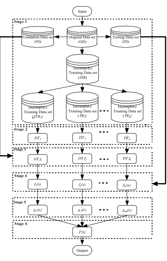
Our proposed method uses DTs as its component classifier. The main objective is to combine predictions of this classifier. A motivation for ensemble is that a combination of outputs of many weak MDTs produces a powerful ensemble MDTs with higher accuracy than a single MDT obtained from the same sample. The proposed method makes use of all data available and utilises a systematic pattern of classification results based on two methods for handling incomplete training and test data. The new generalized algorithm is summarised in Fig. 2, with the overall six-stage scheme of the technique shown in Fig. 3 and described in more detail in the following sections.
4.3.1. Partitioning original dataset
Due to the shortage in some data analysis problems, such approaches, such as bagging [2] have been used for creating samples varying the data subsets selected. The bagging algorithm is very efficient in constructing a reasonable size of training set due to the feature of its random sampling with replacement. Therefore such a strategy (which we also use in this study) is a useful data preparation method for ML.
4.3.2. Creating diverse decision tree classifier
Diversity in ensemble of learnt models constitute one of the main current directions in ML and data mining. It has been shown theoretically and experimentally that in order for an ensemble to be effective, it should consist of high-accuracy base classifiers that should have high diversity in their predictions. One technique, which proved to be effective for constructing an ensemble of accurate and diverse base classifiers, is to use different training data, or so-called ensemble training data selection. Many ensemble
Input Output DTn DT2 DT fn DT f2 DT f1 fm(x) fs(x) f1(x) gm(x) g2(x) g1(x) F(x) DT1
Testing Data set
(TD)
Validation Data set
(VD)
Original Data set
(OD)
Incomplet e Training Data set
(TRn)
Incomplet e Training Data set
(TR2)
Incomplet e Training Data set
(ITR1)
Incompelt e Training Data set
(ITR) . Stag e 1 Stage 4 Stage 5 Stage 6 Stage 3 St age 2
training data selection strategies generate multiple classifiers by applying a single learning algorithm, to different versions of a given dataset, Two different methods for manipulating the dataset are normally used: random sampling with replacement (also called bootstrap sampling) in bagging and re-weighting of the misclassified training instances in boosting. In our study, bagging is selected.
4.3.3. Decision tree learning
A brief description of DTs has already been given in Section 3 of the paper. Many variants of DT algorithms have concentrated on DTs in which each node checks the value of a single attribute. This class of DTs may be called axis – parallel because the tests at each node are equivalent to hyper-planes that are parallel to axes in the attribute space, i.e., they correspond to partitioning the parameter space with a set of hyper-planes that are parallel to all the features axes except for the one being tested and are orthogonal to that one.
In axis – parallel decision methods, a tree is constructed in which at each node a single parameter is compared to some constant. If the feature value is greater than the threshold, the right branch of the tree is taken; if the value is smaller, the left branch is followed.
There are DTs that test a linear combination of the attributes at each internal node. They allow the hyper-planes at each node of the tree to have any orientation in parameter space [42,43]. Mathematically, this means that at each node a linear combination of some or all the parameters is computed (using a set of feature weights specific to that node) and the sum is compared with a constant. The subsequent branching until a leaf node is reached is just that used for axis parallel trees.
Since these tests are equivalent to an oblique orientation to the axes, we call this class of trees oblique DTs. Note that oblique DTs produce polygonal (polyhedral) partitioning of the attribute space. Oblique DTs are also considerably more difficult to construct than axis parallel trees because there are so many more possible planes to consider at each node. As a result, the training process is slower. This is one the major reasons why axis-parallel DTs are considered in our study.
4.3.4. Selecting appropriate ensemble members
After training, each individual DT grown by using different MDTs has generated its own result. However, if there is a great number of individual members (i.e., MDTs, hence, in part, DTs), we need to select a subset of representatives in order to improve ensemble efficiency. Furthermore, it does have to follow the rule ‘the more the better’ rule as mentioned by some researchers. In this study, a de-correlation maximization method [24,34] is used to select the appropriate number of DTs ensemble members. The idea is that the correlations between the selected MDTs, thus, DT classifiers, should be as small as possible. The de-correlation matrix can be summarized in the following steps:
1. Compute the variance-covariance matrix and the correlation matrix
2. For theithDT classifier (i=1, 2,. . .,p), calculate the plural-correlation coefficienti
3. For a pre-specified thresholdθ, ifi < θ, then theithclassifier should be deleted from thepclassifiers. Conversely, ifi > θ, then theithclassifier should be retained.
4. For the retained classifiers, perform Eqs (1–3) procedures iteratively until satisfactory results are obtained.
4.3.5. Performance measure evaluation
In the previous phase the DT classifier outputs are used as performance evaluation measures (in terms of misclassification error rates). It has often been argued that selecting and evaluating a classification model based solely on its error rates is inappropriate. The argument is based on the issue of using
both the false positive (rejecting a null hypothesis when it is actually true) and false negative (failing to reject a null hypothesis when it is in fact false) errors as performance measures whenever classification models are used and compared. Furthermore, in the business world, decisions (of the classification type) involve costs and expected profits. The classifier is then expected to help making the decisions that will maximise profits. For example, predicting development effort of software systems involves two types of errors: 1) predicting software effort as likely to be high when in fact it is low, and 2) predicting software effort development as likely to be low when in fact it is high. Now, mere misclassification rate is simply not good enough to predict software effort. To overcome this problem and further make allowances for the inequality of mislabelled classes, variable misclassification costs are incorporated in our attribute selection criterion via prior specification for all our experiments. This also solves the imbalanced data problem. Details about how misclassification costs are used for both splitting and pruning rules are presented in [4].
4.3.6. Integrating multiple classifiers into ensemble output
Depending upon the work in the previous stages, a set of appropriate number of ensemble members can be identified. The subsequent task is to combine these selected members into an aggregated classifier in an appropriate ensemble strategy. Common strategies to combine these single DT results and then produce the final output are simple averaging; weighted averaging, ranking and majority voting. For more information on these strategies, the reader is referred to [14], which are otherwise briefly discussed below.
Simple averaging is one of the most frequently used combination methods. After training the members
of the ensemble, the final output can be obtained by averaging the sum of each output of the ensemble members. Some experiments have shown that simple averaging is an effective approach [3].
Weighted averaging is where the final ensemble result is calculated based on individual ensemble
members’ performances and a weight attached to each individual member’s output. The gross weight is 1 and each member of an ensemble is entitled to a portion of this gross weight according to their performance or diversity.
Ranking is where members of the ensemble are called low level classifiers and they produce not only
a single result but a list of choices ranked according to their likelihood. Then the high level classifier chooses from these set of classes using additional information that is not usually available to or well represented in a single low level classifier.
Majority voting is the most popular combination method for classification problems because of its
easy implementation. Members of trees voting decide the value of each output dimension. It takes over half the ensemble to agree a result for it to be accepted as the final output of the ensemble (regardless of the diversity and accuracy of each tree generalization). Majority voting ignores the fact that some trees that lie in a minority sometimes do produce correct results. However, this is the combination strategy approach we follow in our study.
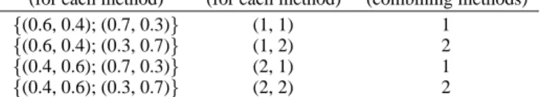
The following example demonstrates the mechanics of the proposed procedure as presented in Table 3. Suppose that there are two methods used to handle incomplete data when growing decision trees, resulting in two trees. Also, there are only two classes in the data: 1 and 2. Using the predicted probabilities, there are four possible classification patterns from the training data such as (1, 1), (1, 2), (2, 1) (2, 2). The first element in each pair denotes the class predictions by DT1and the second by DT2. If the instance has predictions (1, 1) for both methods, it is simply assigned class 1 anyway. However, if the instance has predictions (1, 2) it is assigned to the class with the higher overall probability which in this case happens to be 2, and so on.
Table 3 An example pattern table
Predicted probabilities Predicted class Predicted class (for each method) (for each method) (combining methods) {(0.6, 0.4); (0.7, 0.3)} (1, 1) 1
{(0.6, 0.4); (0.3, 0.7)} (1, 2) 2 {(0.4, 0.6); (0.7, 0.3)} (2, 1) 1 {(0.4, 0.6); (0.3, 0.7)} (2, 2) 2
5. Related work
Several researchers have examined various techniques to solve the problem of incomplete data in SE. One popular approach includes discarding instances with missing values and restricting the attention to the completely observed instances, which is also known as listwise deletion (LD). This is the default in commonly used statistical packages such s SPLUS [73]. Another common way uses imputation (estimation) approaches that fill in a missing value with an efficient single replacement value, such as the mean, mode, hot deck, and approaches that take advantage of multivariate regression and k-NN models. Another technique for treating incomplete data is to model the distribution of incomplete data and estimate the missing values based on certain parameters. Specific results are discussed below.
Lakshminarayan et al. [35] performed a simulation study comparing two ML methods for missing data imputation using an industrial process maintenance dataset of 82 variables and 4383 instances. Their results show that for the single imputation task, the SL algorithm C4.5, which utilizes the fractioning of cases (FC) strategy, performed better than Autoclass [9], a strategy based on unsupervised Bayesian probability. For the MI task, both methods performed comparably.
MI was used by El-Emam and Birk [16] to handle missing values in their empirical study that evaluated the predictive validity of the capability measures of the ISO/IEC 15504 software development processes (i.e., develop software design, implement software design, and integrate and test). The study was conducted on 56 projects. For large organizations their results provided evidence of predictive validity which was found to be strong while for small organizations the evidence was rather weak.
The pioneering work by Strike et al. [62] performed a comprehensive simulation study to evaluate three MDTs in the context of software cost modelling. These techniques are LD, mean or mode single imputation (MMSI) and eight different types of hot deck single imputation (HDSI). A dataset composed of 206 software projects and 26 different companies was used. Their results show LD as not only having a severe impact on regression estimates but yielding a small bias as well. However, the precision of LD worsens with increases in missing data proportions. Their results further show that better performance would be obtained from applying imputation techniques.
Another comparative study of LD, mean or mode single imputation (MMSI), similar response pattern imputation (SRPI) and full information maximum likelihood (FIML) in the context of software cost estimation was carried out by Myvreit et al. [44]. The simulation study was carried out using 176 projects. Their results show FIML performing well for data that is not MCAR. LD, MMSI and SRPI are shown to yield biased results for data other than MCAR.
The performance of k−NNSI and sample mean imputation (SMI) was analyzed by Cartwright et al. [7] using two industrial datasets; one dataset from a bank (21 completed projects) and the other from a multinational company (17 projects). Their results show both methods yielding good results withkNNSI providing a more robust and sensitive method for missing value estimation than SMI.
Song and Shepperd [63] evaluatedkNNSI and class mean imputation (CMI) for different patterns and mechanisms of missing data The dataset used for the study is the ISBSG database with 363 complete
instances. Their results showkNNSI slightly outperforming CMI with the missing data mechanisms having no impact on either of the two imputation methods.
Thek−NNSI method was evaluated using a likert dataset with 56 cases in the SE context by J ¨onsson and Wohlin [25]. Their results not only showed that imputing missing likert data using thek-nearest neighbour method was feasible but also showed that the outcome of the imputation depends on the number of complete cases more than the proportion of missing data. Their results further showed the importance of choosing an appropriatekvalue when using such a technique.
The use of multinomial logistic regression imputation (MLRI) for handling missing categorical values on a datataset on 166 projects of the ISBSG multi-organizational software database was proposed by Sentas et al. [59]. Their proposed procedure was compared with LD, MMSI, Expectation-Maximization single imputation (EMSI) and regression-based single imputation (RBSI). Their results showed LD and MMSI as efficient when the percentage of missing values is small while RBSI and MLRI were shown to outperform LD and MMSI as the amount of missing values increased. Overall, MLRI gave the best results, especially for MCAR and IM data. For MAR data, MLRI compared favourably with RBSI.
Twala et al. [71] evaluates the impact of seven MDTs {LD, EMSI, 5-NNSI, MMSI, MI, FC and surrogate variable splitting (SVS)}on eight industrial datasets by artificially simulating three different proportions, two patterns and three mechanisms of missing data. Their results show MI achieving the highest accuracy rates with other notably good performances by methods such as FC, EMSI and
kNNSI. The worst performance was by LD. Their results further show MCAR data as easier to deal with compared with IM data. Twala [68] further found missing values as more damaging when they are in the test sample than in the training sample. MIA was shown to be the most effective method when dealing with incomplete data using DTs especially for IM data [69]. The superior performance of MI and the severe impact of IM data on predictive accuracy is also observed in [67].
Despite the scarcity and small sizes of software data and the fact that the LD procedure involves an efficiency cost due to the elimination of a large amount of valuable data, most SE researchers have continued to use it due to its simplicity and ease of use. However, by sacrificing a large amount of data, the sample size is severely reduced. There are other problems caused by using the LD technique. For example, elimination of instances with missing information decreases the error degrees of freedom in statistical tests such as the studenttdistribution. This decrease leads to reduced statistical power (i.e. the ability of a statistical test to discover a relationship in a dataset) and larger standard errors. In extreme cases this may mean that there is insufficient data to draw any useful conclusions from the study. Other researchers have shown that randomly deleting 10% of the data from each attribute in a matrix of five attributes can easily result in eliminating 59% of instances from analysis [27,33].
As for the SI techniques, the results are not so clear, especially for small amounts of missing data. However, the performance of each technique differs with increases in the amount of missing data. Several shortcomings of single imputation have been documented by Little and Rubin [36], Schafer and Graham [57] and others. The obvious limitation is that it cannot reflect sampling variability under one model for nonresponse or uncertainty about the correct model for nonresponse, i.e. it does not account for the uncertainty about the prediction of the imputed values. The lack of sampling variability could distort estimates, standard errors, and hypothesis tests, leading to statistically invalid inferences [36].
MI, which overcomes limitations of single imputation methods by creating an inference that validly reflects uncertainty of prediction of the missing data, seem not to have been widely adopted by researchers. This is despite the fact that MI has been shown to be flexible, and software for creating MIs is available and some downloadable free of charge.1
Table 4
Datasets used for the experiments* Dataset Instances Attributes
Numerical Categorical Number of classes (distribution) Kemerer 18 4 2 1 (24.1%); 2 (75.9%) Bank 18 2 7 1 (84.3%); 2 (15.7%) Test equipment 16 17 4 1 (43.0%); 2 (57.0%) DSI 26 5 0 1 (49.9%); 2 (50.1%) Moser 32 1 1 1 (42.2%); 2 (57.8%) Desharnais 77 3 6 1 (15.7%); 2 (84.3%) Finnish 95 1 5 1 (57.0%); 2 (43.0%) ISBSG version 7 166 2 7 1 (35.6%); 2 (64.4%) CCCS 282 8 0 1 (48.2%); 2 (51.8%) Company X 10434 4 18 1 (33.0%); 2 (29.2%); 3 (37.8%) *after the removal of instances with missing attribute values.
6. Experimental set-up 6.1. Introduction
Incomplete data has been shown to have a negative impact in reducing ML performance in terms of predictive accuracy while the use of an ensemble of classifiers strategy has been shown to improve predictive accuracy by aggregating the predictions of many classifiers. In this regard, two sets of experiments based on ten industrial datasets (see Table 4) are carried out. Of these datasets, a couple were obtained from the Promise SE repository [54] and others, like ISBSG [23], from researchers at various software companies. Nearly all the datasets used for the experiments have missing values. The objective is to have control over of how different missing data patterns and mechanisms are simulated on a complete dataset. Thus, all instances with missing values were initially removed using LD (which assumes missing values are MCAR) before starting the experiment.
The response or class attribute (software effort) is continuous for all the datasets. However, in this paper we are dealing with a classification-type of problem that predicts values of a categorical dependent attribute from one or more continuous or categorical attribute values. Therefore, software effort was made discrete into a set of three disjoint categories for all datasets. The rule induction technique [15, 49] was utilized for this task. The cut-points were determined in a way that was not blinded to the class attribute, hence, achieving unbiased effect estimates. Monte Carlo simulations which take into account both multiplicities and uncertainty in the choice of cut-points were also utilized for this task [22]. For example, for the Company X dataset, the three categories used were: (low effort, when EFFORT<= 5000; medium effort, when 5000<EFFORT<=10000; high effort, when EFFORT>10000).
5-fold cross validation was used for tree induction for the experiments. For each fold, four of the parts of the instances in each category were placed in the training set, and the remaining one was placed in the corresponding test as shown in Table 5.
Since the distribution of missing values among attributes (pattern) and the missing data mechanism were two of the most important dimensions of this study, three suites of data were created corresponding to MCAR, MAR and IM. In order to simulate missing values on attributes, the original datasets are run using a random generator (for MCAR) and a quantile attribute-pair approach (for both MAR and IM, respectively). Both of these procedures have the same percentage of missing values as their parameters. These two approaches were also run to get datasets with four levels of proportion of missingnessp, i.e.,
Table 5
Partitioning of dataset to training and test sets
Training set Test set
Fold 1 Part II+Part III+Part IV+Part V Part I Fold 2 Part I+Part III+Part IV+Part V Part II Fold 3 Part I+Part II+Part IV+Part V Part III Fold 4 Part I+Part II+Part III+Part V Part IV Fold 5 Part I+Part II+Part III+Part IV Part V
0%, 15%, 30% and 50% missing values. The experiment consists of havingp% of data missing from both the training and test sets.
6.2. Modelling of missing data mechanisms
The missing data mechanisms were constructed by generating a missing value template (1=present, 0=missing) for each attribute and multiplying that attribute by a missing value template vector. Our assumption is that the instances are independent selections.
For each dataset, two suites were created. First, missing values were simulated on only half of the attributes. Second, missing values were introduced on all the attribute variables. For both suites, the missingness was evenly distributed across the attributes. This was the case for the three missing data mechanisms, which from now on shall be called MCARhalf, MARhalf, IMhalf (for the first suite) and MCARunifo, MARunifo, IMunifo(for the second suite). These procedures are described below.
For MCAR, each vector in the template (values of 1’s for non-missing and 0’s for missing) was generated using a random number generator utilising the Bernoulli distribution. The missing value template is then multiplied by the attribute of interest, thereby causing missing values to appear as zeros in the modified data.
Simulating MAR values was more challenging. The idea is to condition the generation of missing values based upon the distribution of the observed values. Attributes of a dataset are separated into pairs, say, (Ax, AY), where AY is the attribute into which missing values are introduced and AX is the attribute on the distribution of which the missing values of AY is conditioned, i.e., P(AY =miss| Ax=observed). The pairing of attributes was based on how highly correlated to one another they were. So, highly correlated attributes was paired against each other. Since we want to keep the percentage of missing values at the same level overall, we had to alter the percentage of missing values of the individual attributes. Thus, in the case of k% of missing values over the whole dataset, 2k% of missing values were simulated on AY. For example, having 10% of missing values on two attributes is equivalent to having 5% of missing values on each attribute. Thus, for each of the Ax attributes its 2kquantile was estimated. Then all the instances were examined and whenever theAX attribute has a value lower than the 2kquantile a missing value on AY is imputed with probability 0, and 1 otherwise. More formally, P(AY= miss|Ax <2k)=0 or P(AY =miss|Ax >2k)=1. This technique generates a missing value template which is then multiplied withAY. Once again, the attribute chosen to have missing values was the one highly correlated with the class variable. Here, the same levels of missing values are kept. For multi-attributes, different pairs of attributes were used to generate the missingness. Each attribute is paired with the one it is highly correlated to. For example, to generate missingness in half of the attributes for a dataset with, say, 12 attributes (i.e. A1,. . ., A12), the pairs (A1, A2), (A3 ,A4) and (A5, A6) could be utilised. We assume that A1will be highly correlated with A2; A3 highly correlated with A4, and so on. For the (A1, A2) pairing, A1 is used to generate a missing value template of zeros and
ones utilizing the quantile approach. The template is then used to “knock off” values (i.e., generating missingness) in A2, and vice versa.
In contrast to the MAR situation outlined above where data missingness is explainable by other measured variables in a study, IM data arise due to the data missingness mechanism being explainable, and only explainable by the very variable(s) on which the data are missing. For conditions with data IM, a procedure identical to MAR was implemented. However, for the former, the missing values template was created using the same attribute variable for which values are deleted in different proportions.
For consistency, missing values were generated on the same attributes for each of the three missing data mechanisms. This was done for each dataset. For split selection, the impurity approach was used. For pruning, we use 5-fold cross validation cost complexity pruning and 1 Standard Error (1-SE) rule in CART to determine the optimal value for the complexity parameter [4]. The same splitting and pruning rules when growing the tree were carried out for each of the ten industrial datasets.
6.3. Performance evaluation
A classifier was built on the training data and the predicted accuracy is measured by the smoothed classification error rate of the tree, and was estimated on the test data. Instead of summing terms that are either zero or one as in the error-count estimator, the smoothed misclassification error rate uses a continuum of values between zero and one in the terms that are summed. The resulting estimator has a smaller variance than the error-count estimate. Also, the smoothed error rate can be very helpful when there is a tie between two competing classes. This is the main reason why it was considered for our experiments.
It was reasoned that the condition with no missing data should be used as a baseline and what should be analysed is not the error rate itself but the increase or excess error induced by the combination of conditions under consideration. Therefore, for each combination of method for handling incomplete data, the number of attributes with missing values, proportion of missing values, and the error rate for all data present was subtracted from each of the three different proportions of missingness. This would be the justification for the use of differences in error rates analysed in some of the experimental results. All statistical tests were conducted using the MINITAB statistical software program [39]. Analyses of variance, using the generalized linear model procedure [32] were used to examine the main effects and their respective interactions. This was done using a 4-way repeated measures design (where each effect was tested against its interaction with datasets). The fixed effect factors were the: missing data techniques; number of attributes with missing values (missing data patterns); missing data proportions; and missing data mechanisms. A 1% level of significance was used because of the many number of effects. Results were averaged across five folds of the cross-validation process before carrying out the statistical analysis. The averaging was done as a reduction in error variance benefit.
Numerous measures are used for performance evaluation in ML. In predictive knowledge discovery, the most frequently used measure is predictive accuracy. To measure the performance of MDTs and the ensemble MDTs, the training set/test set methodology is employed. Unfortunately, an operational definition of accurate prediction is hard to come by. However, predictive accuracy is mostly operationally defined as the prediction with the minimum costs (the proportion of misclassified instances). The need for minimizing costs, rather than the proportion of misclassified instances, arises when some predictions that fail are more catastrophic than others, or when some predictions that fail occur more frequently than others. Minimizing costs, however, does correspond to minimizing the proportion of misclassified instances when priors are taken to be proportional to the class sizes and when misclassification costs are taken to be equal for every class. This is the approach we follow in the paper.
Khoshgoftaar and Seliya [28] and Khoshgoftaar et al. [31] argue that in the context of the software development, selecting and evaluating a classification model (like a DT) based solely on its error rates is inappropriate. Their argument is based on the issue of using both the false positive (rejecting a null hypothesis when it is actually true) and false negative (failing to reject a null hypothesis when it is in fact false) errors as performance measures whenever classification models are used and compared. Furthermore, in the business world, decisions (of the classification type) involve costs and expected profits. The classifier is then expected to help making the decisions that will maximise profits. CART is able to handle this problem in terms of taking into account misclassification costs when constructing the DT.
6.4. Programs and codes for methods
No software or code was used for LD. Instead, all instances with missing values on that particular attribute were manually excluded or dropped, and the analysis was applied only to the complete instances. S-PLUS code was also developed for the MMSI approach. The code was developed in such a way that it replaced the missing data for a given attribute by the mean (for a numerical or quantitative attribute) or mode (for a nominal or qualitative attribute) of all known values of that attribute.
An index structure M-tree [11] was used as a representative of the k-NN approach for handling missing attribute values in both the training and test samples. This technique can organize and search datasets based on a generic metric space. In addition, it can drastically reduce the number of distance computations in similarity queries. The missing values were estimated using 1, 3, 5, 11, 15, 21 nearest neighbours. However, only results with5-nearest neighbour will be showed in this work.
From the MIA method, an unknown (missing) value is considered an additional attribute value. Hence, the number of values is increased by one of each attribute that depicts and unknown value in the training or test set. S-PLUS code for this method was developed.
There are many implementations of MI. Schafer’s [55] set of algorithms (headed by the NORM program) that use iterative Bayesian simulation to generate imputations was an excellent option. NORM was used for datasets with only continuous attributes. A program called MIX written was used for mixed categorical and continuous data. For strictly categorical data, CAT was used. All three programs are available as S-PLUS routines.
For the SVS method, the RPART routine, which implements within S-PLUS many of the ideas found in the CART book and programs of Breiman et al. [4] was used for both training and testing DTs.
The DTSI method uses a DT for estimating the missing values of an attribute and then uses the data with filled values to construct a DT for estimating or filling in the missing values of other attributes. An S-PLUS code to estimate missing attribute values using a DT for both incomplete training and test data was developed.
The DT learner C4.5 was used as a representative of the FC or probabilistic technique for handling missing attribute values. This technique is probabilistic in the sense that it constructs a model of the missing values, which depends only on the prior distribution of the attribute values for each attribute tested in a node of the tree. The main idea behind the technique is to assign probability distributions at each node of the tree. These probabilities are estimated based on the observed frequencies of the attribute values among the training instances at that particular node.
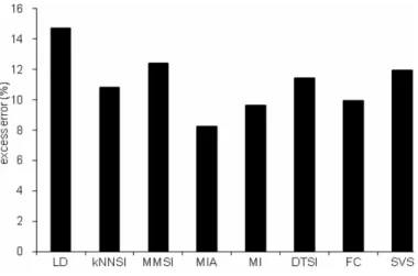
Fig. 4. Overall means for current methods.
6.5. Experiments 6.5.1. Experiment I
In order to empirically evaluate the performance of the eight MDTS on predictive accuracy, an experiment on ten industrial datasets is (given in Table 2) is used. This experiment is carried out in order to rank individual MDTs and also assess the impact of missing data (at various levels) on software predictive accuracy.
6.5.1.1. Experimental results I
Experimental results on the effects of current methods for handling both incomplete training and test data on predictive accuracy using DTs are described. The behaviour of these methods is explored for different patterns, levels of missing values, and for the mechanism of missing data. The error rates of each method of dealing with the introduced missing values are averaged over the ten datasets. Also, all the error rates increases over the complete data case are formed by taking differences. From these experiments the following results are observed.
Main effects
All the main effects were found to be significant at the 1% level of significance (F=61.95, df=7 for MDTs; F=19.36, df=1 for number of attributes with missing values; F=201.54, df=2 for missing data proportions, F=112.80, df=2 for missing data mechanism;p <0.01 for each).
From Fig. 4, MIA is the overall best technique for handling incomplete data with an excess error rate of 8.2%, closely followed by MI, FC andk-NNSI, with excess error rates of 9.6%, 9.9% and 10.8, respectively. The worst technique is LD, which exhibits an error rate of 14.7%.
Tukey’s multiple comparison tests showed no significant differences between DTSI and MMSI (on the one hand) and MIA and MI (on the other hand). However, significant differences are observed between MI and the other single imputation strategies like DTSI,k-NNSI and MMSI. The two SL strategies (FC and SVS) were found to be significantly different from each other. 5-NNSI and FC were found to be not significantly different from each other. The significance level for all the comparison tests is 0.01. All interaction effects we found to be insignificant at the 1% level of significance. Hence, they are not discussed in the paper.
Fig. 5. Overall means for current techiniques and ensembles.
6.5.2. Experiment II
The main objective of this experiment is to compare the performance of the new ensemble method with current approaches to deal with the problem of incomplete data, especially the top three MDTs that exhibited higher accuracy rates in the previous experiment. These include MI, MIA and FC. Also, we thought it would be interesting to test the effectiveness of the proposed approach with a statistical imputation technique (MI), a new approach (MIA) and a SL technique (FC). From the combination of three MDTs, three different ensembles methods are also proposed as given below:
i. MIAMI, a component of MIA and MI ii. MIAFC, a component of MIA and FC; and iii. MIFC, a component of MI and FC
The above three ensemble methods are also compared with each of the three MDTs, individually.
6.5.2.1. Experimental results II Main effects
All the main effects were found to be significant at the 1% level of significance (F=84.5, df=5 for existing and ensemble missing data methods; F=26.3, df =1 for number of attributes with missing values; F=73.8 df=2 for missing data proportions, F=36.4, df=2 for missing data mechanism;p < 0.01 for each).
Figure 5 shows the average results of 180 experiments (3 MDTs plus 3 ensemble methods x 2 missing data patterns x 3 missing data proportions x 3 missing data mechanisms) which summarizes imputation accuracy of each method. The accuracies of each method are averaged over the ten datasets. Figure 5 further shows that the MIAMI ensemble has on average the best accuracy throughout the entire spectrum missing data proportions, patterns, and mechanisms. Tukey’s multiple comparison tests showed significant differences between MIAMI and the other individual MDTs at the 1% level.
Interaction effects
Only two two-way interactions effects were found to be statistically significant at the 1% level. These are: the interaction between current and new MDTs, ensemble methods and missing data pattern (F= 8.45, df=12;p <0.01), and the interaction between current and new MDTs and ensemble methods and missing data mechanisms (F=13.8, df=18;p <0.01).
Fig. 6. Interaction between methods and missing data patterns.
Fig. 7. Interaction between missing data techiniques and missing data mechanisms.
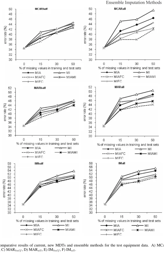
The interaction effect between the ensemble and MDTs and the missing data patterns is shown in Fig. 6. This figure shows all the methods performing better when the missing values are in all the attributes compared with when they are only in half of the attributes.
In addition, the impact of missing data patterns appears to differ by the type of missing data method. For example, MI exhibits one of the biggest increases in error rates (as the number of attributes with missing values increases) compared with only a very small increase achieved by MIA. Figure 7 shows all techniques achieving bigger error rates when dealing with IM data compared with either MCAR or MAR data. From the three ensemble methods, the most affected is MIAFC, especially for IM data. In addition, some techniques appear to be severely impacted by the different missing mechanisms than others.
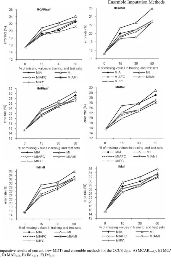
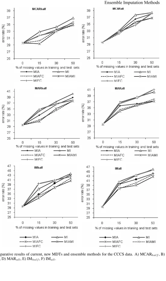
6.5.3. Results for individual Datasets: Current and New MDTs Vs. Ensemble Methods
The results that illustrate specific deviations from the overall results of the effectiveness of the new ensemble methods against the current and new MDTs for constructing and classifying incomplete vectors on different database characteristics, especially on datasets where the new method yielded superior performance compared with MIA, MI and FC, are given below.