A Fast Explicit FETD Method Based on Compressed Sensing
Qi Qi1, 2, Mingsheng Chen2, *, Zhixiang Huang1, Xinyuan Cao2 and Xianliang Wu1
Abstract—Linear equations must be solved at each time step as the explicit finite element time-domain (FETD) method is used to solve time dependent Maxwell curl equations, which leads to a huge amount of computational cost in a long period time simulation. A new scheme to accelerate the iteration solution for matrix equation is proposed based on compressed sensing (CS), in which a low rank measurement matrix is established by randomly extracting rows from mass matrix. Meanwhile, to reduce the number of measurements required, a sparse transform is constructed with the help of prior knowledge offered by the solution results of previous time steps. Numerical results of homogeneous cavity and inhomogeneous cavity are discussed to validate the effectiveness and accuracy of the proposed approach.
1. INTRODUCTION
Finite element time-domain method (FETD) is an efficient tool for solving electromagnetic scattering problems, since it combines the advantages of time-domain techniques with the versatile spatial discretization options of the finite element method (FEM) [1]. It is easy to use FETD to handle multi-scale geometry and acquire information over a wide frequency band. Sorts of FETD methods have been proposed in recent years, an explicit method that directly solving Maxwell curl equations utilizes the electric fieldEand magnetic flux intensityBas simultaneous state variables has been mentioned in [2, 3]. This mixed method can also be considered as a generalization of the finite-difference time-domain (FDTD) method for unstructured grids. Due to its potential effect to simulate free space conveniently by introducing perfectly matched layer [4] and conserve energy over long period time in conjugation with symplectic method [5], more attention has been devoted to it. However, the computation of interpolation coefficients of global variables E and B has to solve two matrix equations at each time step in this approach, which makes the calculation extremely expensive in a long period time simulation. Although reference [6] offered an improved scheme that only one matrix equation is required to be solved, this defect still limits its development and application.
Compressed sensing (CS) [7], as a current research focus in signal processing, has been introduced into biological engineering, communication engineering, image processing and electromagnetic field [8], etc. In CS theory, a signal can be captured at a rate significantly below the Nyquist rate if it has a sparse representation in a suitable transform domain, and then it can be exactly reconstructed using recovery algorithms [9]. By means of this theory, some useful schemes are developed to solve partial differential equations (PDEs) problems with the help of sparse approximations [10, 11].
Motivated by these early theoretical frameworks, a novel FETD method improved by CS (CS-FETD) is proposed to accelerate solution for the matrix equations of the mixed FETD method. The implementation of CS for this new scheme can be described by three steps: (1) establish a measurement matrix by randomly extracting some rows from mass matrix; (2) construct a new basis based on redundant dictionary that offered by the prior knowledge included in solutions of previous time steps;
Received 11 February 2017, Accepted 25 March 2017, Scheduled 3 April 2017
* Corresponding author: Mingsheng Chen ([email protected]).
1 Key Laboratory of Intelligent Computing and Signal Processing, Anhui University, Hefei 230039, China. 2 School of Electronic
The coupled first-order time dependent Maxwell curl equations in source free region are considered as
ε∂
∂tE = ∇ ×
μ−1B (1)
∂
∂tB = −∇ ×E. (2)
To achieve the FETD solution of Equations (1) and (2), the computational domain is assumed to be discretized by a FEM mesh with a triangle faces and d edges. The linear system of ordinary differential equations forT Ez problems are yielded by Galerkin FEM, in which Whitney 1-form vector
basis function is used to discretize electrical field intensity and Whitney 2-form vector basis function is used to discretize magnetic flux intensity, such as
[T]d×d∂
∂t{e}d×1 = [C]
T
a×d[K]a×a{b}a×1 (3)
∂
∂t{b}a×1 = −[C]a×d{e}d×1 (4)
where {e} and {b} are the interpolation coefficients of E and B, respectively, and [C] is the Curl operator. [T] is the 1-form mass matrix with the material property function is used to represent the dielectric properties, and [K] is the 2-form mass matrix with the material property functionμ−1 is used to represent the magnetic permeability. a and d define the dimension of mass matrix. Applying the leap frog method to (3) and (4) with a stable time step Δt, one can obtain
[T]d×d{e}nd×1 = [T]d×d{e} n−1
d×1 + Δt[C] T
a×d[K]a×a{b} n−1/2
a×1 (5)
{b}n+1/2a×1 = {b} n−1/2
a×1 −Δt[C]a×d{e}nd×1. (6)
2.2. Implementation of CS-FETD Method
The mathematical model of CS can be formulated as
[Φ]m×k{X}k×l= [Φ]m×k[Ψ]k×k{α}k×l= [S]m×l (7)
in which {α} is the sparse representation coefficients of original signal {X} with the sparse basis [Ψ], and [Φ] is the measurement matrix. m, k and l are the dimensions of these matrices, in general, k is much larger thanm. The approximation of{α} is computed by a L-minimization problem as
{ˆa}= min{a}k×lLs.t.[Φ]m×k[Ψ]k×k{ˆa}k×l= [S]m×l. (8) The process of CS discussed above is a regular application in signal processing and other fields. To implement CS in FETD method, some changes must be made in its procedure and they can be described as follows:
Step 1: At the beginning of the simulation,{e} is calculated by the traditional FETD method. Step 2: CS is implemented into FETD when the electromagnetic wave propagation covers the whole computation area. Based on (5) (the right side of (5) is denoted as{V}), an improved matrix equation
can be obtained as
Tf×d{e}d×1=
Vf×1 (9)
Figure 1. The variation of matrix equation (5) before and after the electromagnetic wave propagation covers the whole computation area.
be obtained as shown in Fig. 1, which is constituted of the column vectors of{e}obtained from previous time steps. In other words, the matrix is an existing redundant dictionary for{e}at the time step that is currently being calculated. Take [T] as the measurement matrix, Equation (9) at the i+ 1th time step can be transformed as
Tf×d[epre]d×i
ei×1=Vf×1 (10)
in which {e} represents the sparse projection of{e} in [epre]. Especially, sparse basis is required to be
updated over time. Fig. 1 shows the performance of Step 2.
Step 3: An appropriate recovery algorithm is applied to compute approximate value of{e}by
ˆ
e = min{e}Ls.t.T[epre] eˆ
=V (11)
{eˆ} = [epre]
ˆ
e. (12)
The complexity of CS-FETD is mainly decided by recovery algorithms after the application of CS. Taking orthogonal matching pursuit (OMP) technique as an example, the complexity is O(Sdf) [12], where S is the number of iteration steps. The complexity of traditional FETD by using the conjugate gradient (CG) algorithm to solve the matrix Equation (5) isO(P d2), whereP is similar toS. In general,
S P and f d, so that the proposed method is more efficient. Although the complexity of FETD can be decreased in virtue of the property that mass matrix is sparse and symmetric, CS-FETD also has the obvious advantage under the same conditions.
3. NUMERICAL RESULTS
To illustrate the effectiveness and accuracy by the proposed method, some resonant frequency problems of 2-D cavity with perfectly conducting walls in T Ez case are provided.
e
an accurate solution. Meanwhile, the resonant frequencies and computing time comparison are also described in Table 1. These comparison results demonstrate that CS-FETD has a high accuracy with relative error less than 0.1%, moreover requires only about half of the physical time of the conventional explicit formulation.
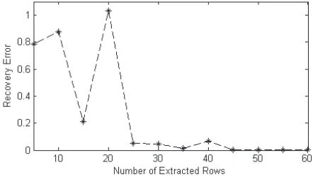
Figure 3. Relationship between recovery error and number of extracted rows at 2000th time step.
Figure 4. The interpolation coefficients of all edges at 1500th time step.
Table 1. Resonant frequencies of rectangle cavity.
f /d NO. steps Physical Time T E10 T E01, T E20 T E11
FETD 497/497 20000 3.914e3 s 7.500 15.000 16.667
CS-FETD 50/497 20000 2.146e3 s 7.500 15.000 16.658
3.2. Circular Cavity
Similar design principles are applied in the circular cavity case shown in Fig. 5. The dimension of mass matrix is 843×843 and the time step is set to be Δt= 0.9 ps.
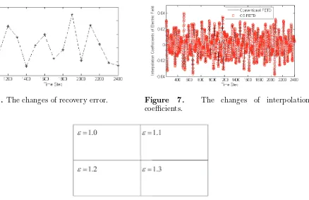
Figure 6 shows the recovery error changes from 1000th to 2400th time step with 70 rows extracted randomly from mass matrix. Fig. 7 depicts interpolation coefficients on certain an edge from 200th to 2400th time step with the same measurement times. Comparisons of computational results and physical time are shown in Table 2.
Table 2. Resonant frequencies of circular cavity.
f /d NO. steps Physical Time T E11 T E21 T E01
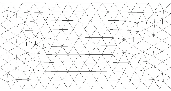
Figure 5. A circular cavity (r= 0.01 m) discretized with 843 edges and 546 triangle faces.
Figure 6. The changes of recovery error. Figure 7. The changes of interpolation coefficients.
Figure 8. A inhomogeneous cavity with four different dielectric properties areas.
3.3. Inhomogeneous Cavity
In this section, the rectangle cavity offered in the first example is divided into four areas with different dielectric properties. The inhomogeneous cavity depicted in Fig. 8 contains 540 edges and 344 triangles by FEM mesh. The time step is set to be Δt= 1.1 ps.
Figure 9. Relationship between recovery error and number of extracted rows at 3000th time step.
Figure 10. Recovery error changes.
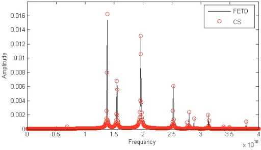
Figure 11. Comparison of resonant frequencies.
4. CONCLUSION
An improved scheme for accelerated FETD method based on CS theory is proposed, in which a low rank measurement matrix is extracted from mass matrix in FETD at each time step, and recovery algorithm is used instead of traditional iterative solution of matrix equations. Meanwhile, with the help of redundant dictionary formed by prior knowledge included in solutions of all previous time steps, the matrix dimension can be reduced drastically.
Numerical results have shown that the proposed method can reduce computing time without accuracy loss. Especially, it is worth mentioning that the proposed scheme can also be used to accelerate other time domain methods as there is a matrix equation to be solved.
ACKNOWLEDGMENT
REFERENCES
1. Lee, J. F., R. Lee, and A. C. Cangellairs, “Time-domain finite elements method,” IEEE Trans. Antennas Propagat., Vol. 52, No. 3, 2190–2195, 2004.
2. Wong, M., O. Picon, and V. F. Hanna, “A finite element method based on Whitney forms to solve Maxwell equations in the time domain,” IEEE Trans. Magn., Vol. 31, No. 3, 1618–1621, 1995. 3. Rieben, R. N., G. H. Rodrigue, and D. A. White, “A high order mixed vector finite element method
for solving the time dependent Maxwell equations on unstructured grids,”J. Computational Phys., Vol. 204, No. 2, 490–519, 2004.
4. Movahhedi, M., A. Abdolali, and H. Ceric, “Optimization of the perfectly matched layer for the finite-element time-domain method,”IEEE Microw. Wireless Compon. Lett., Vol. 17, No. 3, 10–12, 2007.
5. Rieben, R. N., G. H. Rodrigue, and D. A. White, “High-order symplectic integration methods for finite element solutions to time dependent Maxwell equations,” IEEE Trans. Antennas Propagat., Vol. 52, No. 8, 2190–2195, 2004.
6. He, B. and F. L. Teixeira, “Geometric finite element discretization of Maxwell equations in primal and dual spaces,”Phys. Lett. A, Vol. 349, No. 1–4, 1–14, 2006.
7. Baraniuk, R. G., “Compressive sensing,”IEEE Signal Proc. Mag., Vol. 24, No. 4, 118–121, 2007. 8. Chen, M. S. and F. L. Liu, “Compressive sensing for fast analysis of wide-angle monostatic
scattering problems,”IEEE Trans. Antennas Propagat., Vol. 10, No. 3, 1243–1246, 2011.
9. Tropp, J. A., J. N. Laska, and M. F. Duarte, “Beyond Nyquist efficient sampling of sparse band limited signals,” IEEE Trans. Inf. Theory, Vol. 56, No. 1, 520–544, 2010.
10. Mathelin, L. and K. A. Gallivan, “A compressed sensing approach for partial differential equations with random input data,” Commun. Comput. Phys., Vol. 12, No. 4, 919–954, 2012.
11. Caflisch, R. E., S. J. Osher, H. Schaeffer, and G. Tran, “PDEs with compressed solutions,”arXiv preprint arXiv:1311.5850v2, 2014.