Implementation of the Parallel Higher-Order FDTD
with Convolution PML
Yawen Liu1, 2, *, Pin Zhang2, and Yiwang Chen2
Abstract—In this paper, a parallel Higher-order FDTD (HO-FDTD) algorithm is described. Moreover, a novel implementation of convolution PML (CPML) is presented for the HO-FDTD method. A printed microstrip patch antenna is designed to analyze the feasibility of the parallel algorithm and the absorbing performance of the CPML. Moreover, the proposed algorithm is used to deal with the large-scale computational model of the vaulted tunnel. The simulation results show that the adopted parallel strategy is feasible, and the CPML performs well in the HO-FDTD scheme.
1. INTRODUCTION
The HO-FDTD [1–12] is an efficient numerical algorithm in the time-domain. Compared with the long established FDTD method [13], HO-FDTD method shows a highly-linear dispersion performance. So with the same accuracy, larger targets can be simulated with the HO-FDTD method. However, owing to the limitation of the computer memory, the calculation can be only implemented in a finite area. So, for the intensive computation and storage, there are some challenges for its practical implementation when dealing with the electrically large and complex electromagnetic structures. To overcome the computation power and storage requirement bottlenecks, this paper focuses on the parallel implementation of the HO-FDTD(2, 6). As the Message Passing Interface (MPI) [14] is becoming the new international standard for parallel programming, the MPI library is employed to exchange the electric and/or magnetic fields. For the sake of simplicity and compactness, a parallel HO-FDTD algorithm for the mode based on the one-dimension domain decomposition method is presented.
The CPML [15] is introduced to the HO-FDTD algorithm, and a planar microstrip-type structure in a 3-D case is analyzed with the parallel implementation and CPML. Furthermore, a computation model of the vaulted tunnel is established, and the impact of metallic door on the field cross-section distribution of the ultra-wideband electromagnetic pulse in the model is studied. Numerical results validate the feasibility of the parallel algorithm and the good absorbing effectiveness of the CPML.
2. PARALLEL HO-FDTD ALGORITHM
Just as the FDTD, HO-FDTD is also nearly inherently parallel in nature since only local information is needed for updating the fields at each time increment. Parallel HO-FDTD can be seen as a kind of algorithm that the whole computational domain is divided into several sub-domains, and each node only handles for the corresponding sub-domains calculation. Therefore, the requirement of computational storage and CPU time is reduced several times, which implies that the parallel HO-FDTD is faster than a serial counterpart almost by a factorn, wheren is the number of processors.
Received 22 August 2017, Accepted 21 September 2017, Scheduled 2 October 2017 * Corresponding author: Yawen Liu ([email protected]).
,
x
H Hy, Ex, Ey
1
nk
0
nk
x
E Ey Hx Hy
x
H Hy Ex Ey
Figure 1. Two adjacent sub-domains.
The domain decomposition method (DDM) is shown in Fig. 1, and this method uses an MPI function to send the Hx,y(:,:, nk1−1), Hx,y(:,:, nk1−2), Hx,y(:,:, nk1−3) and Ex,y(:,:, nk1−1), Ex,y(:
,:, nk1−2) from the processor N to N + 1, and to calculate the Ex,y(:,:, nk0), Ex,y(:,:, nk0 + 1),
Ex,y(:,:, nk0 + 2) and Hx,y(:,:, nk1 −1), Hx,y(:,:, nk1 −2) in processor N + 1. The MPI function is once again to send the Ex,y(:,:, nk0), Ex,y(:,:, nk0 + 1), Ex,y(:,:, nk0 + 2) and Hx,y(:,:, nk1 −1),
Hx,y(:,:, nk1−2) from the processorN + 1 toN.
3. APPLICATION OF CPML TO HO-FDTD METHOD
Following the implementation procedure described in [15], the formulation in the CPML layer is posed in the stretched coordinate space. In this work, a lossy medium is assumed for the sake of generality example. Thex-projection of Ampere’s law is thus specified as
jωεEx+σEx= 1
sy ∂ ∂yHz−
1
sz ∂
∂zHy, (1)
wheresi is the stretched-coordinate metric and defined as
si =κi+ σi
αi+jωε0
, i=x, y, z (2)
whereαi>0, σi >0, κi ≥1.
Defining thatsi =s−i 1, we can get:
s= 1
κi + σi
αi+jωεi, (3)
where σi =−σi, εi =ε0κi2 and αi=κi2αi+κiσi. Using Laplace transform theory, it can be shown that
si has the impulse response
si(t) = δ(t)
κi + σi εie
−αi
εitu(t) = δ(t)
whereδ(t) is the unit impulse function and u(t) the step function. Inserting Eq. (4) into Eq. (1), then transform Eq. (1) into time domain:
εrε0
∂Ex(t)
∂t +σEx(t)
= sy(t)∗ ∂
∂yHz(t)−s
z(t)∗∂z∂ Hy(t)
= 1
κy ∂
∂yHz(t)−
1
κz ∂ ∂zHy(t)
+
t
0
∂
∂yHz(t−τ)ζy(τ)dτ− t
0
∂
∂zHy(t−τ)ζz(τ)dτ (5)
The discrete impulse response for ζi(t) can be defined as
S0i(m) =
(m+1)Δt
mΔt
ζ(τ)dτ =− σi
ε0κ2i
(m+1)Δt
mΔt
e−
σi κiε0+αiε0
τ
dτ =aie−
σi κi+α
i mΔt
ε0 (6)
where
ai= σi
αi
e−
αi εiΔt−1
(7)
Then, inserting Eqs. (6) and (7) into Eq. (5), and according to the wavelet-Galerkin scheme based on Daubechies’ compactly supported wavelets, the MRTD equation forEx can be obtained as following
εrε0
Eϕx,n+1 i+12, j, k−E
ϕx,n i+12, j, k
Δt +σ
Eϕx,n+1 i+12, j, k+E
ϕx,n i+12, j, k 2
= 1
κyΔy
l
a(l)Hϕz, n+
1 2
i+12, j+l+12, k− 1
κzΔz
l
a(l)Hϕy, n+
1 2
i+12, j, k+l+12
+ 1 Δy
N−1
m=0
S0y(m)
l
a(l)Hϕz, n−m+
1 2
i+12, j+l+12, k− 1 Δz
N−1
m=0
S0z(m)
l
a(l)Hϕy, n−m+
1 2
i+12, j, k+l+ 12 (8)
whereEϕx,n
i+ 12, j, k,H
ϕy,n+12
i+12, j, k+12, and H
ϕz,n+12
i+12, j+12, k are the coefficients for the fields and the auxiliary variables expansions in terms of scaling functions which are equal to the corresponding fields. The indexes i,j,k, andn are the discrete space and time indices related to the space and time coordinates via x = iΔx, y = jΔy, z = kΔz, and t = nΔt, where Δx, Δy, Δz, and Δt represent the space and time discretization intervals inx-, y-,z- and t-directions. Defining that
ψnexy+1/2 =
N−1
m=0
Z0y(m)
l
a(l)Hϕz,n−m+
1 2
i+12, j+l+12, k (9)
ψnexz+1/2 =
N−1
m=0
S0z(m)
l
a(l)Hϕy, n−m+
1 2
i+ 12, j, k+l+12 (10) Then the following equations can be easily obtained:
ψenxy+1/2(i+ 1/2, j, k) = byψnexy−1/2(i+ 1/2, j, k) + ay Δy
l
a(l)Hϕz, n−m+
1 2
i+12, j+l+ 12, k (11)
ψenxz+1/2(i+ 1/2, j, k) = bzψnexz−1/2(i+ 1/2, j, k) + az Δz
l
a(l)Hϕy, n−m+
1 2
i+12, j, k+l+12 (12)
bi = e−
σi
κi+αi
Δt
and ai is given by Eq. (7). Then Eq. (8) can be rewritten as
Eϕx,n+1
i+12, j, k = CAmE
ϕx,n
i+12, j, k+CBm
1
κyΔy
l
a(l)Hϕz, n+
1 2
i+12, j+l+ 12, k
− 1
κzΔz
l
a(l)Hϕy, n+
1 2
i+12, j, k+l+12 +CBm
φϕx,n+
1 2
exy,i+ 12, j, k−φ
ϕx,n+ 12
exz,i+12, j, k
(14)
wherem= (i+12, j, k), and
CAm = 2εm−σmΔt
2εm+σmΔt, (15)
CBm = 2Δt
2εm+σmΔt (16)
From Eq. (14), we can see that the explicit time-marching schemes for the fields are obtained at the (n+ 1) time step. It is obvious that the CPML implementation is independent of the material medium, and the CPML implementation requires only two auxiliary variables per field component, which is less than that reported PML and APML [16, 17]. The coefficients a(l) are defined as [11]
a(l) = (−1)
l
2 (l+ 1/2)2
[(2L−1)!!]2
(2L−2−2l)!! (2L+ 2l)!! (17)
For simplicity, here we define L= 3, and the coefficients for 0≤l≤L−1 are shown in Table 1. The coefficients a(l) for l <0 are given by the symmetry relation a(−1−l) =−a(l).
Table 1. The coefficients a(l).
l a(l) 0 1.171875000
1 −0.065104167 2 0.004687500
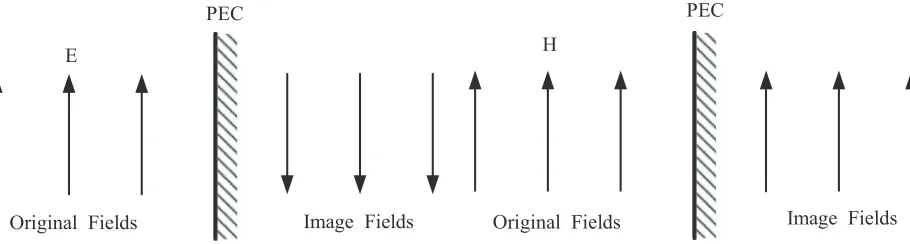
Moreover, we use perfectly electric conductor (PEC) walls to terminate the CPML regions. Since the HO-FDTD scheme does not allow localized boundary conditions, as shown in Fig. 2, the image technique is applied to the PEC boundaries.
PEC
E
Original Fields Image Fields
H
PEC
Original Fields Image Fields
Equations forEy and Ez are as follow:
Eϕy,n+1
i,j+ 12, k = CAmE
ϕy,n
i,j+12, k+CBm
1
κzΔz
l
a(l)Hϕx, n+
1 2
i,j+12, k+l+12
− 1
κxΔx
l
a(l)Hϕz, n+
1 2
i+ 12, j+l+12, k +CBm
φϕy,n+
1 2
eyz,i,j+12, k−φ
ϕy,n+ 12
eyx,i,j+ 12, k
(18)
Eϕz,n+1
i,j,k+12 = CAmE
ϕz,n
i,j,k+12 +CBm
1
κxΔx
l
a(l)Hϕy, n+
1 2
i+l+12, j, k+ 12
− 1
κyΔy
l
a(l)Hϕx, n+
1 2
i,j+l+12, k+12 +CBm
φϕz,n+
1 2
ezx,i,j,k+12 −φ
ϕz,n+12
ezy,i,j,k+12
(19)
The other set of equations for updating Hcan be obtained by duality.
4. NUMERICAL RESULTS
4.1. Computation Model of the Microstrip Patch Antenna
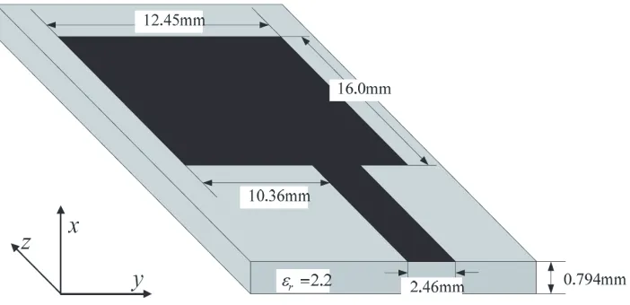
To check whether the parallel implementation is feasible or not, comparison between serial HO-FDTD and parallel HO-FDTD is executed to analyze a printed microstrip patch antenna, whose geometry is shown in Fig. 3.
Figure 3. Geometry and dimensions of the microstrip patch antenna.
A HO-FDTD mesh of 14×43×62 cells with Δx= 0.265 mm, Δy= 0.83 mm, Δz= 1.0 mm is used here. A ten-layer CPML is used to truncate both the HO-FDTD and lattices. The time discretization interval used for the HO-FDTD scheme is 0.3 ps scheme. We use the serial HO-FDTD and parallel HO-FDTD (4 PC nodes) to compute the case and then compare theS11 values. As shown in Fig. 4, we can conclude that parallel HO-FDTD gives the same result as serial HO-FDTD does, which validates the feasibility of the parallel FDTD and the availability of the CPML. However, the serial HO-FDTD will be helpless when huge grids are involved in the computation domain, and then only parallel HO-FDTD can work.
4.2. Computation of the Vaulted Tunnel with Metallic Door
Magnitude of S11
(dB)
2 4
-20 -15 -10 -5 0 5
4 6 8
Freq
10 12 1
quncy (GHz) Seria Paral
14 16 18
)
al HO-FDTD llel HO-FDTD
20 D
Figure 4. The magnitude of theS11 for the microstrip patch antenna.
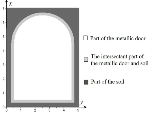
Figure 5. The computational model of the tunnel.
(a) (b)
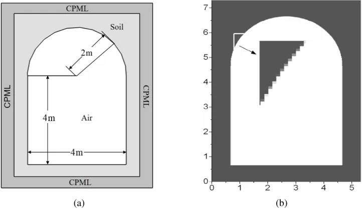
Figure 7. Profile of the computation model. (a) The cross-section of the tunnel. (b) The conformed vault of the tunnel.
place of z= 50.0 m. The source is placed near the CPML. For the purposes of this study, constitutive parameters for soil are assumed, giving σs = 0.004, εr = 9.0. The constitutive parameters for the wall and arris of the straight part can be defined as εeq = 9.0, σeq = σs/2 and εeq = (3ε0εr+ε0)/4,
σeq = 3σs/2.
The constitutive parameters for the wall and arris of the crooked part can be defined via the conformal technique [18]. The conformed vault of the tunnel is shown in Fig. 7(b).
In the waveguide system [13], the excitation source is usually introduced robustly according to propagation model such as TE10and TM11. Though in this case we cannot get the analytical model of the wave propagation, the way that the excitation sources induced in the waveguide system can still be employed here, which can be shown as follows
Etann+1(i, j, ks) =Etann (i, j, ks) +f(i, j, ks)g(t) (20) where the subscript ‘tan’ denotes the E-field distributed in a transverse cross section at z = ksΔz
of the tunnel structure in Fig. 5, f(i, j, ks) the function of the field distribution, and g(t) the time function determining the bandwidth of the sources. Here we setf(i, j, ks) to follow the model of TM11 propagation in waveguide with the size ofa×b= 4.0 m×6.0 m approximately, though the model does not satisfy the boundary condition of the tunnel, we can believe that after some length propagation, the model will be in a steady state which approaches TM11 propagation model of the tunnel itself.
TM11 propagation model is defined as
Ex =−jβ11
k2
c π aAcos
π ax sin π by
e−jβ11z
Ey =−jβ11
k2
c π bAsin
π ax cos π by
e−jβ11z Ez =Asinπaxsinπby e−jβ11z
Hx= jωε
k2
c π bAsin
π ax cos π by
e−jβ11z
Hy =−jωε
k2
c π aAcos
π ax sin π by
e−jβ11z Hz= 0
⎫ ⎪ ⎪ ⎪ ⎪ ⎪ ⎪ ⎪ ⎪ ⎪ ⎪ ⎪ ⎪ ⎪ ⎪ ⎪ ⎬ ⎪ ⎪ ⎪ ⎪ ⎪ ⎪ ⎪ ⎪ ⎪ ⎪ ⎪ ⎪ ⎪ ⎪ ⎪ ⎭ (21)
g(t) in Eq. (20) is defined as a differential Gaussian electric pulse that g(t) = E0(t −
t0) exp(4π(t−t0)2
τ2) with τ = 3.0 ns, E
an FDTD lattice with Δx = Δy = Δz = 0.0399 m, and ten-cell-thick PML layers terminate the grid. This results in a 170×129×2650 cell lattice, and time step is Δt= 57.589 ps. f(i, j, ks) is located at the
x-yplane withz= 0.2 m, and the sampling cross-section is located at thex-yplane withz= 49.9867 m and z= 51.0 m. The simulation have been performed for 10000 time steps.
To get a rather efficiently absorbing ability, the parameters of CPML can be shown as
⎧ ⎪ ⎪ ⎪ ⎨ ⎪ ⎪ ⎪ ⎩
σi =σmax
u−u0
dPML m
σmax=
m+ 1
150π√εrΔs, κi = 1 + (κmax−1)
|u−u0|
dPML
m (22)
where u = u0 is the boundary between computation domain and absorbing boundary and dP ML the thick of PML. In CPML, α can be set as a constant.
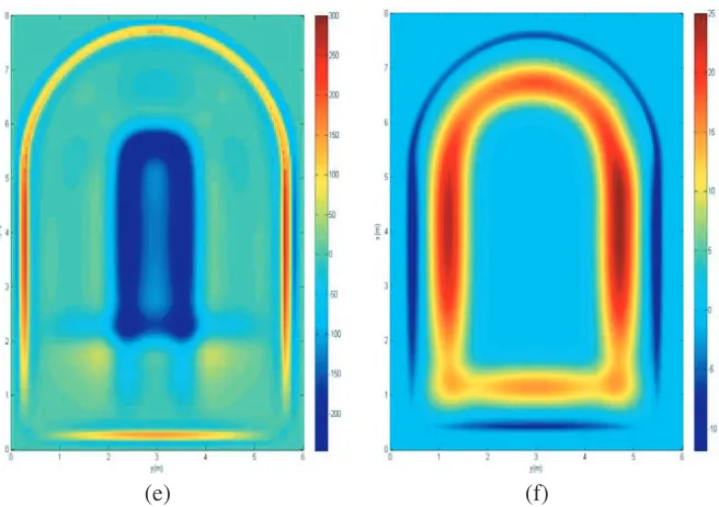
Figures 8(a) to 8(f) denote the cross-section distribution of the field ofEx, Ey and Ez excited by the TM11 propagation in the tunnel. “49.9867 m (265.0 ns)” means the filed value at the cross-section at the place of z= 49.9867 m when the time step reaches 265.0 ns, and the other is analogous.
(a) (b)
(e) (f)
Figure 8. The filed cross-section distribution. (a) Ex (V/m), 49.9867 m (265.0 ns). (b) Ex (V/m), 51.0 m (269.0 ns). (c)Ey (V/m), 49.9867 m (265.0 ns). (d)Ey (V/m), 51.0 m (269.0 ns). (e)Ez (V/m), 49.9867 m (265.0 ns). (f) Ez (V/m), 51.0 m (269.0 ns).
Observing the results, it is seen thatEx field basically distributes at the vault and the base of the tunnel, andEy field mainly distributes at the two sides, whereasEz field principally distributes around the tunnel. So it can be concluded how the filed gets into the space behind the metallic door: Ex field mainly circuitously propagates through the vault and the base, Ey filed through the two sides, andEz
field through circumambience of the metallic door. We can also summarize that along with the augment of the pulse propagation time, the energy of TM11 propagation model is centralized at the middle of the tunnel gradually.
5. CONCLUSION
In this paper, we present a parallel HO-FDTD approach. Details about the implementations of the domain decomposition, message passing between the neighboring processors are also provided, and the CPML is employed into the HO-FDTD method. It is shown that the CPML method requires only two auxiliary variables per discrete field component, which is less than that of the traditional PML and APML. Furthermore, two computation models of the microstrip patch antenna and the vaulted tunnel with metallic door are established Numerical results show that the parallel algorithm is feasible, and the CPML can provide a quite satisfactory absorbing boundary condition.
ACKNOWLEDGMENT
The authors would like to thank the reviewers for helpful remarks, and this work was supported by Natural Science Foundation of Jiangsu Province under Grant No. BK20150715.
REFERENCES
1. Young, J. L., “A higher order FDTD method for EM propagation in a collisionless cold plasma,”
2. Hadi, M. F. and M. Piket-May, “A modified FDTD(2, 4) scheme or modeling electrically large structures with high-phase accuracy,” IEEE Trans. Antennas Propagat., Vol. 45, No. 2, 254–264, Feb. 1997.
3. Teixeira, F. L. and W. C. Chew, “Lattice electromagnetic theory from a topological viewpoint,” J. Math. Phys., Vol. 40, No. 1, 169–187, 1999.
4. Lan, K., Y. Liu, and W. Lin, “A higher order(2, 4) scheme for reducing dispersion in FDTD algorithm,”IEEE Trans. Electromagnetic Compatibility, Vol. 41, No. 2, 160–165, May 1999. 5. Zhang, J. and Z. Chen, “Low-dispersive super high-order FDTD schemes,” IEEE Antennas
Propagat. Soc. Int. Symp., Vol. 3, 1510–1513, Salt Lake City, UT, Jul. 2000.
6. Hirono, T., W. Lui, S. Seki, and Y. Yoshikuni, “A three-dimensional fourth-order finite-difference time domain scheme using a symplectic integrator propagator,”IEEE Trans. Microw. Theory Tech., Vol. 49, No. 9, 1640–1648, Sep. 2001.
7. Prokopidis, K. P. and T. D. Tsiboukis, “Higher-order FDTD(2, 4) scheme for accurate simulations in lossy dielectrics,” Electron. Lett., Vol. 39, No. 11, 835–836, May 2003.
8. Shao, Z. H. and Z. X. Shen, “A generalized higher order finite-difference time-domain method and its application in guided-wave problems,” IEEE Trans. Microw. Theory Tech., Vol. 51, No. 3, 856–861, Mar. 2003.
9. Chun, S. T. and J. Y. Choe, “A higher order FDTD method in integral formulation,” IEEE Trans. Antennas Propagat., Vol. 53, No. 7, 2237–2246, Jul. 2005.
10. Wang, S., Z. Shao, and G. Wen, “A modified high order FDTD method based on wave equation,”
IEEE Microwave and Wireless Components Letters, Vol. 17, No. 5, 316–318, May 2007.
11. Chen, Y. W., Y. W. Liu, B. Chen, and P. Zhang, “A cylindrical higher order FDTD algorithm with PML and quasi PML,”IEEE Trans. Antenna Propagat., Vol. 61, No. 9, 4695–4704, Sept. 2013. 12. Liu, Y. W., Y. W. Chen, P. Zhang, and Z. X. Liu, “A spherical higher-order FDTD algorithm with
PML,”Chinese Physics B, Vol. 23, No. 12, 2014.
13. Taflove, A.,Computational Electrodynamics: The Finite-Difference Time-Domain Method, Artech House, Norwood, MA, 1995.
14. Guiffaut, C. and K. Mahdjoubi, “A parallel FDTD algorithm using the MPI library,” IEEE Antennas and Propagation Magazine, Vol. 43, 94–103, Apr. 2001.
15. Roden, J. A. and S. D. Gedney, “Convolution PML (CPML): An efficient FDTD implementation of the CFS-PML for arbitrary media,” Microwave Opt. Technol. Lett., Vol. 27, No. 5, 334–339, Dec. 2000.
16. Roberts, A. R. and J. Joubert, “PML absorbing boundary condition for higher-order FDTD schemes,”Electron. Lett., Vol. 33, No. 1, 32–34, 1997.