Evaluation of CFD Capability for Simulation of Energetic Flow in Light Water Reactor Containment.

HANNA, BOTROS NASEIF. Evaluation of CFD Capability for Simulation of Energetic Flow in Light Water Reactor Containment. (Under the direction of Dr. Igor A. Bolotnov and Dr. Nam T. Dinh.)

by Botros Hanna

A thesis submitted to the Graduate Faculty of North Carolina State University

in partial fulfillment of the requirements for the degree of

Master of Science

Nuclear Engineering

Raleigh, North Carolina 2015

APPROVED BY:

_______________________________ ______________________________ Dr. Igor A. Bolotnov Dr. Nam T. Dinh

Co-Chair Co-Chair

DEDICATION

BIOGRAPHY

ACKNOWLEDGMENTS

TABLE OF CONTENTS

LIST OF TABLES _______________________________________________________ vii LIST OF FIGURES _____________________________________________________ viii NOMENCLATURE _______________________________________________________ x

1 Introduction _________________________________________________________ 1

2 Literature review ____________________________________________________ 8

2.1 Modeling and simulation of direct containment heating_____ 8 2.1.1 Lumped parameter models _______________________________________ 8 2.1.2 System codes _____________________________________________________ 10 2.1.3 Multidimensional capability _____________________________________ 11

2.2 Turbulence models __________________________________________ 12 2.2.1 Some basic turbulent theory _____________________________________ 12 2.2.2 Reynolds averaged Navier Stokes (RANS) modeling ____________ 15

3 Steam blowdown results ___________________________________________ 24

3.1 Description of the actual work ______________________________ 25 3.2 Model assessment ___________________________________________ 28 3.3 Simulation results ___________________________________________ 30

4 Evaluation model development and assessment process __________ 33

4.1.4 Phenomena identification and ranking _________________________ 36

LIST OF TABLES

LIST OF FIGURES

Figure ‎1.1: Major phenomena during a severe accident [ 2]. ___________________________________ 3 Figure ‎1.2: Simple diagram for Direct Containment Heating process: Corium ejection from the

pressure vessel before steam blowdown [ 3]. ___________________________________________ 4 Figure ‎1.3: Key Physics in Direct Containment Heating [ 3]. Highlighted box refers to the focus of

the thesis. __________________________________________________________________________ 4 Figure ‎1.4: OpenFOAM Structure [ 4]. ______________________________________________________ 5 Figure ‎2.1: Distribution of turbulent energy in wave number space. __________________________ 15 Figure ‎3.1: Computational domain (below) representing actual ESBWR containment design

(above). ___________________________________________________________________________ 26 Figure ‎3.2: Mesh configuration: horizontal view (left) and plan view (right). ___________________ 27 Figure ‎3.3: Change of mass during steam blowdown from reactor coolant system to containment. 27 Figure ‎3.4: Change of total energy during steam blowdown from reactor coolant system to

containment. ______________________________________________________________________ 28 Figure ‎3.5: Effect of overall pressure ratio on the local non-dimensional pressure profile along jet

centerline. ________________________________________________________________________ 29 Figure ‎3.6: LDW temperature sensitivity to turbulence models: realizable (k-ϵ) and SST. _______ 30 Figure ‎3.7: Comparison between OpenFOAM (SST model) results and CLCH model results. The

simulation indicates an over estimate of discharge coefficient (0.85) used in the lumped-parameter CLCH model. ____________________________________________________________ 31 Figure ‎3.8: Comparison between the OpenFOAM (SST model) results and the CLCH model

results. More rapid cool down in RCS predicted by CLCH is attributed to the high discharge coefficient. ________________________________________________________________________ 31 Figure ‎3.9: Calculated maximum and minimum pressures for the LDW and UDW depict a wide

pressure variation in the LDW. ______________________________________________________ 32 Figure ‎3.10: Calculated maximum and minimum temperatures for the LDW and UDW depict a

wide temperature variation in the LDW ______________________________________________ 32 Figure ‎4.1: Elements of Evaluation Model Development and Assessment [ 21]. _________________ 34 Figure ‎4.2: Systems, components, phases, geometries, fields and processes that should be modeled. __________________________________________________________________________________ 38 Figure ‎4.3: Different designs (from left to right): 30-degree wedge, half geometry and full scale

geometry. The upper row is the top view and the lower row is the side view. Components are demonstrated on the half geometry side view. PV: Pressure Vessel. LDW and UDW are Containment compartments: Lower Dry Well and Upper Dry Well. ______________________ 39 Figure ‎4.4: Comparison between wedge, half geometry and full geometry. ____________________ 40 Figure ‎4.5: Velocity field (y-direction) at the nozzle outlet (unstable circular motions). __________ 41 Figure ‎4.6: Computation domain representing ESBWR containment design. Steam velocity is

Figure ‎4.7: Transient behavior of RCS pressure normalized to its initial value. Results for pressure based and density based solvers with laminar model and turbulence models (SST and Realizable

turbulence model). _________________________________________________________________ 43 Figure ‎4.8: Transient behavior of Pressure ratio. Results for pressure based and density based

solvers with laminar and turbulence models. (SST: shear stress transport model and Realizable: Realizable turbulence model). Pressure ratio is the ratio between RCS pressure to LDW pressure. __________________________________________________________ 43 Figure ‎4.9: Velocity profile for impinging jet. ______________________________________________ 51 Figure ‎4.10: Mesh configuration used for simulating jet impingement. ________________________ 51 Figure ‎4.11: Velocity profile at the nozzle exit. _____________________________________________ 52 Figure ‎4.12: Velocity change with time at a point which is labeled (on the right). _______________ 54 Figure ‎4.13: Mean velocity normal to the wall computed by SST, Launder and Sharma and

NOMENCLATURE

Roman Symbols

Debris particles’ diameter

Steam (gas) blowdown mass flow rate

Energy produced from debris/steam interaction [ ]

Pressure change Initial pressure

Total internal energy

Volume

Ratio of specific heats

Energy of reactor coolant system Latent heat of debris

Metal oxidation energy

Combustion of hydrogen energy Water vaporization energy

Velocity fluctuations in x, y, z directions

K Turbulent kinetic energy [ ] Integral length scale

Time averaged velocity in x, y, z directions Mixing length

Dimensionless distance to the wall

Time

Jet-wall spacing

Nozzle diameter Mach Number Turbulence intensity

Height above impingement plate

Radial velocity

Initial Temperature of the lower drywell Speed of sound [m/s]

Initial Discharge Rate at blowdown Vessel breach area

Temperature at the convection area between UDW and LDW

Mass flow rate through the convection area between UDW and LDW

Greek Symbols

Characteristic time

Ratio of heat capacities between fragmented debris and containment

atmosphere Efficiency

Energy dissipation rate Kinematic viscosity

Η Kolmogorov length scale [m] Kolmogorov velocity scale [m/s] Kolmogorov time scale [s] Wave number [1/m] Turbulent viscosity [ ]

Turbulent kinematic viscosity Turbulent specific dissipation rate

Time scale of discharge: blowdown time of steam [s]

Blowdown Discharge coefficient Density of steam at RCS

Abbreviations

NRC Nuclear Regulatory Commission TMI Three Mile Island

HPME High Pressure Melt Ejection CFD Computational Fluid Dynamics OpenFO

AM

Open source Field Operation And Manipulation SCE Single Cell Equilibrium

TCE Two Cell Equilibrium

1

Introduction

1.1 Severe accidents in a light water reactor

Since the evolution of commercial nuclear power reactors, questions arose about the risk of nuclear power plants’ accidents. In 1974, Atomic Energy Commission, the predecessor of the Department of Energy and the U.S. Nuclear Regulatory Commission (NRC) published a reactor safety study named WASH-1400, or Rasmussen report. This report predicted that the highest risk results from beyond design basis accidents, like a station blackout or containment bypass (radioactive materials’ release to the environment). In 1979, Three Mile Island (TMI-2) accident reminded that severe accidents could occur. In 1986, Chernobyl accident showed a terrible impact of radioactive release when the reactor is destroyed in a plant without containment. Severe accident research accelerated after the TMI-2 and prompted again by the accident at Fukushima Daichi in March TMI-2011. All these accidents showed that severe accidents may occur despite the continuous progress in nuclear safety procedures and measures. Therefore, it is essential for the nuclear industry to consider the severe accidents and their consequences during the design and licensing of the power plants.

1.2 Direct containment heating

In the event of a prolonged station blackout to occur in a nuclear power plant in a loss of coolant accident (LOCA), the nuclear fuel reactor core can melt after a certain period of time if safety measures for core cooling are not taken timely. Consequently, molten corium relocates to the lower head of the reactor. Depending on the corium thermal load and the pressure in the vessel, the lower head may fail by thermal erosion or creep and corium flows down to the containment followed by high-pressure steam. If the reactor pressure boundaries, did not fail, the reactor system could retain a high pressure. In this scenario, upon failure of the reactor pressure vessel lower head, High Pressure Melt Ejection (HPME) may occur. The high-pressure steam blowdown leads to intensive mixing of corium and steam especially if the vessel failed at the bottom.

Figure ‎1.1: Major phenomena during a severe accident [ 2].

Figure 1.2 includes the main parameters , , , and which

Figure ‎1.2: Simple diagram for Direct Containment Heating process: Corium ejection from the pressure vessel before steam blowdown [ 3].

Figure ‎1.3: Key Physics in Direct Containment Heating [ 3]. Highlighted box refers to the focus of the thesis.

Vessel failure and vessel hole ablation.

High Pressure Melt Ejection

(HPME) to the containment.

Melt entrainment, atomization

and dispersion.

Steam blowdown from reactor

coolant system to containment.

1.3 Computational fluid dynamics code – OpenFOAM

Modeling is essential to gain insights and identify sensitive parameters in any phenomena, and especially important for severe accident studies since limited experimental / real life observations are available. Three classes of models are used to investigate DCH: (i) simple analytical models; (ii) system level model and (iii) multidimensional models. CFD codes in particular are capable of providing very detailed (e.g. transient, three-dimensional) results compared to other approaches or experimental data for the problems under consideration. OpenFOAM (Open source Field Operation And Manipulation) is one of the available open-source CFD software packages [ 4]. Its object-oriented architecture allows the user to select any of its solvers depending on physics. The open source approach allows one to check the code or to modify it. It is based on C++ programming language with a structure that is shown in Figure 1.4 [ 4]. The capability of OpenFOAM for simulating steam blowdown is assessed in the presented research by validating its results against available experimental data.

1.4 Verification and validation

Verification is necessary to ensure that the equations used by the numerical solver are correctly solved. Validation is important to evaluate the performance of our overall modeling approach for a given set of problems against the available experimental data [ 5]. This process allows us to evaluate how close a model represents the physical phenomena. In our case and in most practical cases (especially in the reactor accident analysis research area), it is hard to conduct a single experiment for the real system under the conditions of interest. Thus, we divide the modeling of the actual system into simpler sub-problems: (i) subsystem cases; (ii) benchmark cases and (iii) unit problems. Then, we compare simulation results with experimental data at various degrees of complexity. Subsystems usually represent 3 or more mixed types of physics. For benchmark cases, only 2 types of physics are considered. Unit problems represent the total decomposition of the complete system [ 5]. In the presented research, two benchmark cases are validated.

1.5 Thesis objectives and structure

In this work, CFD capability to simulate steam blowdown (as a part of the DCH scenario) is assessed. An attempt is made to contribute to CFD validation against key phenomena. In addition, we evaluate how to reduce the uncertainty related to turbulence modeling. Therefore the thesis is structured into 4 main components:

1. Literature review for Direct containment heating accident analysis methods and turbulence models mentioned in this work

2. Results of simulating the full scale system are presented and compared with lumped parameters’ models

 Identifying the focus, figure of merit and phenomena involved in steam blowdown phase

 Developing assessment base (through validation experiments).

 Performing assessment: Results from different available OpenFOAM solvers and turbulence models are compared.

 Simulating steam blowdown using three dimensional full scale mesh that represents the pressure vessel and containment.

2

Literature review

To study DCH phenomena, researchers performed small scale experiments at different levels of detail [ 1]. These experiments provided insight into fluid dynamics of DCH as well as thermal and chemical interactions included in DCH. Typically, experiments cannot satisfy the full-scale conditions of the reactor and it is hard to do the experiment with the actual liquid (corium). Therefore, modeling tools are essential to gain better understanding of phenomena and to quantify the sensitivity of different parameters [ 1]. In this chapter, a summary of different modeling and simulation tools is presented (section 2.1). In the present research, Computational Fluid Dynamics (CFD) method is applied so we also discuss turbulence modeling as key issue in the CFD approach (see section 2.2).

2.1 Modeling and simulation of direct containment heating

In the past, research on Direct Containment Heating (DCH) has led to the development of different prediction methods. The simplest models are the analytical lumped parameter models, which can be applied without substantial computational expense (see subsection 2.1.1). The second category of models is the system codes, which are fully integrated and developed to simulate a spectrum of severe accidents (see subsection 2.1.2). The third category is the multidimensional CFD tools that are applied to simulate transient, multi-dimensional and multi-phase flow in reactor accident scenarios (see subsection 2.1.3).

2.1.1 Lumped parameter models

assumes that the entire containment is a single control volume and the corium fragmented debris is in equilibrium with the containment atmosphere. This model over-predicts the containment pressure rise as experiments had shown, thus it is deemed useful for calculating the upper limit of the containment pressure. The containment pressure change relative to the initial pressure is given by [ 1].

( 2-1)

( 2-2)

where is the internal energy, is the containment volume; is the ratio of specific heats; is the ratio of heat capacity between fragmented debris and containment atmosphere; is the energy of reactor coolant system (steam and water); is the latent heat of debris, is the metal oxidation. is the combustion of hydrogen energy; is the water vaporization energy.

Pressurization is over predicted because the model does not consider DCH mitigating processes like fragmented corium trapping in containment compartments as corium does not mix with the whole containment atmosphere. It also does not account for the corium liquid drop size and corium freezing.

The second model is the Two Cell Equilibrium Model (TCE) which accounts for the limitations of SCE by separating the thermal and chemical interactions into 2 locations: cavity plus compartment and the dome [1, 6]. Then, all processes are determined in two volumes as given by equations:

( 2-4) where the efficiencies and account for the individual contribution of each volume. Amount of steam interacting with corium is limited by the coherence ratio which is the ratio of the characteristic dispersal time to the characteristic time constant for steam blowdown. Debris dispersion is affected by the flow cross-section between the volumes. Energy deposition is also limited as equilibrium temperature is reached early in the smaller volume. Input correlations are needed for the fraction of melt ejected and the coherence time. TCE model was validated against experiments but it does not work if the cavity contains water [ 1].

CLCH model or the Convective Limited Containment Heating Model is a conceptual model that divides the containment into compartments and calculates the increase of pressure and temperature at different compartments after steam blowdown. It assumes Corium ejection from the bottom of the vessel (penetration) before steam blowdown so there is no coherence as Corium and steam are ejecting separately. The model equations are presented in Table 2.1 [ 3]. These equations are a little bit different from [3] because this work focuses on steam blowdown (this work does not account for Corium energy). Both CLCH and TCE were validated against specific experiments and they are restricted to geometries similar to the geometries of their relevant validation experiments.

2.1.2 System codes

conditions [ 1]. MELCOR is an example of integrated system code developed at Sandia National Laboratories for the U.S. Nuclear Regulatory Commission as a plant risk assessment tool. It is capable of modeling progression of accidents in light water reactor and nuclear power plants. It also estimates fission source term at these conditions and its sensitivity and uncertainty. For DCH, the dispersed corium debris is distributed into containment compartments. MELCOR simulates heat transfer to the atmosphere, chemical reaction and hydrogen combustion. The difficulty is selecting some time constants and input parameters which need experimental data for specific geometry [ 1, 7].

2.1.3 Multidimensional capability

Simulating DCH with CFD approach requires a three dimensional code with the multiphase flow simulation capability to represent different components (melt, solid debris, water, air and steam). One of the standard tools in industry for containment analyses is GOTHIC. GOTHIC is a multidimensional code which is typically used to model nuclear reactor containment buildings. It is a versatile software package for transient thermal hydraulic analysis of multiphase systems in complex geometries. It solves the mass, momentum and energy equations for multiphase flow. However, it uses a coarse mesh model so it cannot simulate all the aspects of the flow compared to CFD [ 8].

2.2 Turbulence models

Some relevant points from the theory of turbulence are summarized in subsection 2.2.1. Turbulence modeling approaches are presented in subsection 2.2.2 with the focus on the Reynolds averaged Navier Stokes equation (RANS) modeling. This section gives a summary of turbulence modeling as explained in references [ 10, 11, 12, 13 ].

2.2.1 Some basic turbulent theory

Turbulence is a state of fluid motion which is characterized by the random nature of three dimensional motion. Turbulence can be considered as a dynamics set of eddies (vortices) of different sizes (scales). There are large scales where the energy enters the flow, the inertial range (intermediate scale) where energy flows to smaller scales of the dissipation range where the energy dissipates into heat. Eddies of the largest (integral) scale are characterized by a velocity on the order of the turbulent root mean square velocity fluctuations,

( 2-5)

( 2-6) where the turbulent kinetic energy is defined as

= =

( 2-7) where are the velocity fluctuations (or ) in directions. Integral length scale, , is defined by

where (m2/s3) is the energy dissipation rate [ 13].

Kolmogorov hypothesized that, at high Reynolds number, small eddies’ statistics have a form that is determined by the energy dissipation rate, and kinematic viscosity, . Therefore Kolmogorov length scale (η), velocity scale ( ) and time scale ( ) are defined as following

( 2-9)

( 2-10)

Table ‎2.1: CLCH model (for nomenclature, see page x) [ 3]. Vessel

( 2-12)

( 2-13)

( 2-14)

( 2-15)

( 2-16)

( 2-17)

LDW

( 2-18)

( 2-19)

UDW

( 2-20)

( 2-21)

number . Figure 2.1 shows the energy distribution among energy containing range eddies, inertial range eddies and dissipation range eddies [ 13]. Navier-Stokes equations can be solved numerically to resolve all the spatial and temporal turbulence scales. However, this is not affordable for highly turbulent flows so turbulence modeling is necessary.

Figure ‎2.1: Distribution of turbulent energy in wave number space.

2.2.2 Reynolds averaged Navier Stokes (RANS) modeling

RANS is the most common way to model turbulence in CFD. Reynolds decomposition of the velocity field into time averaged mean velocity component and turbulent fluctuating velocity component can be written as:

( 2-22)

( 2-23)

Log

Log (

Inertial range

Energy containing

range

Dissipation

( 2-24) The same decomposition was applied to other scalars (pressure and temperature). Time-averaging the Navier Stokes equations results in RANS equations

( 2-25)

( 2-26)

( 2-27)

( 2-28)

( 2-29)

( 2-30)

is the turbulent viscosity, an modeled quantity that serves as coefficient of proportionality between the mean flow velocity gradient and the Reynolds Stresses. The closure problem is to determine . A different approach is to make use of the second order models (Reynolds stresses) instead of Boussinesque hypothesis. The motivation for the second order models is to avoid the limitation related to turbulence isotropy (e.g. fitting 6 components with the same proportionality coefficient). However, these models include large number of partial differential equations which include many unknowns that require extra correlations [ 11]. To achieve reasonable simulation cost, the second order turbulence models were excluded from consideration in this research.

2.2.2.1 Zero‐equation models

In these models, there are no partial differential equations present to obtain the closure relations. Algebraic relation is typically used to determine the eddy (turbulent) viscosity. Mixing length is introduced which is defined as the length over which there is high interaction of vortices in a turbulent flow field and it is problem-specific. Dimensional analysis shows that turbulent kinematic viscosity dimensions (m2/s) is equivalent to the dimensions of length scale multiplied by velocity scale. The velocity gradient is used as a velocity scale and physical length is used as length scale so we obtain

( 2-31)

they work well only for flows that are characterized by a single length scale. In addition, is unknown and must be determined [ 10].

2.2.2.2 One equation models

One equation models solve one turbulent transport equation for turbulent kinetic energy defined by Eq. ( 2-7). In this model the velocity scale is proportional to the square root of the kinetic energy (different from the previous model where velocity is proportional to velocity gradient). Therefore, one can get [ 10].

( 2-32)

where is a constant. A differential equation is developed for :

( 2-33)

2.2.2.3 Two equation models

There are several two equation models which use the turbulent kinetic energy and a second transport equation to have a closed system with well-defined turbulent scales. The most common forms of the second transport equation solve for the turbulent dissipation rate or turbulent specific dissipation rate Some models are valid all the way to the wall (Low Reynolds Number models) and some models are valid outside the inner region of the boundary layer (high Reynolds Number models). The transport equation for is derived from Navier Stokes equation with a form similar to Eq. ( 2-33 The square root of the turbulent kinetic energy can represent the velocity scale for large eddies. Therefore, we can use the definition of the turbulent length scale of the large eddies in equation ( 2-8) to obtain:

( 2-34)

When deriving a transport equation for turbulent dissipation from Navier stokes equation, the equation contains fluctuating terms that cannot be modeled easily. Therefore, transport equations for and with production and dissipation terms are used. Turbulent specific dissipation rate is defined as

( 2-35)

 Standard model

The standard form of the transport equation is

Production and dissipation terms are formed from production and dissipation terms of turbulent kinetic energy equation scaled by and multiplied by empirical constants and wall damping functions ( ). Additional damping term is needed in the model for applications near wall. Constants are determined by comparison with experimental data. Standard model by Launder and Spalding [ 14] is the most widely validated turbulence model. It is somewhat more expensive than mixing length model. Its performance is poor in rotating flows and flows driven by anisotropy of Reynolds stresses. The weakness of the model lies with the modeled equations for . It needs tuning of the constants for different applications [10].

 Improved model (Launder and Sharma)

It is a low Reynolds number model which was derived by Launder and Sharma in 1974 [15]. The eddy viscosity relationship for the low Reynolds number model is

( 2-37)

For the Launder and Sharma model, damping function is dependent on the turbulent Reynolds number, as following

( 2-38)

( 2-39)

where is the distance to the wall made non- dimensionalized with the friction velocity and kinematic viscosity:

where is the friction velocity, is the distance to the wall and is the kinematic viscosity of the fluid. At low values (near the wall) the damping function adjusts the turbulent viscosity. It increases the dissipation term, near the wall, to reduce the turbulence length scale otherwise the model will over-predict the turbulent viscosity. This damping function is not universal so it may need to be changed for different flow patterns [ 12].

 Realizable model

It is a recent development of the traditional odel [16]. It contains a new formula for the turbulent viscosity and a new equation for . It is called realizable because it satisfies mathematical constraint on the Reynolds stresses consistent with the physics. To understand the meaning of realizable mode, equations ( 2-29) and ( 2-34) are considered to obtain an expression of the normal Reynolds stress:

( 2-41)

In case of high strain fields, may become negative (not physical). To make sure that _{is positive, from equations ( 2-41) and ( 2-34), we get the condition:}

( 2-42)

 model by Wilcox

Wilcox [17] formulated a transport equation for

( 2-43)

This equation is similar to transport equation. It is derived for wall bounded flows so it requires no additional damping term in boundary layer flows. Compared to model, model has shown to be more sensitive to the free stream value of and performs better at walls. It does not need much tuning of the constants similar to Model [10].

 Shear Stress Transport (SST) model by Menter

In general, models are more accurate in shear type flows while models

work well in the near wall region. Therefore, Menter [ 18] developed a model which behaves like close to the wall and switches to model away from the wall. To achieve this, model is converted into formulation. Both models are multiplied by blending function. Blending function is designed to be one in the near wall region to activate Wilcox model and zero away from the surface to activate model. It is called Shear Stress Transport model because it used the shear stress relationship that the shear stress is proportional to the turbulent kinetic energy:

( 2-44)

where is a constant.

Table ‎2.2: Different applications for different turbulence models

Turbulence model Applications

model (Launder and Spalding, 1972)

More accurate in free shear flows. Poor in rotating flows.

It needs tuning of parameters. model (Launder

and Sharma, 1974)

Low Reynolds number model (decreases the turbulent viscosity near the walls).

Realizable model

(Shih, 1995) Better for jet spreading, recirculation.

model (Wilcox, 1988)

It is derived for wall bounded flows. Does not need much tuning of constants. More sensitive to inlet boundary conditions.

Shear Stress Transport

model (Menter, 1993)

3

Steam blowdown results

This chapter starts by a description of the simulation setup and the initial results in section 3.1. In section 3.2 we attempt to assess our results and show the uncertainty relevant to turbulence modeling. Finally, results from OpenFOAM simulation using SST turbulence model are presented. The reasons behind selecting this model are explained in section 4.2.

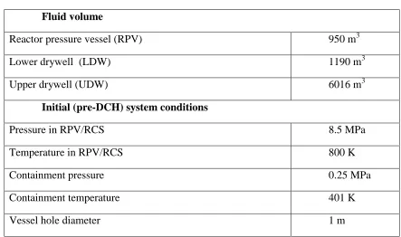
Table ‎3.1: System parameters used in simulation case study.

Fluid volume

Reactor pressure vessel (RPV) 950 m3

Lower drywell (LDW) 1190 m3

Upper drywell (UDW) 6016 m3

Initial (pre-DCH) system conditions

Pressure in RPV/RCS 8.5 MPa

Temperature in RPV/RCS 800 K

Containment pressure 0.25 MPa

Containment temperature 401 K

3.1 Description of the actual work

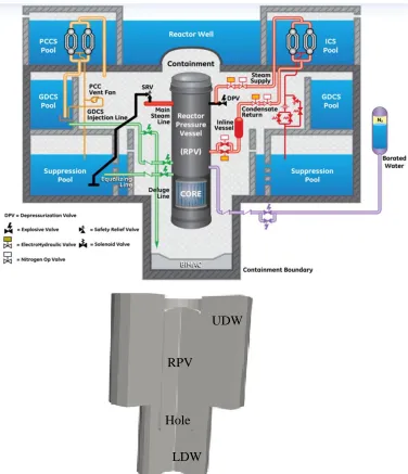
A 3D computational mesh was designed according to the data in [ 3] tabulated in Table 3.1. Figure 3.1 and Figure 3.2 depict a simplified design of an ESBWR containment and mesh designed by OpenFOAM. Since the reactor internals and many containment structures and components are not modeled, dimensions are adjusted to conserve the fluid volume. For example, the reactor pressure vessel (RPV) height is reduced to reflect the volume of reactor coolant system (RCS). While the drywell height is prototypal, the lower drywell (LDW) and upper drywell (UDW) diameter is adjusted to reflect the volume available for fluid. Suppression pool effect is not considered and the presence of the control rods and corium is not included in this initial study.

A major set of simulations was then performed with a mesh of 1.14 million nodes. The system’s total mass and total energy are checked and found to be conserved with high accuracy (0.081% and 0.56%, respectively, see Figure 3.3 and Figure 3.4. Total energy is calculated as the sum of thermal energy and kinetic energy. The simulations were performed with and without turbulence models. In the latter case, the simulations effectively use the under-resolved grid numerical diffusion as an implicit sub-grid scale turbulence model. However, the grid resolution (in case with ~1 million nodes, ) is not fine enough for capturing large eddies. The transient temperature and pressure field in the RPV, LDW and UDW are mass-averaged to obtain parameters that are compared to lumped - parameter predictions by a transient CLCH model. Appendix B illustrates some simulation snapshots for blowdown progression.

Figure ‎3.1: Computational domain (below) representing actual ESBWR containment design (above).

UDW

RPV

Figure ‎3.2: Mesh configuration: horizontal view (left) and plan view (right).

Figure ‎3.3: Change of mass during steam blowdown from reactor coolant system to containment.

0 5,000 10,000 15,000 20,000 25,000 30,000

0 4 8 12 16 20

Mass

(K

g

)

Time (second)

Reactor Coolant System Containment Lower Drywell Containment Upper Drywell Total

RPV

Figure ‎3.4: Change of total energy during steam blowdown from reactor coolant system to containment.

3.2 Model assessment

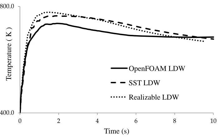
Blowdown situation involves several characteristic flow patterns such as jet flow, jet impingement, wall spreading flow and recirculation phenomena (discussed in detail in section 4.1.4 and Figure 4.6). These phenomena, individually or in combination, have been investigated in the past. Direct comparison of previous work is hindered by differences in geometry, jet to target distance, pressure ratio, Mach number, Reynolds number. This complex flow pattern requires a systematic evaluation of the CFD capability (see chapter 4). The effect of turbulence modeling on the predicted local behavior is demonstrated in Figure 3.5. Figure 3.5 compares the jet structure with data from simulation described in a previous computational work [19], where a high constant pressure boundary condition was imposed at the inlet of the nozzle and the cylinder pressure was held constant. The simulations were

0.0E+00 1.0E+10 2.0E+10 3.0E+10 4.0E+10 5.0E+10

0 4 8 12 16 20

T otal Ene rgy (J oul) Time (second)

performed using three different treatments of turbulence: no turbulence model, realizable and SST turbulence models.

In Figure 3.5, is the distance, along the jet centerline starting from the nozzle outlet center to the bottom of the containment, normalized by the nozzle diameter; is the pressure along the jet centerline normalized by the nozzle outlet center. OpenFOAM results show a good agreement with the previous results experimental results in Figure 3.5. The jet pressure distribution is the same for different pressure ratios at a given distance. For OpenFOAM simulation, because pressure ratio is not constant as there is no inlet or outlet boundary conditions, pressure ratios are calculated for any given time moment. Figure 3.6

shows that compartment-averaged pressure and temperature, particularly in the LDW, are sensitive to treatment of turbulence. For the LDW, peak temperature variation is 48.6 K.

Figure ‎3.5: Effect of overall pressure ratio on the local non-dimensional pressure profile along jet centerline.

1.0E-03 1.0E-02 1.0E-01 1.0E+00

0.01 0.1 1 10

P

/Pn

x/d Li et al, ratios 18.6 -81.4

Figure ‎3.6: LDW temperature sensitivity to turbulence models: realizable (k-ϵ)‎and‎ SST.

3.3 Simulation results

Figure 3.7 and Figure 3.8 depict OpenFOAM results and predictions by the transient version of the lumped-parameter CLCH model [ 3] with modification per Chang [ 20]. While the trends are similar between the 3D CFD simulation and the CLCH model, there remain significant differences in LDW temperature. This difference may be attributed to different discharge coefficient that causes a difference in cooling rate in the LDW. Analysis of transient fields reveals a large variation of local pressure and temperature in the LDW and UDW (Figure 3.9 and Figure 3.10). A broad range of temperature and pressure in LDW demonstrates that this variation cannot be captured by the lumped-parameter model. Given the interactions that occur locally, and depend on local pressure and temperature, the compartment-averaged quantities are unable to accurately capture the phenomena occurring at the edge of the parameter ranges.

400.0 800.0

0 2 4 6 8 10

T

emper

ature

( K

)

Time (s)

OpenFOAM LDW SST LDW

Figure ‎3.7: Comparison between OpenFOAM (SST model) results and CLCH model results. The simulation indicates an over estimate of discharge coefficient (0.85) used in the

lumped-parameter CLCH model.

Figure ‎3.8: Comparison between the OpenFOAM (SST model) results and the CLCH model results. More rapid cool down in RCS predicted by CLCH is attributed to the high

discharge coefficient.

1.0E+05 1.0E+07

0 5 10 15 20

A ve ra g e P re ssure ( pa ) Time (s) SST RCS SST LDW SST UDW CLCH_RCS

CLCH LDW & UDW

400.0 800.0

0 5 10 15

A ve ra g e T emper ature ( K ) Time (s)

SST RCS SST LDW SST UDW

Figure ‎3.9: Calculated maximum and minimum pressures for the LDW and UDW depict a wide pressure variation in the LDW.

Figure ‎3.10: Calculated maximum and minimum temperatures for the LDW and UDW depict a wide temperature variation in the LDW

1.0E+04 1.0E+05 1.0E+06

0 2 4 6

P re ssure ( pa sc al) Time (s) LDW minimum LDW maximum UDW minimum UDW maximum 250.0 550.0 850.0

0 2 4 6

4

Evaluation model development and assessment process

EMDAP is a systematic process described by NRC to assess the models used in nuclear accident calculations and to estimate and reduce uncertainty of these models. Evaluation Model (EM) is the whole framework of calculations. In our case EM includes: (i) OpenFOAM CFD solver; (ii) turbulence models; (iii) computational meshes; (iv) thermodynamic and transport properties. The following additional components are also part of EM: (v) initial assumptions; (vi) postulated scenario; (vii) initial and boundary conditions. EMDAP process consists of the following elements [ 21]:

1. Establish Requirements for Evaluation Model Capability. 2. Develop Assessment Base.

3. Develop Evaluation Model.

4. Assess Evaluation Model Adequacy.

The relation between the 4 Elements is illustrated in Figure 4.1. Steps, within each element, are described and applied to the problem under consideration in the following sections.

4.1 Requirements for evaluation model capability

Figure ‎4.1: Elements of Evaluation Model Development and Assessment [ 21].

4.1.1 Analysis purpose

In this work, steam blowdown, which is a phenomenon in DCH, is studied using CFD software package, OpenFOAM [ 4]. OpenFOAM is applied to simulate transient, multi-dimensional single-phase flow in Economic Simplified Boiling Water Reactor (ESBWR) containment in a beyond design basis accident (B-DBA). We choose to perform this

Establish requirements for evaluation model capability (1) Specify analysis purpose, transient class and power plant class. (2) Specify figures of merit.

(3) Identify systems, components, phases, geometries, fields that should be modeled. (4)Identify and rank phenomena and processes.

Develop assessment base (5)Objectives for assessment base. (6) Scaling analysis.

(7) Integral effect testing and separate effect testing to complete the

database.

(8) Evaluating effects of Integral effects distortion and separate effect scale up.

(9)Determine experimental uncertainty.

Develop evaluation model

(10) Establish EM development plan. (11) EM structure.

(12) Develop Closure Models.

simulation for ESBWR configuration, for which information and data about the containment system geometry, scenarios, and predictions are available [ 3, 22].

This study is done as a prerequisite for simulating the whole DCH scenario which is dominated by the corium energy. Corium is expected to relocate to the LDW so focus here would be on LDW phenomena which include: (i) steam blowdown, (ii) steam jet impingement and (iii) convective mixing. The suppression pool effect is not considered and the presence of the control rods and corium is not included in this initial study. A circular hole at the bottom of the pressure vessel is assumed to instantly form in the beginning of the simulation. In other words, the process of the hole ablation is ignored. Probabilities of events leading to the assumed scenarios are not considered now because the project’s goal is to assess CFD’s capability to handle such extreme scenarios.

4.1.2 Figure of merit

In a DCH scenario, spreading and entertainment of corium depend on the momentum of the blowdown steam impinging upon the corium layer. Since this study focuses on validation of CFD capability to describe the blowdown process, the Figure of Merit in this case are flow characteristics that are measured in validation experiments. Such characteristics include: (i) pressure profile along the jet centerline; (ii) Mach number along the jet centerline and (iii) Mach disk location.

4.1.3 Systems and components that should be modeled

of full geometry design and this is mostly attributed to the difficulty of simulating non symmetrical three-dimensional flows without the full geometry design (Figure 4.3 and Figure 4.4). Introduction of the additional (symmetric) constraints in highly dynamic, inherently unstable blowdown jets results in the non-physical jet behavior (Figure 4.5).

4.1.4 Phenomena identification and ranking

Development of the Phenomena Identification and Ranking Table (PIRT) aims to identify and prioritize important physical phenomena in the system/ process of interest. PIRT’s function is to ensure that we focus on the activities that will impact the figure of merit. Prioritization is derived from an importance ranking of the phenomena relative to the main requirements. Melt energy transported by steam is the main concern which is the basis for assessing the importance of simulation accuracy of any single phenomenon. PIRT also includes columns for assessing code adequacy and validation adequacy. PIRT is used to be more specific about the fidelity of our simulation. Each phenomenon has its characteristic parameters. In the following subsections we identify different phenomena and for each phenomenon, its characteristic parameters are related to the figure of merit [ 21]. Most of the interesting phenomena are demonstrated in Figure 4.6 by the numbers, which label the location of each phenomenon. To narrow down the focus of the problem, the importance of the Upper Drywell (UDW) is ranked to be low because steam role in entraining and dispersing the melt is located in the Lower Drywell (LDW).

4.1.4.1 Flow discharge

pressure so the flow velocity at the hole exit is at a sonic condition, i.e. Mach number equals one and this results in the flow choking. The pressure ratio below which flow is not choked is called the critical pressure ratio.

To identify the importance of both choked and non-choked flow, we identify the half life, as the time needed to reduce RCS pressure by 50%. Period of interest, when most of melt dispersal process occurs, is assumed to be . Initial results as shown in Figure 4.7 and Figure 4.8, reflect the uncertainty in the solver (pressure based solver and density based solver) and also in the turbulence modeling approach. In Figure 4.7, = 4 Sec or 8

Sec for laminar and turbulent flows, respectively. In Figure 4.8, of the 4 cases is

Figure ‎4.2: Systems, components, phases, geometries, fields and processes that should be modeled.

System

•ESBWR free volume ( volume available for steam)

Components

•Pressure vessel, PV Hole, Containment compartments: LDW and UDW

Phase

•Steam (gas) for blowdown and mixing processes. Containment air isn't as important as steam for this initial study.

Geometry

•Three dimensional full geometry is needed. The CFD 3D simulations were also performed for a 1/12 segment (30-degree wedge) and a ½ segment of an

axisymmetric containment. The results obtained exhibit notable differences from results of full geometry simulation. This outcome is attributed to the difficulty of introducing additional (symmetrization) constraints in highly dynamic,

inherently unstable blowdown jets.

Fields and Transport Processes

Figure ‎4.3: Different designs (from left to right): 30-degree wedge, half geometry and full scale geometry. The upper row is the top view and the lower row is the side view. Components are demonstrated on the half geometry side view. PV: Pressure Vessel. LDW and

UDW are Containment compartments: Lower Dry Well and Upper Dry Well.

At the nozzle (hole) end, the actual mass flow rate is different from the theoretical flow rate which assumes in-viscid one-dimensional ideal gas flow. The ratio of the actual discharge to the theoretical discharge is the discharge coefficient. Discharge coefficient is dependent on the nozzle shape and Reynolds number which is highly variable in our case. Therefore, we expect that discharge coefficient may be time-dependent. Accuracy of the turbulence modeling is essential to compute the correct discharge coefficient.

PV

LDW

Figure ‎4.4: Comparison between wedge, half geometry and full geometry.

4.1.4.2 Under-expanded sonic jet flow

The first flow region is the jet flow. Under-expanded jet emerges from the hole in the RPV and the expansion waves reflect at the jet boundary as compression waves. For the choked flow, the compression waves meet and form Mach disks. For lower pressure ratios, boundary reflection process does not include shocks. In both cases, jet shows a periodic behavior of the state parameters along the symmetry axis for a certain downstream distance, then the damped periodic behavior is overcome by turbulence and molecular diffusion [ 19, 23]. The global behavior of the steam can be related to jet axial parameters like Mach disk location, axial Mach number, axial pressure profile and axial velocity profile. These parameters depend on axial distance and pressure ratio.

2.0E+05 2.8E+05

0 0.04 0.08 0.12 0.16

L o w er Dr y w ell av er ag e p ress u re (p ascal) Time (sec) FullGeometry symmetryBC_wedge

Figure ‎4.6: Computation domain representing ESBWR containment design. Steam velocity is shown (Log scale) at t=1sec after blowdown initiation. Phenomena included are: 1-Flow discharge, 2- Jet flow and instability, 3-Jet impingement, 4-Wall Jet, 5- Recirculation flow,

6-Orifice Flow, 7- Mixed Convection.

6

1

4 3

2 5

Figure ‎4.7: Transient behavior of RCS pressure normalized to its initial value. Results for pressure based and density based solvers with laminar model and turbulence models (SST

and Realizable turbulence model).

Figure ‎4.8: Transient behavior of Pressure ratio. Results for pressure based and density based solvers with laminar and turbulence models. (SST: shear stress transport model and

Realizable: Realizable turbulence model). Pressure ratio is the ratio between RCS pressure to LDW pressure.

0 2 4 6 8 10

0 0.1 0.2 0.3 0.4 0.5 0.6 0.7 0.8 0.9 1 Time (sec) No rm ailze d R C S p ress u re

Pressure based laminar Pressure based SST Pressure based Realizable Density based Laminar

0 2 4 6 8

1 10 Time (sec) P ress u re ratio

4.1.4.3 Jet impingement

When the high-speed steam flow approaches the wall, its axial velocity goes to zero. As the jet slows down, kinetic energy is converted to thermal energy. The ratio between the thermal energy to kinetic energy is called the recovery factor. For highly turbulent jets ( recovery factor depends mainly on the jet - wall spacing, H normalized by nozzle diameter, d, not on the Reynolds number [ 24]. Actual and theoretical recovery factors are the same for high values of H/d (>6). Flow and temperature fields are correlated with each other. Vortices are emanating from the jet nozzle and dominating the jet close the wall. Therefore, the jet separates due to interaction between primary vortices and the wall. Jet impingement is controlled mainly by Reynolds number and jet-wall spacing [ 25, 12].

4.1.4.4 Jet instability

4.1.4.5 Wall jet

Around the wall impingement location the jet flow decelerates, turns and becomes the wall jet. The wall jet moves horizontally parallel to the wall in radial direction. As it progresses, its speed decreases as it moves away from the wall. Because the jet impingement zone is unsteady, the wall jet is also unsteady. The shear layer vortices propagate into the wall jet. Moving away from the nozzle, the jet thickness increases. This thickness is evaluated by measuring the height at which the wall parallel velocity drops to 50% of the maximum radial speed of the wall jet. Wall jet properties are reported as a function of pressure ratio and nozzle/plate distance, H/d [ 26].

4.1.4.6 Recirculation flow

Interaction between the wall jet and the confinement surface creates a recirculation zone (big vortex). This zone is not noticed when studying free jets. The effect of Reynolds number on this zone is negligible. When the aspect ratio (cylinder height to its diameter) increases, the vortex length increases and its location moves downstream. Lower aspect ratio means that the wall jet is affected by the confinement surface close to the jet centerline so smaller vortex is produced [ 27].

4.1.4.7 Fluid properties

decrease and temperature decrease were reported before [ 19, 28 ]. For steam, this decrease in pressure and temperature to values lower than the initial pressure and temperature results in condensation and appearance of the liquid phase. This may reduce the high speed and high momentum of the jet.

4.1.4.8 Geometry impact

To ESBWR, pressure vessel bottom is penetrated by control rods and control rod drive. Therefore, steam blowdown consequences are probably overestimated because control rods are expected to hinder the jet flow. On the other hand, high temperature melt relocation at the lower plenum and ejection to the containment threatens the attachments of control rods. Therefore the assumption of control rod absence is quite feasible.

4.1.4.9 Orifice flow

The path between Lower Drywell and Upper Drywell is constricted by 8 large blocks which support the pressure vessel. Thus, 70% of the flow path between LDW and UDW is occupied [ 3]. This sudden reduction in cross sectional area would increase steam velocity and reduce its static pressure. Steam momentum at UDW and melt energy transport to UDW will be impacted by that constriction.

4.1.4.10Mixed convection

steam stratification is unstable and thus results in mixing. Therefore heat is transferred, at UDW, by both pressure forces and buoyant forces. Natural convection spread the melt energy at the containment, however; this research focuses on melt entrainment and dispersion by highly energetic steam so low ranking is given to UDW natural convection.

4.1.4.11 Steam condensation

Fluid at Upper Drywell is initially less hot than hot steam at lower drywell. Therefore a fraction of steam may condense at UDW. The steam condensation rate is probably slow relative to the highly dynamic steam blowdown. Therefore condensation won’t impact direct containment heating accident. Finally, all these phenomena are tabulated and ranked in Table 4.1.

4.2 Development of the assessment base

Table ‎4.1: Phenomena Identification and Ranking Table.

Since the steam blowdown process occurs with high pressure gradient where the compressibility effects are important, the validation is done using OpenFOAM compressible solvers. Three different solvers are tested [ 4]:

1. sonicFoam: This is a transient pressure-based solver for trans-sonic/supersonic gas flow. It is considered because of the high ranking given to the sonic jet flow as explained previously.

2. rhoCentralFoam: This is a density-based compressible flow solver.

3. compressibleMultiphaseInterFoam: This solver is designed for two or more

compressible fluids using volume of fluid phase fraction-based interface capturing approach. It is suitable for simulating the whole DCH phenomena.

Module Phenomena and effects Rank

PV Flow discharge Choked flow H

Non-choked flow L

LDW

Jet flow H

Jet impingement H

Jet instability H

Wall jet H

Recirculation H

Fluid properties H

Geometry impact L

UDW

Orifice flow L

Mixed convection L

4.2.1 Jet impingement and wall jet problem

First validation experiment is the jet impingement followed by wall jet as described in [29]. Subsection ( A) gives a description of the problem and the problem setup. CFD capability is then evaluated by comparing numerical results to experimental data using different turbulence models and different OpenFOAM solvers in subsection ( B). Conclusions and insights gained from the results are summarized in subsection ( C).

A. Description

Figure 4.9 shows the turbulent jet discharged from a circular nozzle and then impinging on the bottom wall. The jet nozzle diameter, d, is 0.01m. The jet Reynolds number is 23,000 (based on the jet velocity, diameter and fluid viscosity). The distance from the jet nozzle to the impingement plate, H, is 6 nozzle diameters, ( ). Jet centerline to outlet distance is 20d (far from the jet to avoid the effect of the outlet boundary condition on the results). The simulation is done initially with non-uniform three dimensional meshes which are refined in the radial direction around the jet, Figure 4.10. The adopted grid size for initial computations is 104 (radial) × 90 (normal to the plate). Experimental data are given in terms of the bulk velocity of the nozzle so the inlet section is designed to be outside the main domain at the distance of half the nozzle diameter. This added nozzle helps to introduce more realistic turbulent velocity profile at the nozzle exit, Figure 4.11.

The boundary conditions are as follows: Pressure: Zero gradient at all the boundaries.

Velocity: Inlet velocity is 35.6 m/s, equivalent to the jet Reynolds number, 23,000. No slip (zero velocity) boundary condition is imposed at the walls. Boundary condition at the outlet: zero gradient. The width of the domain is large enough so the simulation results obtained at the central part of the domain are not sensitive to the outlet boundary condition.

Turbulence parameters ( ): Turbulent inflow conditions were calculated based on inlet velocity and low turbulence intensity, Turbulence intensity is defined as

( 4-1)

Figure ‎4.9: Velocity profile for impinging jet.

Figure ‎4.10: Mesh configuration used for simulating jet impingement. Impingement wall

Ou

tlet

Inlet

Impingement Wall

Wall

Ou

Figure ‎4.11: Velocity profile at the nozzle exit.

Zero gradient boundary condition is imposed on the wall and outlet boundaries except for the high Reynolds number Realizable model which requires imposing a wall function at the wall. Inlet values of are calculated from the following equations [11]:

_{( 4-2)}

( 4-3)

_{( 4-4)}

( 4-5)

, , the velocity fluctuations in the directions respectively. : the turbulence intensity

inlet velocity 0 5 10 15 20 25 30 35 40

0 0.002 0.004 0.006 0.008 0.01

Velo city m ag n itu d e ( m /s )

, an empirical constant : the length scale

: the characteristic length (nozzle diameter). The initial conditions are as follows:

Pressure: 1 bar Temperature: 300 K Velocity: zero

Turbulence parameters ( ): Initially, there is no turbulence (zero values).

Thermodynamic properties: Constant thermodynamic coefficients of air, with a specific heat capacity J/ (kg· K); Prandtl number and dynamic viscosity _{Kg/ (m.s).}

Time Step: Maximum Courant number was set to be 1.0 so time step is variable but it stabilizes around . Courant number, , is defined in terms of velocity magnitude, time step, and length interval.

( 4-6)

B. Solver evaluation

models for compressible fluids. The following turbulence models has been tested: Shear Stress Transport model (SST) [ 18] Realizable Model [ 16], Launder & Sharma Model [ 15]. More details about these models are in subsection 2.2.

Figure 4.13 depicts the variation of the average velocity at the symmetry axis as the jet approaches the impingement plate. is the height above plate. Average axial velocity, is normalized by bulk velocity ( ). Bulk velocity is calculated according to the following equation [29]:

( 4-7) where is the bulk velocity, is the centerline velocity, is the Reynolds number.

We note that the three models follow the general trend of the experimental data. SST model and Realizable perform better than Launder and Sharma model and give approximately the same results at y/d <0.5 and y/d >1.5. SST model gives better results than the other 2 models, especially in the region where: 1.4> y/d >0.5.

Figure ‎4.12: Velocity change with time at a point which is labeled (on the right).

0.0 1.0 2.0 3.0 4.0 5.0 6.0 7.0

0 0.01 0.02 0.03 0.04 0.05

Velo

city

(

m

/s

)

Figure ‎4.13: Mean velocity normal to the wall computed by SST, Launder and Sharma and realizable turbulence models.

The near-wall behavior is demonstrated in Figure 4.14 which shows the absolute values of the velocity very close to the wall. It is notable that the experimental mean velocity does not go to zero near the wall. In reference [ 29] this was attributed to the fact that when the mean velocity approaches zero, the measurement signal is more affected by the turbulent fluctuating velocity near the wall. Assuming that the velocity fluctuations, , (radial and axial) are isotropic, velocity, , was corrected to be , in the same reference, by the equation:

( 4-8)

This correction reduces the mean velocity near the wall and negligibly influences the results far from the wall. In Figure 4.14, velocity calculations based on SST model come between the experimental velocity and the corrected velocity.

0 0.2 0.4 0.6 0.8 1 1.2

0 0.5 1 1.5 2 2.5 3

Velo city n o rm alize d b y b u lk v elo city ( u /U b )

Axial distance normalized by nozzle diameter (y/d) Experiment SST

The Wall jet

The turbulent wall jet is the jet reflected by a wall and extends to the other side as it can be seen in Figure 4.9. The wall jet consists of two layers. The inner layer is similar to the boundary layer. The outer layer is like a free shear flow. Figure 4.15 is a diagram of the typical wall jet which is characterized by the jet half width, , which is the location

where . is the radial velocity and is the maximum radial velocity in wall jet.

Figure ‎4.14: Near wall axial mean velocity.

To assess the CFD calculations for the turbulent wall jet growth and spreading, radial growth of jet half width computed with OpenFOAM is compared with experimental results in reference [29].

0.0 0.5 1.0 1.5 2.0 2.5 3.0 3.5 4.0 4.5 5.0

0 0.01 0.02 0.03 0.04 0.05

Velo

city

(

m

/ sec)

Axial distance normalized by nozzle diameter (y/d) Experimental

In Figure 4.16, the experimental radial wall jet grows linearly with radial distance. It is noted that both Low Reynolds Number turbulence models (SST and Launder and Sharma) capture (over-predict) the wall jet growth. Realizable turbulence model does not simulate the jet growth. Difference in wall jet growth between the calculations of the three turbulence models is shown in Figure 4.17.

Figure ‎4.15: Fully developed velocity profile of a wall jet [ 30].

Figure ‎4.16: Radial Growth of jet half width.

Launder & Sharma Model

SST Model Realizable Model

Figure ‎4.17: Radial wall jet as expected by different turbulence models.

0 0.2 0.4 0.6

2 2.5 3 3.5 4 4.5 5

W all Jet Half T h ick n ess n o rm alize d b y n o zz le d iam eter (y1/ 2 /d )

Radial distance normailzed by nozzle diameter (r /d)

Experimental

SST

Launder and Sharma

Performance of different solvers

All the previous results were obtained with the pressure-based solver, sonicFoam. The next solver to be tested is the compressible density based solver, rhoCentralFoam. To stabilize the solver, we had to decrease the maximum Courant number from 1 to 0.25. This led to increasing the simulation cost by a factor of 83 times so rhoCentralFoam solver was deemed to be too computationally expensive for this case. The simulation cost of the third solver, compressibleMultiphaseInterFoam, is 2.5 times more expensive than sonicFoam.

Figure 4.18 shows the variation of the average velocity at the symmetry axis as jet approaches the impingement plate calculated by both sonicFoam and compressibleMultiphaseInterFoam (using the same mesh and boundary conditions). For both

solvers, SST turbulence model is used and the maximum Courant number is 1.0. Both solvers give the same trend, but sonicFoam give better results with less expensive simulation. This includes both Courant number effect and slower performance per iteration. One has to keep in mind that the second solver also has the multiphase flow simulation capability which is relevant to the problem of interest in this work.