Earth Planets Space,50, 501–505, 1998
Three-dimensional infrared models of the interplanetary dust distribution
S. M. Kwon1and S. S. Hong2
1Department of Science Education, Kangwon National University, Chunchon, Korea 2Department of Astronomy, Seoul National University, Seoul, Korea (Received December 8, 1997; Revised April 9, 1998; Accepted April 13, 1998)
We have calculated the brightness of zodiacal emission by using the three dimensional optical models of zodiacal cloud. By comparing the calculated brightness distribution with theIRASobservations, we found that the cosine model is the best out of the three for describing the helioecliptic latitude dependence of dust distribution. We also found best parameters for the heliocentric variations of the dust temperature and volumetric absorption cross-section. Inclination and ascending node of the symmetry plane were deduced from annual variations of i) the peak offset latitude and ii) the pole brightness difference. Longitudes of the ascending node derived from i) and ii) are shown to be significantly different from each other.
1.
Introduction
On the basis of visible zodiacal light (ZL), many models have been constructed for the three dimensional distribution of dust particles in the zodiacal cloud (Gieseet al.(1986) and references therein). Although most models agree in that the density decreases by a factor of 2 within 0.2 to 0.3 AU above the Earth orbit (Giese and Kneißel, 1989), the result-ing morphology of the isodensity contours in the helioecliptic meridian looks quite different from model to model. Bright-ness distribution of the zodiacal emission (ZE) obtained by the IRAS(Hauser and Houck, 1986) may discriminate the models from each other.
2.
Model Calculations
2.1 IR brightness integral
To obtain the ZE brightness at wavelengthλ, we numeri-cally calculate the following IR brightness integral:
Z(−, β;λ)= ∞
0
n(r, β)σabs(r, λ)Bλ[T(r)]dl, (1)
wheren(r, β)denotes the dust number density at position (r, β),σabs(r, λ)is the mean absorption cross-section of the
dust particles, andBλ[T(r)] means the Planck function eval-uated with average temperatureT(r)of the particles at dis-tancer from the Sun. As shown in Fig. 1, the heliocentric latitudeβis measured from the symmetry plane. By calling βthe heliocentric symmetry-plane latitude we distinguish it
from the heliocentric ecliptic latitudeβ◦and from the usual geocentric ecliptic latitudeβ. Inclination angle of the sym-metry plane is denoted by i, the angle η orients the line of nodes of the plane with respect to the Sun-Earth direc-tion, andφis the heliocentric longitude of(r, β)measured from the same direction. These angles satisfy the relation sinβ=cosβ◦−sinicosβ◦sin(η+φ).
Copy right cThe Society of Geomagnetism and Earth, Planetary and Space Sciences (SGEPSS); The Seismological Society of Japan; The Volcanological Society of Japan; The Geodetic Society of Japan; The Japanese Society for Planetary Sciences.
In most analyses of the ZL observations an expression of the formn(r)f(β)is used to portray the three dimensional distribution of the dust particles. The functionn(r)is for heliocentric distribution, herer being measured in the sym-metry or the ecliptic plane; while f(β)describes distribution over the heliocentric symmetry-plane latitude. As an approx-imation forn(r)one often adopts a power law relation of the form
n(r)=n◦ r
◦
r ν
, (2)
wheren◦ is the number density at a reference distance r◦, for which 1 AU is usually taken (cf. Leinertet al., 1981). A variety of models have been proposed for f(β). Among them are the ellipsoid model f(β)=[1+(6.5 sinβ)2]−0.65
by Giese and Dziembowski (1969), the fan model f(β)= exp[−2.1|sinβ|] by Leinertet al. (1981), and the cosine model f(β)=0.15+0.85 cos28βby Rittich (1986).
The model parameters were fixed at the values suggested by the authors of each model and were not changed during the calculations of ZE. By doing so, we could check com-patibility of the optical 3-dimensional models with theIRAS observations of zodiacal emission. Hong and Kwon (1991) showed that the ellipsoid model is in an accordance with the Gegenschein part of the visible ZL. In analyses of the in-frared ZE, however, many investigators (Hauseret al., 1985; Murdock and Price, 1985; Deul and Wolstencroft, 1988; and Rowan-Robinsonet al., 1990) preferred fan-type models. It is then interesting to see which of the optical models is in agreement with the ZE observations.
We let a power law of indexδ
T(r)=T◦ r◦
r δ
(3)
describe the variation of dust temperature withr. Here,T◦ de-notes the dust mean temperature at the Earth orbit. Since it is hard to de-couple radial dependence of the dust number den-sity from that of the absorption cross-section, we simply as-sign to the volumetric absorption cross-sectionn(r)σabs(r, λ)
Fig. 1. Geometry involved in the IR brightness integral.
a power law relation of another index:
ζ(r;λ)≡n(r)σabs(r, λ)=ζ◦(λ)
r
◦
r γ
, (4)
whereζ◦(λ)denotes its value at the earth orbit. 2.2 IR brightness distribution in the ecliptic plane
If optical properties of various dust species and their mix-ing ratios are uniform over interplanetay space and the total number density follows a single power law relation, then the indicesγ,νandδall become constants ofr. However, many studies (for example, Hong and Um (1987), Hong and Kwon (1988), Temiet al. (1989), and Levasseur-Regourd and Dumont (1990)) indicate that power law relations with
fixed indices are inadequate for the ZE observations. In this study we will have aflexibility of varying bothγ andδwith heliocentric distance. For the volumetric absorption cross-section we take
γ (r)=γ◦−γ π tan−1(
r−r◦
AU ) (5)
withγ◦ =1.0 and for the dust mean temperature withδ◦= 0.4
δ(r)=δ◦+δ π tan−
1(r−r◦
AU ). (6)
The brightness distributions of the ZE at 12 and 25μm were calculated by integrating Eq. (1), with Eqs. (5) and (6) being substituted forγ andδ, respectively. By comparing the calculated distributions in the ecliptic plane with theIRAS
observations, one may determine the best values for the pa-rametersγ,δ, and twoζ◦’s.
There are calibration differences among the different ver-sions of the Zodiacal Observations History File (ZOHF) (Vrtilek and Hauser, 1995). In the comparison done in Fig. 2 we have used the ZOHF release 2, which was also used
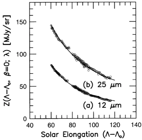
Fig. 2. Distribution of the IR brightness with differential solar elongation. TheIRASdata (open circles) at (a) 12μm and (b) 25μm are compared with the model calculations (solid lines).
by Reach (1991). The best parameter values are γ = 0.6, δ = 0.3, and ζ◦(12 μm) = 9.7×10⁻²¹ cm−1 and
S. M. KWON AND S. S. HONG: INTERPLANETARY DUST DISTRIBUTION 503
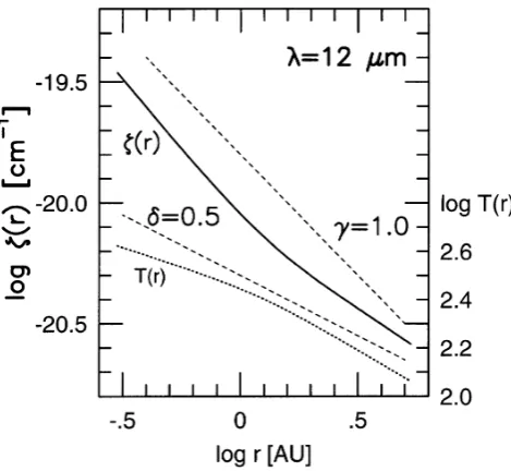
Fig. 3. Heliocentric variations ofζ(r)at 12μm andT(r)are shown for the best-fit indices ofγ (r)andδ(r). Single power-law relations with γ=1.0 andδ=0.5 are shown by dashed lines for comparison.
than 0.5 up to 3 AU, and the gradient slowly reaches its lim-iting value 0.55 atr 8 AU. The volumetric absorption cross-sectionζ(r)varies more steeply within the Earth orbit than beyond it.
2.3 IR brightness distribution off the ecliptic plane We are now tofind out best models for the distribution of density over heliocentric symmetry-plane latitude. For each of the three optical models, we integrated Eq. (1) with
−fixed at 90◦andβvarying from−90◦to 90◦. Details of the brightness profile overβdepend on the orientation of the symmetry plane, which enables us to locate the symmetry plane in terms ofi and.
The calculated brightness profiles over the helioecliptic meridian are directly compared, in Fig. 4, with the corre-spondingIRAS(thick solid lines) observations at 12μm and 25μm. In thefigure the dotted, solid, and dashed lines are for the cosine, fan, and ellipsoid models, respectively. Out of the three the cosine model delivers, in an overall sense, the best agreement with theIRASobservations.
The brightness profiles from the fan model show sharp peaks near the symmetry plane and broad wings towards the ecliptic poles. And the pole brightness at 25μm shows an excess of∼7 MJy/sr over the observed value. The profiles from the ellipsoid model do not have such peaks near the symmetry plane, and are very similar to the ones from the cosine model in the range−20◦ⱗβⱗ20◦. However, it also shows a significant excess of brightness towards the poles.
3.
Symmetry Surface
It has been known that the surface of maximum dust den-sity does not coincide with the ecliptic plane. We usually call the maximum density surface the symmetry plane, under the notion that it would form a plane. If it is a plane, one set ofi anduniquely locates the surface with respect to the ecliptic plane. Many investigators deduced thei andsets from the ZL and ZE observations. (See the references in
Ta-ble 1 and some recent discussions by Ishiguroet al. (1996) and Dermott et al. (1997).) As can be seen from Table 1, the results depend on the data and the deduction method. This conflicting situation was interpreted as an indication of warped nature for the maximum density surface (Misconi, 1980; Vrtilek and Hauser, 1995). We also assume a planar surface, not because the maximum density surface is planar, but because an accumulation ofiandsets would eventually help us define its nature.
The ZL or ZE profile over β, at a fixed elongation say 90◦, shows its maximum not necessarily at β = 0. The peak occurs slightly off the ecliptic plane. If the maximum density surface forms a plane, the offset amount would vary sinusoidally with time of the year. A monitoring of the peak latitude βpeak over a year would determine i and . The difference in brightness between the north and south ecliptic poles would also show a sinusoidal variation with time. The
IRAShas in fact done such monitorings.
We have numerically generated a series of ZE profiles over
βand determinedβpeakas a function ofη. As far as the peak brightness latitude is concerned, the f(β)models are of no consequences. By comparing the resulting run ofβpeakwith the 12μm data of ZOHF release 2, we were able tofixiand 59◦. The discrepancy is due to the difference in comaprison data; our result based on the ZOHF release 3 agrees with theirs.
A run of the pole brightness difference was also made from the generated profiles, and compared with the IRAS
observations of ZHOF release 2. The solid, dashed, and dotted lines in Fig. 6 are from the cosine, ellipsoid, and fan models, respectively. Equally good fits were made by the cosine and the ellipsoid models with the same set of i =
2.◦3±0.◦1 and=75◦±2◦. As can be seen from thefigure, the cosine and ellipsoid models are hardly distinguishable from each other. However, the fan model differs from the other two. The comparison done with the ZOHF release 3 gave us the same=75◦±2◦, but the inclination value was reduced toi =1.◦9±0.◦1. Using the same ZOHF release 3, Vrtilek and Hauser (1995) placed the ascending node at= 76.◦1, but with the method based on geometricalfitting they could not determine the inclination value.
Phase of the annual variation curve for the pole brightness difference is solely determined by; while its amplitude is controlled by the column densities along the two directions of ecliptic poles. Therefore, the amplitude should depend on the model of f(β)and the inclination as well. For a given model of f(β), the larger the observed amplitude is, the higher the derived i should be. This enables us to discriminate the three dimensional models of density from each other. This is also why the two sets of ZOHF yield different values for the inclination.
Fig. 4. The ecliptic latitude profiles (thick solid lines) of theIRASbrightness observed at (a) 12μm and (b) 25μm are compared with the results (dotted lines) from the best-fit cosine model. The results from the fan (thin solid lines) and the ellipsoid (dashed lines) models are also given for comparison.
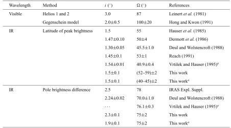
Table 1. Variousiandvalues for the symmetry plane.
Wavelength Method i(◦) (◦) References
Visible Helios 1 and 2 3.0 87 Leinertet al.(1981)
Gegenschein model 2.0±0.5 100±20 Hong and Kwon (1991)
IR Latitude of peak brightness 1.5 55 Hauseret al.(1985)
1.47±0.10 50±4 Dermottet al.(1986)
1.30±0.05 45.5±1.0 Deul and Wolstencroft (1988)
1.45±0.1 53±1 Reach (1991)
1.54±0.01 40.9±0.4 Vrtilek and Hauser (1995)a
1.5±0.1 (52–59)±2 This work
1.5±0.1 (40–45)±2 This worka
IR Pole brightness difference 2.5 78 IRAS Expl. Suppl.
2.24±0.02 70.0±1.0 Deul and Wolstencroft (1988)
· · · 76.1±0.3 Vrtilek and Hauser (1995)a
2.3±0.1 75±2 This work
1.9±0.1 75±2 This worka
aObtained from the release 3.0 of ZOHF.
brightness diffference. But the two set of results from the peak offset and the pole brightness difference do not agree with each other, particularly for the longitude of ascending node.
4.
Conclusion and Discussion
We have seen that the change of mean dust temperature with heliocentric distancercan not be described by a power law of single exponent. The raidal change in the exponent
δ(r)as given in Eq. (6) suggests that mean dust properties vary systematically with distance from the sun. If multi-species nature is accepted for the zodiacal dust particles (Hong and Um, 1987; Hong and Kwon, 1988; Levasseur-Regourd and Dumont, 1990; Kneißel and Mann, 1991; Reach, 1991), this kind of systematic variation can be an indication of changing mixture ratios.
S. M. KWON AND S. S. HONG: INTERPLANETARY DUST DISTRIBUTION 505
Fig. 5. The observed annual variation of the peak brightness latitude is compared with that from the model calculation. The leading scans (open circles) at 12μm arefitted withi=1.◦5 and=59◦(solid line); while the trailing ones (filled circles) are withi =1◦.5 and=52◦(dotted line).
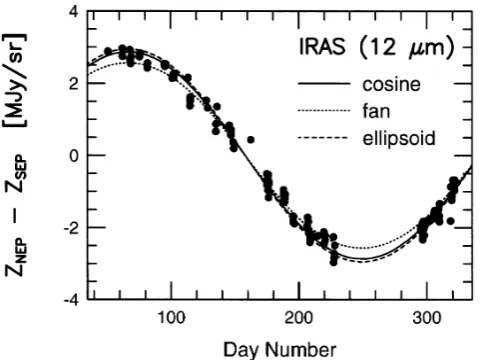
Fig. 6. Annual variation of the pole brightness difference at 12μm isfitted to the model calculation withi=2.◦3 and=75◦. The bestfit line (solid one) is from the cosine model. The dashed line is from the ellipsoid model and dotted from the fan one.
goodfits to the ZE data can be made by the ellipoid model, but bestfits are done with the cosine model. This doesn’t necessarily mean an existence of the central halo portrayed by the cosine model, because we haven’t analysed inner parts of the zodiacal emission yet.
Acknowledgments. SSH was supported in part by the Korean Min-istry of Education, Basic Science Research Institute grant No. BSRI-97-5411, and SMK by the travel fund of Kangwon National
Uni-versity, Republic of Korea.
References
Dermott, S. F., P. D. Nicholson, and B. A. Wolven, Preliminary analysis of the IRAS 1. Solar System dust data, inAsteroids, Comets, Meteors II, edited by C.-I. Lagerkvist, B. Lindblad, H. Lundstedt, and H. Rickman, 583pp., HSC, Uppsala, 1986.
Dermott, S. F., K. Grogan, E. K. Holmes, and S. J. Kortenkamp, The dynam-ical structure of the zodiacal cloud, paper presented at ZCS workshop, Kobe, 1997.
Deul, E. R. and R. D. Wolstencroft, A physical model for thermal emission from the zodiacal dust cloud,Astron. Astrophys.,196, 277–286, 1988. Giese, R. H. and C. V. Dziembowski, Suggested zodiacal light measurements
from space probes,Planet. Space Sci.,17, 949–956, 1969.
Giese, R. H. and B. Kneißel, Three-dimensional models of the zodiacal cloud: II. Compatibility of proposed infrared models,Icarus,81, 369– 378, 1989.
Giese, R. H., B. Kneißel, and U. Rittich, Three-dimensional models of the zodiacal dust cloud: A comparative study,Icarus,68, 395–411, 1986. Hauser, M. G. and J. R. Houck, The zodiacal background in the IRAS data,
inLight on Dark Matter, edited by F. P. Israel, 39pp., Dordrecht, Reidel, 1986.
Hauser, M. G., T. N. Gautier, and F. J. Low, IRAS observations of the inter-planetary dust emission, inProperties and Interactions of Interplanetary Dust, edited by R. Giese and P. Lamy, Reidel, Dordrecht, 43pp., 1985. Hong, S. S. and S. M. Kwon, Connection between the infrared zodiacal
emission and the visible zodiacal light,Vistas in Astronomy,31, 11–21, 1988.
Hong, S. S. and S. M. Kwon, On the gegenschein and the symmetry plane, in Origin and Evolution of Interplanetary Dust, edited by A. C. Levasseur-Regourd and H. Hasegawa, 147pp., Kluwer, Dordrecht, 1991. Hong, S. S. and I. K. Um, Inversion of the zodiacal infrared brightness
integral,Astrophys. J.,320, 928–935, 1987.
Ishiguro, M., R. Nakamura, T. Watanabe, T. Mukai, H. Tanabe, I. Mann, H. Kimura, P. Hillebrand, and J. F. James, North-south asymmetry of the zodiacal light, inProc. of the 29th ISAS Lunarand Planetary Symposium, edited by H. Mizutani, 64pp., ISAS, Kanagawa, 1996.
Kneißel, B. and I. Mann, Spatial distribution and orbital properties of zodi-acal dust, inOrigin and Evolution of Interplanetary Dust, edited by A. C. Levasseur-Regourd and H. Hasegawa, 139pp., Kluwer, Dordrecht, 1991. Leinert, C., I. Richter, E. Pitz, and B. Planck, The zodiacal light from 1.0 to 0.3 A.U. as observed by the Helios space probes,Astron. Astrophys., 103, 177–188, 1981.
Levasseur-Regourd, A. C. and R. Dumont, IRAS observations and local properties of interplanetary dust,Adv. Space Res.,10, (3)163–(3)170, 1990.
Misconi, N. Y., The symmetry plane of the zodiacal cloud near 1 AU, inSolid Particles in the Solar System, edited by I. Halliday and B. A. McIntosh, 49pp., Dordrecht, Reidel, 1980.
Murdock, T. L. and S. D. Price, Infrared measurements of the zodiacal light, Astron. J.,90, 375–386, 1985.
Reach, W. T., Zodiacal emission II. Dust near the ecliptic,Astrophys. J., 369, 529–543, 1991.
Rittich, U., Die raumliche Verteilung des Interplanetaren Staubes: Mod-¨ ellrechnungen zur Interpretation von Zodiakallichtmessungen,Diploma Thesis, Ruhr University, Bochum, 1986.
Rowan-Robinson, M., J. Hughes, K. Vedi, and D. W. Walker, Modelling the IRAS zodiacal emission,MNRAS,246, 273–278, 1990.
Temi, P., P. De Bernardis, S. Masi, G. Moreno, and A. Salama, Infrared emission from interplanetary dust,Astrophys. J.,337, 528–535, 1989. Vrtilek, J. M. and M. G. Hauser, IRAS measurements of diffuse solar system
radiation: Annual sky brightness variation and geometry of the interplan-etary dust cloud,Astrophys. J.,455, 677–692, 1995.