High-accuracy statistical simulation of planetary accretion: I. Test of the accuracy
by comparison with the solution to the stochastic coagulation equation
Satoshi Inaba1, Hidekazu Tanaka1, Keiji Ohtsuki2, and Kiyoshi Nakazawa1
1Department of Earth and Planetary Sciences, Faculty of Science, Tokyo Institute of Technology, Tokyo 152-8551, Japan 2Computing Service Center, Yamagata University, Yamagata 990-8560, Japan
(Received September 22, 1998; Revised February 10, 1999; Accepted February 12, 1999)
The object of this series of studies is to develop a highly accurate statistical code for describing the planetary accumulation process. In the present paper, as a first step, we check the validity of the method proposed by Wetherill and Stewart (1989) by comparing the results obtained by their method with the analytical solution to the stochastic coagulation equation (or to a well-evaluated numerical solution). As the collisional probability Ai j
between bodies with masses ofi m1andj m1(m1being the unit mass), we consider the two cases: one isAi j∝i×j and another is Ai j ∝ min(i,j)(i1/3+ j1/3)(i + j). In both cases, it is known that runaway growth occurs. The
latter case corresponds to a simplified model of the planetesimal accumulation. We assumed that a collision of two bodies leads to their coalescence. Wetherill and Stewart’s method contains some parameters controlling the practical numerical computation. Among these, two parameters are important: the mass division parameterδ, which determines the mass ratio of the adjacent mass batches, and the time division parameter, which controls the size of a time step in numerical integration. Through a number of numerical simulations for the case of Ai j =i×j, we find that whenδ≤1.6 and≤0.03 the numerical simulation can reproduce the analytical solution within a certain level of accuracy independently of the size of the body system. For the case of the planetesimal accumulation, it is shown that the simulation withδ ≤ 1.3 and ≤ 0.04 can describe precisely runaway growth. Because the accumulation process is stochastic, in order to obtain reliable mean values it is necessary to take the ensemble mean of the numerical results obtained with different random number generators. It is also found that the number of simulations,Nc, demanded to obtain the reliable mean value is about 500 and does not strongly depend on the functional form of Ai j. From the viewpoint of the numerical handling, the above value ofδ(≤1.3)andNc(∼500) are reasonable and, hence, we conclude that the numerical method proposed by Wetherill and Stewart is a valid and useful method for describing the planetary accumulation process. The real planetary accumulation process is more complex since it is coupled with the velocity evolution of the planetesimals. In the subsequent paper, we will complete the high-accuracy statistical code which simulate the accumulation process coupled with the velocity evolution and test the accuracy of the code by comparing with the results ofN-body simulation.
1.
Introduction
The numerical simulations of the planetary accumulation process have been so far investigated by two different ways: the N-body simulation and the statistical approach based on the Smoluchowski equation. In theN-body simulation (e.g., Lecar and Aarseth, 1986; Beaug´e and Aarseth, 1990; Aarsethet al., 1993; Kokubo and Ida, 1996) orbits of bodies are directly integrated by taking into account coalescences between them. Because of the limitation of computational ability, the number of the bodies treated in this technique is limited to only about 10000 bodies at most. However, in the early stage of the planetesimal accumulation, the number of planetesimals is inferred to be of the order of 1010 to 1012 (Greenberget al., 1978; Hayashiet al., 1985). Even in the late stage of planetary accumulation, destructive collisions between planetesimals would create a large number of frag-ments. Thus, it is clear thatN-body simulation cannot cover the whole process of the planetary accumulation though it is
Copy right cThe Society of Geomagnetism and Earth, Planetary and Space Sciences (SGEPSS); The Seismological Society of Japan; The Volcanological Society of Japan; The Geodetic Society of Japan; The Japanese Society for Planetary Sciences.
a powerful method under some suitable conditions.
In the stage where a huge number of bodies exist, it is necessary to introduce a statistical approach of some kind. In a statistical approach (e.g., Safronov, 1969; Greenberg
et al., 1978; Nakagawaet al., 1983; Ohtsukiet al., 1988),
we usually describe the body system by the Smoluchowski equation which is expressed as (Smoluchowski, 1916)
d Nk
dt =
1 2
i+j=k
Ai jNiNj−Nk
∞
i=1
Ai kNi, (1)
where Nk is the number (or the number density) of bodies with masskm1(m1being a unit mass and, from now on, put to be unity) and Ai j is the collisional probability between bodies with massesi and j. In a planetesimal accumula-tion process, the collisional probabilityAi jis the function of the relative random velocity between the planetesimals with massi and j and, thus, the velocity evolution of planetes-imals must be calculated simultaneously with the accumu-lation process. Since the statistical approach is based on a number of assumption (e.g., spatially homogeneous distribu-tion of planetesimals), the validity of the statistical approach is not clear. Hence, the validity of the statistical approach
should be investigated, for example, by the comparison with
N-body simulations.
Furthermore, though the Smoluchowski equation seems to be rational, it is known that the Smoluchowski equation breaks down in cases of runaway growth (e.g., for a colli-sional probabilityAi j =i×j). In runaway growth, relatively large bodies grow faster than other smaller bodies because of strong positive dependence of the collisional probability on masses of bodies (Greenberget al., 1978; Wetherill and Stewart, 1989; Barge and Pellat, 1991; Spauteet al., 1991; Kokubo and Ida, 1996). Such rapidly growing bodies in the high mass end of the mass distribution are called runaway bodies. Even among the runaway bodies, larger bodies grow faster than smaller ones andfinally, one or a few bodies grow prominently, i.e., runaway growth of a few bodies occurs. Such a mode of the accumulation process cannot be intrin-sically described by the Smoluchowski equation because it stands on the assumption that there exist a sufficiently large number of bodies in each relevant mass range. Hence, it is necessary to introduce a new statistical approach if we try to describe precisely runaway growth.
A more basic equation, which is valid in all types of the accumulation processes, was derived by Marcus (1968) in the field of atmospheric sciences. In his formulation, the accumulation process is regarded as a Markov process and a set of the body numbers in all mass bins{ni}is consid-ered as a random variable whereni is the number of bodies with massi. His equation is the time development equation of the probability with which the body system is in a state
{ni}. Bayewitzet al.(1974) and Lushnikov (1978) solved this equation analytically in the cases ofAi j=1 andAi j =i+j, i× j, respectively. On the other hand, in thefield of plan-etary sciences, Tanaka and Nakazawa (1993) independently derived the same equation (they called it the stochastic coag-ulation equation) and found analytical solutions in the cases of Ai j =1,i+j, andi× j. Tanaka and Nakazawa (1994) also showed that, for the three cases ofAi jmentioned above, the Smoluchowski equation can approximately describe the number of bodies in each mass bin as long as the body mass is much smaller than a certain critical mass which depends on the functional form ofAi j. Although the stochastic coagula-tion equacoagula-tion gives an exact picture of the accumulacoagula-tion pro-cess, it is hopelessly difficult to solve this equation for other general cases of Ai j even by numerical procedures because it is quite difficult to cover all possible states{ni}perfectly.
Thus, it is unsuitable to apply this equation to study of the real accumulation process.
Wetherill and Stewart (1989) developed an alternative nu-merical approach (this nunu-merical method will be called WS89 method in the present paper) which supplements the defects of the Smoluchowski equation. This method were presented in more detail in Wetherill (1990). In the Smolu-chowski equation the number of bodies Ni becomes a frac-tional value though the number of bodies should be, of course, an integer. To avoid this defect, in WS89 method the num-ber of collisions during each numerical time step is forcely assigned to be an integer by the Monte Carlo method when the number of collisions is a fractional value and is smaller than 2×10⁹(Wetherill and Stewart, 1993). This method has two merits. One is that WS89 method guarantees the mass
conservation in any cases of Ai j while the Smoluchowski
equation violates it in some cases (e.g., Ai j =i ×j).
An-other is that it does not take long computing time to calculate evolution of the mass distribution compared with the case where we solve the same problem by means of the stochas-tic coagulation equation. In order to check whether WS89 method can succeed in describing runaway growth or not, Wetherill (1990) compared the numerical result with the an-alytical solution to the Smoluchowski equation for the case of
Ai j =i×jwhere runaway growth occurs and found a fairly good agreement between them. However, such a compari-son would be inadequate because the Smoluchowski equation cannot describe runaway growth of a few bodies mentioned above. The numerical results should be compared with the solutions to the stochastic coagulation equation.
Our principal aim in the present paper is to make clear the validity and usefulness of WS89 method by comparing the numerical results with the analytical solutions to the stochas-tic coagulation equation. To do so, wefirst reconstruct the algorithm according to Wetherill (1990) and confirm that our computational algorithm can follow the accumulation pro-cess within a sufficient accuracy for the cases where runaway growth does not occur. Next, we simulate the coagulation process for the case of Ai j =i× j (as well as the case of the planetesimal accumulation). As a result, we show that WS89 method can reproduce runaway growth precisely. In the subsequent paper, we will complete the statistical code to calculate growth of planetesimals coupled with their velocity evolution. By comparing the results obtained by our statis-tical code with those ofN-body simulation, we will test the accuracy of our statistical code. In Section 2, we describe the stochastic coagulation equation and its analytical solution for the case of Ai j =i × j. The numerical code is explained
in Section 3. As will be mentioned in Section 3, WS89 method contains two technical parameters to be assigned: one is the mass division parameter,δ, which is the ratio of masses of adjacent mass batches and another is the time di-vision parameter,, which determines the time interval used in the numerical integration. In Section 4, we compare the numerical solution obtained by WS89 method with the an-alytical solution to the stochastic coagulation equation for the case of Ai j = i × j and show that WS89 method can reproduce runaway growth precisely if the values ofδand are chosen appropriately. In Section 5, we repeat the similar comparison (as in the case of Ai j =i× j) for the case of a
simplified model of the planetesimal accumulation process andfind the appropriate ranges ofδ and with which the numerical simulation can give a precise picture of the plan-etesimal accumulation. The summary of the results obtained in the present study are shown in Section 6.
2.
Stochastic Coagulation Equation and Its
Solu-tion
As a preparation of the later sections we review briefly the stochastic coagulation equation and its analytical solutions according to Tanaka and Nakazawa (1993). We consider a system which consists of afinite number of bodies with the total mass N. Since the unit massm1 is put to be unity,
anN-dimensional vectorn=(n1,· · ·,nN), called the state
vector, whereniis the number of bodies with massi. Let a
function f(n;t)be a probability that the system is in a state
Thefirst two terms of the right hand side of Eq. (2) represent the probabilities of transitions from other states into a staten by the coalescence between bodies with massesiand j and between bodies with the same massi. The remaining two terms represent the probabilities of transitions from the state nto other states. An expectation of the random variablenk
is given by
nk ≡
n
nkf(n;t), (3)
which corresponds toNkfor the case of the Smoluchowski
equation. Multiplying both sides of Eq. (2) bynkand taking
a sum over all states, we obtain
∂
where the bracket denotes the same meaning as that of Eq. (3) and δi j is the Kronecker delta. If ni(nj −δi j)
can be replaced byninj, this equation coincides with the
Smoluchowski equation (1) (Lushnikov, 1978; Tanaka and Nakazawa, 1993).
Analytical solutions to the stochastic coagulation equation have been obtained for the special three cases ofAi j: Ai j=
1,i+j,andi× j(Bayewitzet al., 1974; Lushnikov, 1978; Tanaka and Nakazawa, 1993). For the later convenience, we present here the analytical solution for the case ofAi j=i×j:
nk =NCke−k(N−k)tfk(t), (5)
whereNCkis the binomial coefficients. Furthermore, fk(t)
is a function which can be obtained by solving successively the following equation,
are assumed to have a unit mass initially, i.e., att =0). By the detailed analysis of solution (5), it is known that only the largest body grows prominently aftert=1/N, i.e., runaway growth of one body begins to occurs.
In the present study we pay especially attention to the growth of the runaway body (i.e., the largest body) as well as the second largest body because we are interested in precise description of runaway growth. According to Tanaka and Nakazawa (1994), the expectation values of the masses of the largest body, M1, and the second largest body, M2, are
where massesk1andk2are defined, respectively, by
N
Using Eqs. (5), (7), and (8), Tanaka and Nakazawa (1994) evaluatedM1andM2(for the case ofN =500) as a function
of the normalized timeηdefined by
η=N t, (9)
whereηis the time normalized by the mean coalescent time at the initial stage. They also showed that the time develop-ments ofM1andM2become almost independent ofNif the
mass is normalized byN2/3and the time is measured by the renormalized timeudefined by
u = N
(Note thatuis the time normalized by the characteristic time during which the mass of the largest body increases by a factor ofejust when runaway growth starts). Thus, in order to see the detailed behaviors ofM1andM2around the stage
ofη=1, we will frequently use theM/N2/3−udiagram in the later section.
3.
Preparation of the Numerical Code
We reconstruct the numerical code, which enables us to simulate the accumulation process, as closely as possible af-ter WS89 code (Wetherill and Stewart, 1989, 1993; Wetherill, 1990). LetN(m, η)be the mass distribution function of bod-ies at timeηwhereηis the normalized time defined by Eq. (9). In order to calculate numerically the time variation of the mass distribution function N(m, η), we divide the mass co-ordinate discretely into a number of batches in a logarithmic way:
mi+1 =δmi, i =1,· · ·,nb−1 (11)
wheremiis the representative mass of batchiandnbis the
to prepare a large number of numerical batches and spend long computing time though the simulation would describe the accumulation process precisely. Thus, we have to choose the value ofδappropriately in the numerical simulations.
Numerically, the mass distribution function is expressed by a set of the numbers of bodies contained within batch
i, N(mi, η) (which, from now on, will be abbreviated as
Ni). The growth of bodies belonging to batchi is treated in two ways. If the mass of the merged body,mi +mj, is
smaller than(mi+mi+1)/2, the body still belongs to batch
i; the number of bodies in batch j is decreased byνi j and
the number of bodies in batchiremains unchanged whereas the total mass in batchi is increased byνi jmj and the total
mass in batch j is decreased byνi jmj. In the above,νi j is
the number of collisions during the (numerical) time interval
t(=η/N)between bodies belonging to a target batchi
placed to a higher batch (say, batchk); the numbers of bod-ies in both batchesiand jare decreased byνi j and the total
masses in batchesiand jare decreased byνi jmiandνi jmj,
respectively. Furthermore, the number of bodies in batchk
is increased byνi jand its mass is increased by(mi+mj)νi j.
In the Smoluchowski equation, at least mathematically,Ni
is not prevented from having an unphysical fractional value. Especially, for the case whereNiis relatively small,Nineeds to be an integer. In order to guarantee this, Wetherill and Stewart (1993) introduce the following device. Whenνi jis
equal to or greater than 2×10⁹∗, we permitνi jhas a fractional
In the aboveζis a random number between 0 and 1 generated by the random number generator.
In cases of runaway growth, spaces between batches be-comes wide as the accumulation process proceeds. When the mass ratio between two batches is larger than a certain value, we create empty batches. Furthermore, another device is in-troduced to describe properly runaway growth. If the mass of the runaway body exceeds the half of the total mass, we regard the runaway body as an independent body and pick it off from the mass distribution. From Eq. (1), we can readily derive the growth equation of the independent body (i.e., the runaway body) expressed as
∗the maximum integer expressed by 32-bit computer memory, i.e., 231.
whereMris the mass of the runaway body.
Wetherill (1990) did not describe in detail how to choose a relevant size of a time step in the numerical simulations. In our study, the time stepηis determined by the following way. According to the general rule of numerical integrations,
ηmust be chosen so that duringηthe change of the par-ticle numberNi is much smaller than the particle number itself,Ni, in any batches. Furthermore, the increment of the massMrof the runaway body must be also much smaller
than its mass Mr during η. Thus, in the present study,
we choose the time stepηso as to satisfy the following condition:
where dot denotes the derivative with respect to the normal-ized time ηand is a parameter, called the time division parameter, to be assigned before the numerical simulation. Note that min(Ni/Ni˙ ) <0.1 atη1.
In order to check whether our code can reproduce WS89 code or not, we simulate the same problem under the same condition as that of Wetherill (1990), that is,
Ai j =i+ j, N(mi,0)=Nδi1, and N =1×10²⁰.
(17) As for δ and , we put to be δ = 1.1 and = 0.01 (δ is the same value as that adapted by Wetherill (1990) but, as mentioned above, the value ofis taken independently). For the case of Ai j = i + j, the analytical solution to the Smoluchowski equation is found as (Trubnikov, 1971)
Nk=N
kk−1
k! e
−η(1−e−η)k−1
exp[−k(1−e−η)]. (18)
Note that, in this case, comparison between our numerical solution and the analytical solution to the Smoluchowski equation is meaningful because the Smoluchowski equation
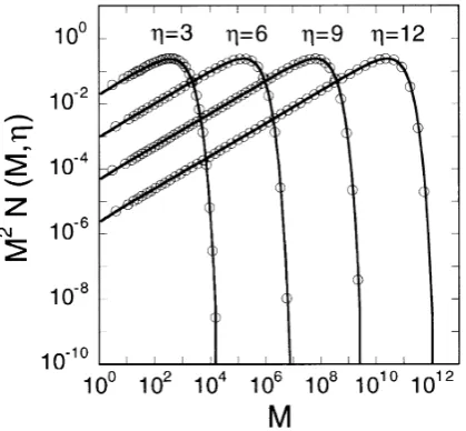
Fig. 1. Comparison between the analytical solution (curves) and the numer-ical solution (circles) for the case ofAi j=i+j. The mass distribution
gives the precise solution of the accumulation process for
Ai j=i+ jas long as the mass of the largest body is much
smaller than the total mass (Tanaka and Nakazawa, 1994). In Fig. 1, we illustrate the mass distribution functions obtained numerically at typical epochs as well as the corresponding analytical solutions. From thisfigure, we can see that the nu-merical simulation can reproduce the analytical solution and find the almost same accuracy of the numerical simulation as that of Wetherill (1990)∗∗.
4.
Comparison between Numerical and Analytical
Solutions for the Case of
A
ij=i
×j
4.1 Method of comparison
In order to check the validity of WS89 method, we perform numerical simulations using our numerical code for the case ofAi j=i×jwhere runaway growth inevitably occurs. The
initial condition is taken as
Nk=Nδ1k, (19)
whereNis the total number of bodies with unit mass. Analyt-ical solution to the stochastic coagulation equation is already presented in Section 2. We also mentioned runaway growth of one body starts atη1 (i.e.,t1/N).
We compare the time evolution of the masses of the largest and the second largest bodies,M1andM2, obtained from the
numerical simulation with those obtained from the solution to the stochastic coagulation equation. In the early stage (i.e., η 1), there exist a large number of bodies in any relevant mass batches and, then, the Smoluchowski equation is still valid (Tanaka and Nakazawa, 1994). Wetherill (1990) showed that their numerical result agrees with the solution to the Smoluchowski equation. Thus, in the early stage, we can use WS89 method as long as we choose appropriately the technical parameters δ and. In runaway growth, as the accumulation process proceeds, the number of runaway bodies becomes a few or one. Generally, because of its sta-tistical property, the Smoluchowski equation cannot describe the subsequent stage where a few bodies grow prominently. Thus, to check validity of WS89 method, we compare the re-sult of WS89 method with the analytic solution to the stochas-tic coagulation equation in the case of Ai j =i × j which is the only case where the solution is known and runaway growth occurs. In order to check whether WS89 method reproduces the solution to the stochastic coagulation equa-tion, the check should be done in the late stage, where the Smoluchowski equation breaks down. Note that the case of
Ai j = i × j has a special property that, for a sufficiently small mass k, the solution nk to the stochastic coagula-tion equacoagula-tion agrees with that to the Smoluchowski equacoagula-tion even in the late stage (Tanaka and Nakazawa, 1994). As runaway growth of one body proceeds, except for the largest one, there exist only sufficient small bodies of which num-bers is well described by the Smoluchowski equation in the case of Ai j =i× j. Then, by subtracting the total mass of the small bodies from the total mass in the system, we also obtain the precise value of the runaway body’s mass from the Smoluchowski equation in this case. In this way, for
∗∗Wetherill (1990) seems to mislabel values of the abscissa in Fig. 4. The values should be from 0 to 13, not from 2 to 15.
Ai j =i ×j, the Smoluchowski equation also can describe
the stage where runaway growth of one body proceeds suf-ficiently, though it cannot describe the stage where runaway growth of one body starts (i.e., aroundη=1). Hence, we make a comparison between the results of WS89 method and the analytic solution to the stochastic coagulation equation especially in the stage where runaway growth of one body starts.
In the comparison, we pay attention to the time develop-ment of the masses of the largest and the second largest bod-ies,M1andM2. For the stage where runaway growth starts,
it is meaningless to compare the numerical result obtained from a single run with the analytical solution because M1
and M2 obtained from the stochastic coagulation equation
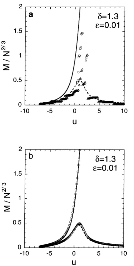
are expectation values. In Fig. 2a, we show the time varia-tion of M1(circles) and M2 (triangles), which are obtained
from a single run, for the case ofN =1×10³,δ=1.3, and =0.01 as a function of the renormalized timeu defined by Eq. (10). In this figure two solutions are quite differ-ent from each other: both M1 and M2 obtained from the
numerical simulation change discontinuously owing to the coalescence with other bodies whereas those obtained from the stochastic coagulation equation change smoothly since they are expectation values. Hence, the analytical solution should be compared with the ensemble mean obtained from a large number of independent runs with different random number generators. The ensemble mean of a body mass at timeη(oru),M, is given by
whereNcis the number of independent runs andMi is the
body mass at timeηobtained by the i-th run. In Fig. 2b, we show the ensemble means ofM1andM2obtained by
per-forming 1000 runs (i.e.,Nc=1000). The ensemble means of
M1andM2 calculated from the numerical simulation agree
with the analytical solutions to the stochastic coagulation equation even in the stage where runaway growth of one body starts. The comparison between the numerical and an-alytical solutions in general view is also shown in Fig. 2c. In both early and late stages, two solutions agree with each other. This means that WS89 method is able to describe pre-cisely the accumulation process if we use suitable parameters
δand.
The technical parametersδ and govern essentially the degree of accuracy of the numerical solutions. If we canfind their values with which the numerical simulation reproduces the analytical solution within a certain level of accuracy and if these values are suitable for actual computational runs in a sense of the needed memory size as well as the elapsed com-puting time, then we can say that WS89 method is valid and useful. Hence, the present aim is tofind a suitable set ofδand
. Tofind appropriate ranges ofδand, we make a compar-ison between two solutions in a quantitative manner. We pay our attention to the followingfive quantities, which charac-terize the time development ofM1andM2(thefive quantities
Fig. 2. The growth of the mass of the largest bodyM1(circles) as well as that of the second largest bodyM2(triangles) for the case ofAi j=i×j
(parameters are put to beδ=1.3,=0.01, andN=1×10³). Panel (a) showsM1andM2obtained by a single run while panels (b) and (c) show those evaluated as the ensemble means of 1000 independent runs. The vertical axis shows the mass normalized byN2/3and abscissa denotes the renormalized timeu. In each panel, expectation values ofM1andM2 evaluated by the analytical solution are also shown by solid and dashed curves, respectively.
average growth speed,M˙1, which is defined by the reciprocal
of the time interval between two epochs,M/N2/3=1 and 2.
Another is the time,η1 (corresponding tou1), at which the
mass of the largest body becomes three times as large as that of the second one;η1is introduced to see in detail the con-nection between masses of the largest and the second largest bodies. As for the growth of the second largest body, we consider three quantities, that is, the mass,M2 max, the time, η2 max(corresponding tou2 max), and the time interval,η2
(corresponding tou2). Here,M2 maxis the maximum mass
of the second largest body (note that, as shown schemati-cally in Fig. 3, the mass of the second largest body initially
Fig. 2. (continued).
Fig. 3. Five quantities which are used for the comparison between the numerical and the analytical solutions in our present study (Note that as the abscissa we useuin place ofηin order to magnify the picture around the stage of beginning of the runaway growth). In thefigure,M˙1 is the average growth speed of the mass of the largest body andu1 is the time when the mass of the largest body,M1, becomes three times as large as that of the second largest body,M2. Furthermore,M2 maxand
u2 maxare the maximum value ofM2and the instant whenM2=M2 max, respectively, andu2is the period, during whichM2≥12M2 max. Note thatη1,η2 max, andη2correspond tou1,u2 max, andu2, respectively, through Eq. (10) or (31).
increases and afterward tends to decrease),η2 maxis the time at which the mass of the second largest body attains the max-imum value, andη2 is the time interval during which it stays with mass greater thanM2 max/2.
Table 1. Relative errors of thefive quantities in typical two cases,δ=1.3 and 3.0. In both cases,Nandare put to be 1000 and 0.01, respectively. δ M˙1 M2 max η2 η1 η2 max
1.3 0.057 −0.066 −0.011 0.0070 −0.022
3.0 0.61 0.0037 −0.33 0.24 0.21
are the quantities obtained from the numerical and analytical solutions, respectively. As a level of accuracy, we demand the following condition:
Xn−Xa
Xa
≤ξ (21)
where
ξ =
0.3, for M˙1,M2 max, andη2,
0.04, for η1andη2 max. (22)
Usually, the relative errors ofη1andη2 maxare small. There-fore, in Eq. (22), we demand a high level of accuracy for these relative errors.
4.2 Validity check of Wetherill and Stewart’s method According to the method of comparison mentioned in the last Subsection, we investigate in detail the validity of WS89 method by simulating the accumulation process for the case ofAi j=i×jwhere runaway growth inevitably occurs in the
course of accumulation. We adoptNc=1000, which will be
justified later in Subsection 4.3. Wefirst show the typical two examples of numerical simulations withN =1000, i.e., the cases of(δ, )=(1.3,0.01)and(3.0,0.01). In the former case, the simulation satisfies the demanded level of accuracy mentioned above and the latter is the case where we cannot obtain precise numerical results. Numerical errors in the two cases are tabulated in Table 1. For the case ofδ =1.3,the errors of all quantities are suppressed sufficiently under the level of accuracy demanded by inequality (21). For the case ofδ =3.0, however, the errors are too large: especially, the relative errors ofη1 andη2 max, are 0.24 and 0.21, respec-tively. Thus, we cannot accept the result of this simulation as a solution though the error ofM2 maxhappens to be small.
For the case of δ = 3, the mass distribution is described by only 6 batches. Hence, it is hard to express the exact accumulation process by such a small number of batches. We see from these two examples that, as a reasonable result, the simulations with smallδ could describe accurately the accumulation process.
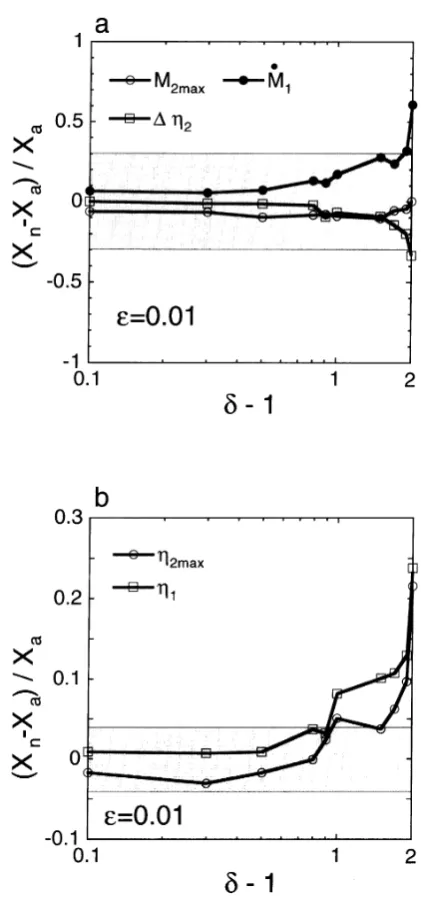
In order to see in detail how the relative errors depend on the adapted value ofδ, we have made 10 simulations with various values ofδ (N andarefixed to be 1000 and 0.01, respectively). As illustrated in Fig. 4a, whenδ is smaller than 2.9, the relative errors of M˙1 andη2 are within the
demanded level. When δ becomes large beyond 2.9, the relative errors increase suddenly and, at the same time, the results of the simulation do not satisfy the condition (21). On the other hand, the errors ofη2 maxandη1are at a low level as long as we are concerned with the case ofδ ≤ 1.5. For
δ ≥ 1.5, they begin to increase almost monotonously and rapidly with an increase inδ(see Fig. 4b). Whenδexceeds
Fig. 4. The behaviors of the relative errors ofM˙1,M2 max,η2(panel (a)), η1, andη2 max(panel (b)) againstδ−1 for the case ofN =1000 ( isfixed to be 0.01). The shaded region denotes the admissible range of errors demanded by condition (21).
1.9, the errors ofη2 maxandη1go out of the admissible range given by the inequality (21). Thus, it is ascertained that, for the case of =0.01, the numerical simulation is valid because it can reproduce approximately the accumulation process (but within the demanded level of accuracy) when
which the simulation fails, is called the critical value ofδ and denoted byδc. For the case of=0.01 andN =1000, we haveδc=1.9. In general, the value ofδcis determined in Fig. 4b instead of Fig. 4a.
The accuracy of the numerical simulation depends not only on the mass division parameterδbut also on the time division parameterwhich determines the time incrementη(see Eq. (16)). As seen from Fig. 4, if we choose a very large value ofδ, the numerical solution departs far from the analytic one even ifis chosen appropriately. The same would be true for: for the value oflarger than a certain critical valuec, the error of the numerical solution is beyond the demanded level of accuracy even ifδis properly chosen. The numerical solution would reproduce accurately the analytical one if both
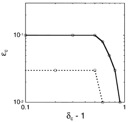
δandare put to be sufficiently small. Hence, there exists a certain curve on theδ−plane such that the error of the numerical solution is suppressed within the demanded level of accuracy as long as a set ofδandis inside the region enclosed by the critical curve (which from now on is called theδc−c curve). In order tofind the δc−ccurve, we have made numerical simulations for the various values of
δ (from 1.1 to 2.0) and (from 0.01 to 1.0). Theδc−c curve obtained from the simulations is shown in Fig. 5 for the case of N = 1000. From Fig. 5, we see that, ifδ is smaller than 1.5, the maximum admissible value of(i.e.,
c) is 0.1 and thatcdecreases suddenly with an increase in
δwhenδ >1.5.
Theδc−ccurve depends on the total number of the system
N. In order to see the dependence of the curve onN, we made two kinds of simulations: one is simulations tofindδcas a function ofNunder thefixed value of(=0.01) and another is those tofindcunder thefixed value ofδ (=1.5). The results of the former and the latter simulations are shown in Figs. 6a and b, respectively. Bothδcandcdecrease with an increase inNand tend to converge to certain values,δc=1.6
Fig. 5. Theδc−ccurve for the case ofN =1000 (solid curve). The numerical simulation withδand, which are chosen from the region enclosed by this curve, could describe the accumulation process within the demanded level of accuracy as long asN≤1×10³. The same curve is also drawn for the limiting case of largeN(dashed line).
Fig. 6. The behaviors ofδc(panel (a)) andc(panel (b)) against the total body number of the systemN. In panels (a) and (b), the other parameters arefixed to be=0.01 andδ=1.5, respectively.
andc=0.03. This convergence means that we canfind an appropriate set ofδandirrespective of the size of the body system if it is large enough. In Fig. 5 we also show the
δc−ccurve in the limit of largeNpresumed from the above results. Though it is difficult to understand quantitatively the behaviors ofcandδcshown in Fig. 6, we say in a qualitative sense that their behaviors are natural: for the case of smallN, a numerical simulation is accomplished with the relatively small number of time steps so that large values ofδandare admitted.
4.3 Sample number for evaluating the ensemble mean
particle growth by the numerical simulation, we take the en-semble mean, performing many runs with different random number generators. We examine here a suitable choice of the number of independent runs for evaluating the ensem-ble mean. For various numbers of the runs (Nc =10, 100,
500, 1000, 2000, and 4000), we have calculated the ensemble means of thefive quantities introduced in Subsection 4.1 and evaluated their relative errors (δandarefixed asδ =1.3 and=0.01). Figure 7 shows the dependence of the rela-tive errors ofM˙1, M2 max, andη2(Fig. 7a) and ofη1 and η2 max(Fig. 7b) as a function of the number of simulationsNc.
From thisfigure, we can see that the relative errors converge if we average the quantities over 100 (or 1000) simulations for the case ofM˙1,M2 max, andη2 (orη1 andη2 max). All
Fig. 7. The dependences of the relative errors ofM˙1,M2 max,η2(panel (a)),η1, andη2 max(panel (b)) on the number of independent simula-tions,Nc. The other parameters are put to beδ= 1.3, = 0.01 and
N=1×10³.
of the numerical results in Subsection 4.2, are evaluated by the ensemble means averaged over 1000 independent runs, which is justified by the above result.
Strictly speaking, the number of samples Nc should be
determined on the basis of the ratio of the dispersion to the mean value. As an example, we consider the averaged value of the mass of the largest body,M1(given by Eq. (20)), and
its standard deviation,M1,s, which is defined by
M1,s=
1
Nc
Nc
i=1 (Mi
1−M1)2. (23)
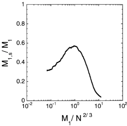
In Fig. 8, we show the ratio of the standard deviation to the averaged value evaluated from 1000 numerical simulations (i.e., Nc = 1000) in whichN,δ, andare put to 1×10⁶,
1.2, and 0.01, respectively. Just before the start of runaway growth (i.e.,M1/N2/3is about 0.1 and the renormalized time
uis about−5 (see also Fig. 2a)),M1,s/M1is relatively small.
But in the vicinity ofM1/N2/3 1 (u 0), the ratio rises
almost to 0.6. Afterwards, the ratio decreases gradually and becomes smaller than 0.1 after M1/N2/3 >7 (u =3). As
conjectured from Fig. 2a, this behavior of M1,s/M1means
that the stochastic property becomes distinct around the stage of the beginning of runaway growth.
From the above results, we can evaluate the number of simulations Nc demanded for obtaining the reliable mean
valueM1(within an accuracy of, say, 3 percent) as
Nc=
1 0.03
M1,s
M1
2
. (24)
Equation (24) yields Nc=400 and 11 whenM1/N2/3=1
and 7, respectively. Therefore, 1000 simulations used in Subsection 4.2 is sufficient. It is worthwhile to note that, as readily conjectured, the behavior ofM1,s/M1shown in Fig. 8
Fig. 8. The ratio of the standard deviation to the expectation value of the mass of the largest body as a function ofM1/N2/3(for the case of
would not be general but depends on the functional form of adoptedAi j. As to this point, we will discuss in Section 5.
5.
The Case of Planetesimal Accumulation
In the previous section, we considered the case where the collisional probability Ai j is proportional to the square of mass, i.e.,Ai j=i×j(note that we say, for example, Ai jis proportional to mass whenAi j =i+ j). In this section, we derive a suitable set ofδandfor describing the planetesimal accumulation process. As readily conjectured, when Ai j
is proportional to a power of mass with a large exponent, runaway growth of one body starts early (Wetherill, 1990) and the mass of the runaway body increases rapidly. In such cases, the numerical simulation becomes hard and strong conditions would be needed for obtaining a precise numerical solution (speaking in our present language,δcandcwould become small). In order to confirm the validity of Wetherill and Stewart’s method for the planetary accumulation process, we examine appropriate ranges ofδandfor the collisional probability in the planetesimal accumulation.
If we neglect the effects of the solar gravity and assume a uniform distribution of planetesimals, we describe the plan-etesimal accumulation process in terms of the surface number density of planetesimals instead of the number density and thenAi jis approximately given by (Makinoet al., 1998)
Ai j= π
the relative velocity between bodies with massesiandj, and
vesc is the escape velocity given by (note that the unit mass is 1)
The scale height of planetesimal swarm with massi,Hi, is proportional to the mean random velocityvi of bodies with
massi. We consider the low velocity case (i.e.,vi j vesc)
where gravitational focusing is effective. It is assumed that the mean random velocities of planetesimals are determined by the energy equipartition between them, i.e.,vi ∝ i−1/2
(Kokubo and Ida, 1996) and that the relative velocityvi j is
determined by the larger mean random velocity as vi j =
max(vi, vj). From the above assumptions, we have forAi j
Ai j =α min(i,j)(i1/3+ j1/3)(i+j), (27)
where α is a certain constant independent of mass. The above collisional probability has the mass dependence as
Ai j ∝ (mass)7/3 if bodies mainly captures the others with
comparable masses to itself, which is satisfied for runaway bodies in this case.
As in the case of Ai j = i × j, we scale the mass and time to describe the stage when runaway growth of one body starts. Makinoet al.(1998) approximately solved the Smolu-chowski equation for the collisional probability given by Eq. (27). Their approximate mass distribution is given by
nk = 2
3N k
−8/3 (28)
for massesksmaller than the high mass end of the distribu-tion. The above mass distribution agrees well with the results of N-body simulation (Kokubo and Ida, 1996) and the sta-tistical simulation (Wetherill and Stewart, 1989, 1993) for the case that collisional fragmentation is not considered. As the accumulation process proceeds, the high mass end of the mass distribution becomes large and the number of plan-etesimals in the high mass end decreases. As a result, the mass ratio of the largest planetesimal to the second largest one increases and runaway growth starts. We consider that runaway growth of one body starts when the largest body be-comes twice massive as the second largest one. Using Eqs. (7) and (28), we roughly evaluate the mass of the largest body at the starting time asM1∼N3/5. The starting time is
also evaluated asη=N t 0.2α−1from the Smoluchowski equation. Using Eq. (15), we obtain the growth rate of the largest body as
As readily seen from the above estimation, it is convenient to introduce the following scaled massM˜ and timeu:
˜
M =M/N3/5, (30)
u =N2/5(αη−0.2). (31)
If we useM˜ andu, the scaled growth rate of the largest body,
dM˜/du, does not depend on the total mass N andα. That is, the growth curve of the largest and second largest bodies in theu−M/N3/5plane is almost independent ofN.
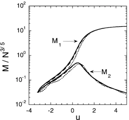
In Fig. 9, we show the growth curves of the runaway bodies which are obtained from numerical simulations with various
δ (δ =1.2, 1.5, and 2.0) and =0.01 (N being put to be
Fig. 9. The growth of the largest and the second largest bodies numerically found for the case ofAi j=α×min(i,j)(i1/3+j1/3)(i+j). The vertical
axis shows the mass normalized byN3/5. The masses are obtained by ensemble means of 1000 runs and the abscissa is the renormalized time,
1000). The simulations withδ=1.2 and 1.5 give almost the same growth curves of the largest and the second largest bod-ies. Hence we presume the precise solution to the stochastic coagulation equation. For the case ofδ=2, the starting time of runaway growth of one body delays compared with that of the simulation withδ =1.2: the time at which the mass of the largest body becomesN3/5and the time at which the
sec-ond largest body experiences its maximum mass are shifted toward positiveu by a factor of 0.5. In the previous case (where Ai j=i×j), we frequently observed the time delay due to largeδand, hence, such a feature would be general.
Now, we make a quantitative comparison by the same way as Section 4. Instead of Xa calculated from the analytical
solution, we use the values Xcwhich is obtained from the
simulation withδ=1.1 and=0.01. Since we know that the simulations withδsmaller than 1.5 give the almost same solutions and that the simulation with smallδ can describe the accumulation process precisely, it would be proper to replaceXabyXc. Demanding the level of accuracy given by
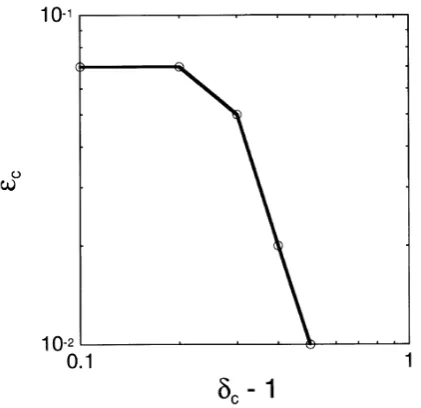
inequality (21) and Eq. (22), we obtain theδc−ccurve for the case ofN =1000 which is shown in Fig. 10. Theδc−ccurve behaves similarly with that of the case ofAi j =i×j(Fig. 5), though the values ofδcandcbecome small: especially, the value ofcbecomes very small (c =0.07) compared with the previous case even whenδis as small as 1.1 or 1.2 and, furthermore, decreases suddenly with an increase inδwhen
δ >1.3.
In Fig. 11, we illustrate howδcdepends on the total mass of the body systemN(beingfixed to be 0.01) as well as for the case ofc(δisfixed to be 1.2). As seen from thefigures,
δcandcdecrease with an increase inNand converge to 1.3 and 0.04, respectively, in the limit of largeN. The behaviors ofδcandcare observed similarly to the case ofAi j=i×j.
However, compared with the limiting values ofδcandcfor the case ofAi j=i×j(δc=1.6 andc=0.03),δcis rather small in this case althoughcis almost the same. This is due to the fact thatAi jdepends strongly on the mass in this case.
Fig. 10. The same as Fig. 5, but for the case of Ai j = α ×
min(i,j)(i1/3+j1/3)(i+j).
Fig. 11. The same as Fig. 6, but for the case of Ai j = α×
min(i,j)(i1/3+j1/3)(i+j).
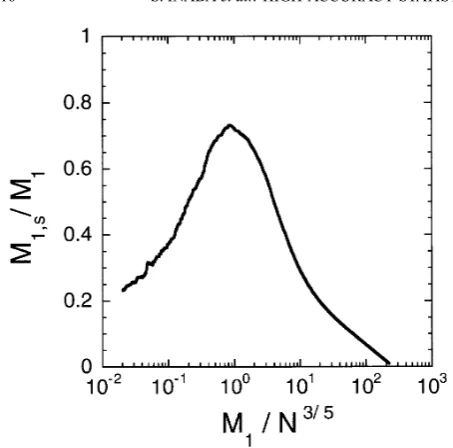
Fig. 12. The same as Fig. 8, but for the case of Ai j = α ×
min(i,j)(i1/3+j1/3)(i+j).
The ratio of the standard deviationM1,s(given by Eq. (23))
to the mean valueM1(given by Eq. (20)) of the mass of the
largest body is illustrated in Fig. 12 as a function ofM1/N3/5.
In a qualitative sense thisfigure is quite similar to Fig. 8: the ratio has a maximum value in the vicinity of M1/N3/5 =1 which corresponds tou = 0 and decreases toward the di-rection of large|u|. However, the peak value ofM1,s/M1is
as large as 0.75 in this case (in the case ofAi j =i× j the
peak value is about 0.6). As mentioned in the Subsection 4.3,M1,s/M1becomes large whenAi jis given by the power
law of the mass with a high exponent. Thus, in the numerical simulation of the planetary accumulation by the use of WS89 method we must take the ensemble mean over about 500 in-dependent simulations if we are interested, especially, in the planetary growth around the stage of beginning of runaway growth.
6.
Conclusion and Discussion
In the present study we checked the validity and usefulness of the numerical method, proposed by Wetherill and Stewart (1989), for describing the late stage of planetary accumula-tion by comparing the numerical soluaccumula-tion of WS89 method (or more exactly, the ensemble mean of a sufficiently large number of simulations) with the analytical solution (or the well-evaluated numerical solution). As mentioned in Sec-tion 3, our numerical code, which was reconstructed on the basis of WS89 method, is optimized by the two technical parametersδand: δis the ratio of the masses of adjacent mass batches and is the parameter determining the time interval in the numerical time integration.
We considered the two cases, Ai j = i × j and α× min(i,j)(i1/3+ j1/3)(i + j), as for the collisional
proba-bility. The latter case corresponds to the simplified model of the planetesimal accumulation. In the former case the analytic solutions to the stochastic coagulation equation is known while in the latter case no analytic solution is found
yet. In both cases runaway growth starts at a certain time. By the comparison between numerical and analytical so-lutions for the case ofAi j =i×j, we confirmed that the
en-semble mean obtained from WS89 method reproduces well the analytical solution when both δ and are sufficiently small. Furthermore, we found that the numerical simulation can describe the accumulation process within an admissible level of accuracy when the values ofδandare smaller than certain critical values (which are denoted byδc andc, re-spectively). The critical valuesδcandcare given by 1.6 and 0.03, respectively when the initial number of particlesN, is large enough.
We examined the critical values δc andc, in the sim-plified case of planetesimal accumulation (i.e., Ai j = α×
min(i,j)(i1/3+ j1/3)(i +j)). Since no analytical solution
exist in this case, we adopted a numerical solution with suffi -ciently smallδandas a standard measure. Then, the critical values were obtained asδc =1.3 andc=0.04, irrelevant of the initial number of particles. Compared with the case of Ai j =i×j,δcis somewhat small whilecis almost the same. This would be due to strong dependence of Ai j on mass (Ai j∝(mass)7/3).
Since WS89 method contains the stochastic procedures, we examined how large the dispersion of the results is and how many runs are needed for obtaining a reliable ensem-ble mean. From the ratio of the standard deviation to the expectation value, which are obtained by the numerical sim-ulations, we found that the demanded number of runs is as large as 400 (or 500) for the case of Ai j =i × j (or Ai j =
α×min(i,j)(i1/3+j1/3)(i+j)) around the time when
run-away growth starts. But, before that, the demanded number of runs is rather small (10 or so).
In real planetary accumulation, the dependence of the col-lisional probabilityAi jon masses of colliding particles would
be weaker than that we adopted (Ai j ∝ (mass)7/3).
Gen-erally, δc andc become larger when Ai j depends weakly on the mass. Hence, we reach the following conclusions: WS89 method can describe the planetary accumulation pro-cess within a reasonable level of accuracy if we adopt the values ofδandsmaller than 1.3 and 0.03, respectively, and if we evaluate the ensemble mean on the basis of 500 nu-merical simulations. Because Wetherill and Stewart (1989) and (1993) used the value ofδsmaller than 1.1 and 1.2, re-spectively, they used their method correctly and, thus, give reliable results. On the other hand, since they did not perform sufficient averaging over an ensemble of similar accumula-tion process, divergence from the mean value for the growth of the largest body might be found. From the viewpoint of the numerical handling, the values of δ (= 1.3) is not so small comparing with those in other numerical simulations. In fact, when δ = 1.3, we can cover the mass coordinate over 1×10²⁰mass range only with 180 mass batches. Thus,
it is concluded that the new method proposed by Wetherill and Stewart is the valid and useful method for pursuing the planetary accumulation process.
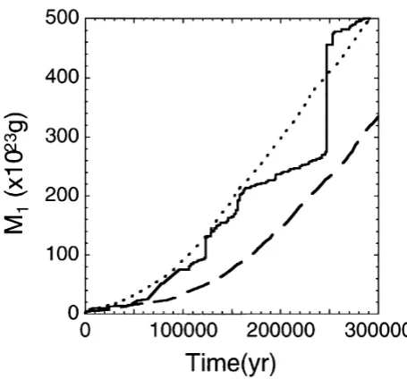
simultane-Fig. 13. The preliminary result of comparison between the statistical sim-ulation andN-body simulation (solid curve). The dotted and dashed curves indicate the evolution of the largest body’s mass calculated by WS89 method withδ=1.1 and 2.5, respectively.
ously. In the subsequent paper, we will complete our statis-tical code which simulate the accumulation process coupled with the velocity evolution and examine the accuracy of our statistical code, by comparing the results of the statistical code with those of N-body direct simulations. In Fig. 13, we show a preliminary comparison of our statistical code withN-body simulation by Kokubo and Ida (1998). As to the time evolution of the random velocity (i.e., eccentricities and inclinations), we adopted the formulation by Stewart and Ida (1998). The results of Greenzweig and Lissauer (1992) is used for the collisional probability between planetesimals. Initially the masses of all bodies are 1×10²³g and the total number of bodies is 3000. The dotted and dashed curves in-dicate the evolution of the largest body’s mass calculated by the statistical code withδ=1.1 and 2.5, respectively, and the solid curve gives the result ofN-body simulation. The mass of the largest body obtained by our statistical code changes smoothly since we take the ensemble mean and, while,N -body simulation gives the discontinuous growth because it is a single calculation. Except for the statisticalfluctuations in theN-body simulation, our statistical code well reproduces the results of theN-body simulation in the case ofδ =1.1. On the other hand, in our statistical simulation withδ=2.5, the growth of the largest body delays as shown in the previ-ous cases. Therefore, even if we consider the accumulation process coupled with the velocity evolution, the criterion de-rived in this paper is available. The detail of our statistical code and the comparison with N-body simulations will be described in the subsequent paper.
Acknowledgments. The authors are indebted to S. Ida and H. Emori for valuable comments. We express our gratitude to E. Kokubo for giving us the data of N-body simulation. We also thank R. Nakamura for introducing the literature on the stochastic
coagulation equation in thefield of atmospheric sciences. We are grateful to S. Watanabe and G. Stewart for careful reviews of the paper. This work has been supported in part by Grand-in-Aid for General Scientific Research (B) (No. 09440089). The computation has been made by Cray C916 at the Computer Center of Tokyo Institute of Technology.
References
Aarseth, S. J., D. N. C. Lin, and P. L. Palmer, Evolution of planetesimals. II. Numerical simulations,Astrophys. J.,403, 351–376, 1993. Barge, P. and R. Pellat, Mass spectrum and velocity dispersions during
planetesimal accumulation. I. Accretion,Icarus,93, 270–287, 1991. Bayewitz, M. H., J. Yerushalmi, S. Katz, and R. Shinnar, The extent of
correlations in a stochastic coalescence process,J. Atmos. Sci.,31, 1604– 1614, 1974.
Beaug´e, C. and S. J. Aarseth, N-body simulation of planetary formation,
Mon. Not. R. Astron. Soc.,245, 30–39, 1990.
Greenberg, R., J. Wacker, C. R. Chapman, and W. K. Hartmann, Planetes-imals to planets: Numerical simulation of collisional evolution,Icarus, 35, 1–26, 1978.
Greenzweig, Y. and J. J. Lissauer, Accretion rates of protoplanets II. Gaus-sian distributions of planetesimal velocities,Icarus,100, 440–463, 1992. Hayashi, C., K. Nakazawa, and Y. Nakagawa, Formation of the solar system, inProtostars and Planets II, edited by D. C. Black and M. S. Matthews, 1100 pp., Univ. of Arizona Press, Tucson, 1985.
Kokubo, E. and S. Ida, On runaway growth of planetesimals,Icarus,123, 180–191, 1996.
Kokubo, E. and S. Ida, Formation of protoplanets from planetesimals in the solar nebula,Icarus, 1998 (submitted).
Lecar, M. and S. J. Aarseth, A numerical simulation of the formation of the terrestrial planets,Astrophys. J.,305, 564–579, 1986.
Lushnikov, A. A., Coagulation infinite systems,J. Colloid Interface Sci., 65, 276–285, 1978.
Makino, J., T. Fukushige, Y. Funato, and E. Kokubo, On the mass distri-bution of planetesimals in the early runaway stage,New Astronomy,3, 411–416, 1998.
Marcus, A. H., Stochastic coalescence,Technometrics,10, 133–143, 1968. Nakagawa, Y., C. Hayashi, and K. Nakazawa, Accumulation of
planetesi-mals in the solar nebula,Icarus,54, 361–376, 1983.
Ohtsuki, K., Y. Nakagawa, and K. Nakazawa, Growth of the earth in nebula gas,Icarus,75, 552–565, 1988.
Safronov, V. S.,Evolution of the Protoplanetary Cloud and Formation of the Earth and Planets, Nauka, Moscow, 1969 (Transl. 1972 NASA TT F-677).
Smoluchowski, M. V., Drei vortrage uber diffusion, brownshe molekularbe-wegung und koagulation von kolloidteilchen,Phys. Zeits.,17, 557–571; 585–599, 1916.
Spaute, D., S. J. Weidenschilling, D. R. Davis, and F. Marzari, Accretional evolution of a planetesimal swarm: 1. A new simulation,Icarus,92, 147–164, 1991.
Stewart, G. R. and S. Ida, Velocity evolution of planetesimals: Unified analytical formulae and comparison with N-body simulations,Icarus, 1998 (submitted).
Tanaka, H. and K. Nakazawa, Stochastic coagulation equation and validity of the statistical coagulation equation,J. Geomag. Geoelectr.,45, 361– 381, 1993.
Tanaka, H. and K. Nakazawa, Validity of the statistical coagulation equation and runaway growth of protoplanets,Icarus,107, 404–412, 1994. Trubnikov, B. A., Solution of the coagulation equations in the case of bilinear
coefficient of adhesion of particles,Sov. Phys. Dokl.,16, 124–126, 1971. Wetherill, G. W., Comparison of analytical and physical modeling of
plan-etesimal accumulation,Icarus,88, 336–354, 1990.
Wetherill, G. W. and G. R. Stewart, Accumulation of a swarm of small planetesimals,Icarus,77, 330–357, 1989.
Wetherill, G. W. and G. R. Stewart, Formation of planetary embryos: Ef-fects of fragmentation, low relative velocity, and independent variation of eccentricity and inclination,Icarus,106, 190–209, 1993.