1
Dynamic Asset Allocation in a
Conditional Value-at-risk
Framework
Lin Zhi Tan
Submitted by Lin Zhi Tan to the University of Exeter as a thesis for the degree of Doctor of Philosophy in Finance In May 2013
This thesis is available for Library use on the understanding that it is copyright material and that no quotation from the thesis may be published without proper acknowledgement.
I certify that all material in this thesis which is not my own work has been identified and that no material has previously been submitted and approved for the award of a degree by this or any other University.
2 Acknowledgements
My deepest gratitude goes first and foremost to Professor Richard Harris, my supervisor, for his encouragement and continuous support of my PhD research. He has guided me through all the stages of research and writing of this thesis. Without his consistent and illuminating instruction, this thesis could not have reached its present form. I am very lucky to have such an excellent supervisor and mentor for my PhD study.
I would like to acknowledge the Board of Examiners for their constructive comments and suggestions in my viva.
I would also like to express my gratitude to Dr. Jian Shen for her help with data and useful comments.
I am grateful to the staff at the University of Exeter Business School, the IT officers and the librarians for their help to support my research.
I gratefully acknowledge the financial support from the Business School of the University of Exeter to make me realise the doctoral dream.
This thesis is dedicated to my families. I would like to take this opportunity to say thank you to my beloved families for their loving consideration and encouragement through all these years. Without your support and encouragement, I could not afford to come to the UK and finish my PhD and master’s degree in Exeter.
I would like to say thanks to my friends. I really enjoyed my time in Exeter with your company.
3 Abstract
The thesis first extends the original Black-Litterman model to dynamic asset allocation area by using the expected conditional equilibrium return and conditional covariances based on three volatility models (the DCC model, the EWMA model and the RW model) into the reverse optimisation of the utility function (the implied BL portfolio) and the maximised Sharpe ratio optimisation model (the SR-BL portfolio). The momentum portfolios are inputted as the view portfolios in the Black-Litterman model. The thesis compares performance of the dynamic implied BL portfolio and the dynamic SR-BL portfolio in the single period and multiple periods with in-sample analysis and out-of-sample analysis. The research finds that dynamic BL portfolios can beat benchmark in in-sample and out-of-sample analysis, the dynamic implied BL portfolio always show better performance than the dynamic SR-BL portfolio. The empirical VaR and CVaR of the dynamic SR-BL portfolios are much higher than that of the dynamic implied BL portfolio. The dynamic BL portfolios based on the DCC volatility model perform best in contrast to other two volatility models.
In the aim of improving performance of SR-BL portfolios, the thesis further constructs dynamic BL portfolios based on two new optimisation models including maximised reward to VaR ratio optimisation model (MVaR-BL portfolios) and maximised reward to CVaR ratio optimisation model (MCVaR-BL portfolios) with assumption of the normal distribution and the t-distribution at confidence levels of 99%, 95% and 90%. The thesis compares performance of the dynamic MVaR-BL portfolio and the dynamic MCVaR-BL portfolio in the single period and multiple periods with in-sample analysis and out-of-sample analysis. There are three main findings. Firstly, both the MVaR-BL portfolio and the MCVaR-BL portfolio could improve the dynamic SR-BL portfolio performance at moderate confidence levels. Secondly, the MVaR-BL portfolio and the MCVaR-BL portfolio show similar performance with normal distribution assumption, the MCVaR-BL portfolio performs better than the MVaR-BL with t-distribution assumption at certain confidence levels in single period and multiple periods. Thirdly, the performance of the DCC-BL portfolio with t-distribution assumption is superior to the performance of the DCC-BL portfolio with normal distribution assumption.
4
As the result of higher empirical VaR and CVaR of dynamic SR-BL portfolios, the thesis develops to constrain VaR and CVaR in construction of dynamic BL portfolios with assumption of the normal distribution and the t-distribution at confidence levels of 99%, 95% and 90%. The research studies the effect of assumptions of two distributions, three confidence levels and levels of the VaR constraint and the CVaR constraint on dynamic BL portfolios. Both in-sample performance and out-of-sample performance could be improved by imposing constraints, and they suggest adding moderate CVaR constraints to maximal Sharpe ratio optimisation model with t-distribution at certain confidence level could obtain the best dynamic DCC-BL portfolio performance in the single period and multiple periods. The performance evaluation criterion (higher Sharpe ratio, reward to VaR ratio, and reward to CVaR ratio) would affect the choice of optimisation models in dynamic asset allocation.
5 List of Contents Acknowledgements ... 2 Abstract ... 3 List of Contents ... 5 List of Tables ... 10 List of Figures ... 14 List of Appendices ... 15 List of Abbreviations ... 17 CHAPTER 1 INTRODUCTION ... 18
1.1 Background and Rationale ... 18
1.2 Research Aims and Questions ... 22
1.3 The Contributions of this Thesis ... 23
1.4 Structure of the Thesis ... 26
CHAPTER 2 ASSET ALLOCATION FRAMEWORK AND RISK MEASURES 28 2.1 Mean-Variance Analysis and Modern Portfolio Theory ... 28
2.1.1 Classical Mean-Variance Framework ... 28
2.1.1.1 Assumptions ... 28
2.1.1.2 Mathematical Model... 29
2.1.1.3 Efficient Frontier ... 31
2.1.2 Mean-Variance Analysis with Risk-Free Asset and Capital Asset Pricing Model ... 32
2.1.3 Criticisms of the Mean-Variance Approach ... 34
2.1.4 Extension of the Traditional Mean-Variance Approach ... 37
2.2 Risk Measures ... 39
2.2.1 Value-at-Risk ... 40
2.2.2 Conditional Value-at-Risk ... 42
2.3 Conclusions ... 44
CHAPTER 3 LITERATURE REVIEW OF THE BLACK-LITTERMAN MODEL 49 3.1 Introduction ... 49
3.2 The Black-Litterman Model ... 50
3.2.1 The Implied Equilibrium Return ... 52
3.2.2 Investor Views ... 54
3.2.3 Combination of Both Perspectives ... 57
3.2.4 Unconstrained Optimal Portfolio ... 58
3.3 Extensions of the Black-Litterman Model ... 60
3.3.1 Incorporating Momentum Trading Strategies into the Black-Litterman Model ... 64
3.3.2 Alternative Risk Measures in the Black-Litterman Approach ... 65
3.3.3 A VaR Black-Litterman Model for the Construction of Absolute Return Fund-of-funds ... 67
6
3.4 Conclusions ... 69
CHAPTER 4 DATA AND METHODOLOGY ... 70
4.1 Data ... 71
4.2 Methodology ... 73
4.2.1 Estimation of Time-Varying Covariance ... 73
4.2.1.1 Covariance Matrix via Historical Rolling Window Estimators ... 73
4.2.1.2 Covariance Matrix via Exponential Weighted Estimators... 74
4.2.1.3 Covariance Matrix via Dynamic Conditional Correlation Model .. 75
4.2.2 Dynamic BL Model ... 76
4.2.2.1 Conditional Equilibrium Return ... 77
4.2.2.2 Incorporating Momentum Strategies to Generate Views ... 78
4.2.2.3 Combining Conditional Equilibrium Returns and Views Together ... 78
4.2.3 Unconstrained Dynamic BL Portfolio ... 79
4.2.4 VaR-Constrained Dynamic BL Portfolio ... 81
4.2.5 CVaR-Constrained Dynamic BL Portfolio ... 82
4.2.6 BL Portfolio’s Performance Analysis ... 82
4.2.6.1 Single Period Optimisation Statistics ... 84
4.2.6.2 Performance Evaluation ... 84
4.3 Conclusions ... 86
CHAPTER 5 IN-SAMPLE DYNAMIC BLACK-LITTERMAN PORTFOLIOS ... 90
5.1 Construction of the Unconstrained Black-Litterman Portfolio ... 92
5.1.1 Benchmark Portfolio ... 92
5.1.2 Time-Varying Variance and Covariance Matrix ... 93
5.1.3 The Risk Aversion Coefficient ... 94
5.1.4 The Implied Equilibrium Return ... 95
5.1.5 Inputting Views with the Momentum Strategy ... 96
5.1.6 Black-Litterman Expected Return and Covariance Matrix ... 98
5.1.7 Comparison of Unconstrained Portfolio Optimisation Models ... 99
5.1.7.1 Unconstrained Black-Litterman Portfolio Frontier ... 99
5.1.7.2 Unconstrained Black-Litterman Portfolio Optimisation Statistics ... 100
5.1.8 Unconstrained Black-Litterman Portfolio ... 101
5.1.8.1 Construction of the Implied Black-Litterman Portfolio and the Sharpe Ratio Black-Litterman Portfolio ... 101
5.1.8.2 Construction of the MVaR-BL Portfolio ... 104
5.1.8.3 Effect of Distribution Assumption and Confidence Levels on DCC-MVaR-BL Portfolio ... 107
5.1.8.4 Construction of the MCVaR-BL Portfolio ... 108
5.1.8.5 Effect of Distribution Assumption and Confidence Levels on DCC-MCVaR-BL Portfolio ... 110
7
5.1.9 Performance Evaluation of the Unconstrained BL Portfolios ... 111
5.1.9.1 Single Period Performance ... 111
5.1.9.2 Multiple Periods Performance ... 114
5.1.10 Conclusions ... 117
5.2 Value-at-Risk-Constrained Black-Litterman Portfolio ... 119
5.2.1 Construction of the VaR-Constrained BL Portfolio ... 119
5.2.1.1 VaR-Constrained BL Portfolio Frontier ... 119
5.2.1.2 Weights of VaR-Constrained BL Portfolios ... 120
5.2.2 Performance Evaluation ... 122
5.2.2.1 Single Period Performance ... 122
5.2.2.2 Multiple Periods Performance ... 123
5.2.3 Effects of VaR Constraints, Distributions and Confidence Levels .. 125
5.2.3.1 Effects on Optimisation Model ... 125
5.2.3.2 Effects on Weights Solutions ... 125
5.2.3.3 Effects on Portfolio Performance in the Single Period ... 126
5.2.3.4 Effects on Portfolio Performance in Multiple Periods ... 127
5.2.4 Conclusions ... 130
5.3 Conditional Value-at-Risk-Constrained Black-Litterman Portfolio . 131 5.3.1 Construction of the CVaR-Constrained BL Portfolio ... 132
5.3.1.1 CVaR-Constrained BL Portfolio Frontier ... 132
5.3.1.2 Weights of CVaR-Constrained BL Portfolios ... 133
5.3.2 Performance Evaluation ... 135
5.3.2.1 Single Period Performance ... 135
5.3.2.2 Multiple Periods Performance ... 137
5.3.3 Effects of CVaR Constraints, Distributions and Confidence Levels 138 5.3.3.1 Effects on Optimisation Model ... 138
5.3.3.2 Effects on Weight Solutions ... 139
5.3.3.2 Effects on Portfolio Performance in the Single Period ... 140
5.3.3.3 Effects on Portfolio Performance in Multiple Periods ... 142
5.3.4 Conclusions ... 144
CHAPTER 6 OUT-OF-SAMPLE DYNAMIC BLACK-LITTERMAN PORTFOLIOS ... 221
6.1 Out-of-sample Dynamic Unconstrained BL Portfolios ... 221
6.1.1 Construction of Out-of-Sample Unconstrained BL Portfolio ... 222
6.1.1.1 Estimation of Implied Equilibrium Return ... 222
6.1.1.2 Estimation of Views Portfolio ... 223
6.1.1.3 Estimation of BL Expected Return in out of sample ... 224
6.1.1.4 Construction of Out-of-Sample Implied BL Portfolios and SR-BL Portfolios ... 224
6.1.1.5 Construction of the Out-of-Sample Unconstrained MVaR-BL Portfolios ... 226
6.1.1.6 Construction of Out-of-Sample MCVaR-BL Portfolios ... 229
8
6.1.2.1Out-of-sample Implied BL portfolio and SR-BL portfolio ... 232
6.1.2.2 Out-of-sample MVaR-BL portfolio ... 232
6.1.2.3 Out-of-sample MCVaR-BL portfolio ... 233
6.1.3 Multiple Period Out-of-Sample Performance ... 235
6.1.3.1 Out-of-sample Implied BL portfolio and SR-BL portfolio ... 235
6.1.3.2 Out-of-sample MVaR-BL portfolio ... 236
6.1.3.3 Out-of-sample MCVaR-BL portfolio ... 236
6.1.4 Conclusions ... 237
6.2 Out-of-sample Dynamic VaR-Constrained BL Portfolios ... 239
6.2.1 Construction of VaR-Constrained BL Portfolios ... 239
6.2.2 Single Period Out-of-Sample VaR-Constrained BL Performance .. 240
6.2.3 Multiple Periods Out-of-Sample VaR-Constrained BL Performance ... 241
6.2.4 Effects of Distributions and Confidence Levels ... 242
6.2.4.1 Effects on Weights of the Out-of-sample VaR-Constrained BL Portfolio ... 242
6.2.4.2 Effects on the Out-of-sample VaR-Constrained BL Portfolios Performance in the Single Period ... 243
6.2.4.3 Effects on the Out-of-sample VaR-Constrained BL Portfolios Performance in Multiple Periods ... 243
6.2.4 Conclusions ... 245
6.3 Out-of-sample Dynamic CVaR-Constrained BL Portfolios ... 246
6.3.1 Construction of Out-of-sample CVaR-Constrained BL Portfolios ... 246
6.3.2 Single Period Out-of-Sample CVaR-Constrained BL Portfolio Performance ... 248
6.3.3 Multiple Period Out-of-Sample Performance CVaR-Constrained BL Portfolio Performance... 248
6.3.4 Effects on Out-of-sample CVaR-Constrained BL Portfolios Performance ... 250
6.3.4.1 Effects on Weights of the Out-of-sample CVaR-Constrained BL Portfolio ... 250
6.3.4.2 Effects on the out-of-sample CVaR-Constrained BL portfolios performance in the single period ... 251
6.3.4.3 Effects on the out-of-sample CVaR-Constrained BL portfolios performance in multiple periods ... 252
6.3.5 Conclusions ... 254
6.4 Out-of-sample Risk-Adjusted BL Portfolio ... 255
6.4.1 Construction of the Risk-Adjusted BL Portfolio ... 255
6.4.1.1 Estimation of Risk-Adjusted Implied Equilibrium Return ... 255
6.4.1.2 Estimation of Risk-Adjusted BL Expected Return ... 257
6.4.1.3 Construction of Unconstrained Risk-Adjusted BL Portfolios ... 257
6.4.2 Single Period Out-of-Sample Risk-Adjusted BL Portfolio Performance ... 259
9
6.4.3 Multiple-Period Out-of-Sample Risk-Adjusted BL Portfolio
Performance ... 260 6.4.4 Conclusions ... 262 CHAPTER 7 CONCLUSIONS ... 316 7.1 Conclusions ... 316 7.2 Limitations ... 320 7.3 Future Research ... 321 REFERENCES ... 323
10 List of Tables
Table 4.1 Summary Statistics for the FTSE Sector Indices Excess Returns Table 4.2 Time Series Property
Table 5.1.1 Benchmark Portfolio Performance and Tail Risk
Table 5.1.2 Risk Aversion Coefficient and Implied Equilibrium Return in August 1998
Table 5.1.3 The Views Portfolio Weights, Expected Return and Confidence Variance in August 1998
Table 5.1.4 The Views Portfolio Weights, Expected Return and Confidence Variance in November 1998
Table 5.1.5 Portfolio Performance of the Momentum Portfolio and Benchmark Portfolio
Table 5.1.6 The BL Expected Returns for Each Index in August 1998 Table 5.1.7 The BL Expected Returns for Each Index in November 1998 Table 5.1.8 Statistics for Unconstrained BL Portfolio Optimisation in August 1998
Table 5.1.9 Weights in the Unconstrained Implied BL Portfolio and the SR-BL Portfolio in August 1998
Table 5.1.10 Weights in the Unconstrained Implied BL Portfolio and the SR-BL Portfolio in November 1998
Table 5.1.11 Weights in the Unconstrained MVaR-BL Portfolio in August 1998 Table 5.1.12 Weights in the Unconstrained MVaR-BL Portfolio in November 1998
Table 5.1.13 Effect of Distribution Assumptions and Confidence Levels on MVaR-BL Portfolio Weights
Table 5.1.14 Weights in the Unconstrained MCVaR-BL Portfolio in August 1998 Table 5.1.15 Weights in the Unconstrained MCVaR-BL Portfolio in November 1998
Table 5.1.16 Effect of Distribution Assumptions and Confidence Levels on MCVaR-BL Portfolio Weights
Table 5.1.17 Single Period Unconstrained BL Portfolio Performance Evaluation Table 5.1.18 Unconstrained BL Portfolio Performance in Multiple Periods (Nov 94 – May 10)
11
Table 5.1.19 Unconstrained BL Portfolio Performance in a Sub-period (Aug 98 – May 10)
Table 5.2.1 Weights in the VaR-Constrained BL Portfolio in August 1998 Table 5.2.2 Weights in the VaR-Constrained BL Portfolio in November 1998 Table 5.2.3 VaR-Constrained BL Portfolio Performance in the Single Period Table 5.2.4 VaR-Constrained BL Portfolio Performance in Multiple Periods Table 5.2.5 Effects on the VaR-Constrained BL Portfolio Optimisation (Aug 1998)
Table 5.2.6 Effects on Weights of Out-of-Sample VaR-Constrained BL Portfolio (Aug 98)
Table 5.2.7 Effects on VaR-Constrained SR-BL Portfolio Performance Evaluation (Aug 98)
Table 5.2.8 Effects on VaR-Constrained SR-BL Portfolio Performance Evaluation (Nov 98)
Table 5.2.9 Effects on VaR-Constrained BL Portfolio Performance in Multiple Periods (Nov 94-May 10)
Table 5.2.10 Effects on VaR-Constrained BL Portfolio Performance in Sub-period (Aug 98-May 10)
Table 5.3.1 Weights in the CVaR-Constrained BL Portfolio in August 1998 Table 5.3.2 Weights in the CVaR-Constrained BL Portfolio in November 1998 Table 5.3.3 CVaR-Constrained BL Portfolio Performance in the Single Period Table 5.3.4 CVaR-Constrained BL Portfolio Performance in Multiple Periods Table 5.3.5 Effects on CVaR-Constrained BL Portfolio Optimisation (Aug 98) Table 5.3.6 Effects on Weights of the CVaR-Constrained BL Portfolio (Aug 98) Table 5.3.7 Effects on CVaR-Constrained SR-BL Portfolio Performance
Evaluation (Aug 98)
Table 5.3.8 Effects on CVaR-Constrained SR-BL Portfolio Performance Evaluation (Nov 98)
Table 5.3.9 Effects on CVaR-Constrained BL Portfolio Performance in Multiple Periods (Nov 94-May 10)
Table 5.3.10 Effects on CVaR-Constrained BL Portfolio Performance in Sub-period (Aug 98-May 10)
Table 6.1.1 Out-of-sample Risk Aversion Coefficient and Implied Equilibrium Return in September 2003
12
Table 6.1.2 Out-of-Sample Views Portfolio Weights, Expected Return and Confidence Variance in September 2003
Table 6.1.3 Out-of-sample Portfolio Performance of the Momentum Portfolio and Benchmark Portfolio
Table 6.1.4 The Out-of-sample BL Expected Returns for Each Index in September 2003
Table 6.1.5 Weights in the Out-of-sample Unconstrained Implied BL Portfolio and a SR-BL Portfolio in September 2003
Table 6.1.6 Weights in the Out-of-sample Unconstrained MVaR-BL portfolio in September 2003
Table 6.1.7 Effect of Distribution Assumptions and Confidence Levels on out-of-sample MVaR-BL Portfolio Weights
Table 6.1.8 Weights in the Out-of-sample Unconstrained MCVaR-BL portfolio in September 2003
Table 6.1.9 Effect of Distribution Assumptions and Confidence Levels on out-of-sample MCVaR-BL Portfolio Weights
Table 6.1.10 Out-of-Sample Unconstrained BL Portfolios Performance Evaluation in Single Period
Table 6.1.11 Out-of-sample Unconstrained BL Portfolio Performance in Multiple Periods (Sep 03 – May 10)
Table 6.2.1 Weights in the Out-of-sample VaR-Constrained BL Portfolio in September 2003
Table 6.2.2 Out-of-sample VaR-Constrained BL Portfolio Performance in the Single Period
Table 6.2.3 Out-of-sample VaR-Constrained BL portfolio Performance in Multiple Periods
Table 6.2.4 Effects on Weights of VaR-Constrained BL Portfolio (Sep 03)
Table 6.2.5 Effects on out-of-sample VaR-constrained BL Portfolio Performance Evaluation (Sep 03)
Table 6.2.6 Effects on out-of-sample VaR-Constrained BL Portfolio Performance in Multiple Periods (Sep 03-May 10)
Table 6.3.1 Weights in the Out-of-sample CVaR-Constrained BL Portfolio in September 2003
Table 6.3.2 Out-of-sample CVaR-Constrained BL Portfolio Performance in the Single Period
13
Table 6.3.3 Out-of-sample CVaR-Constrained BL Portfolio Performance in Multiple Periods
Table 6.3.4 Effects on Weights of CVaR-Constrained BL Portfolio (Sep 03) Table 6.3.5 Effects on Out-of-sample CVaR-Constrained SR-BL Portfolio Performance Evaluation (Sep 03)
Table 6.3.6 Effects on Out-of-sample CVaR-Constrained BL Portfolio Performance in Multiple Periods (September 03-May 10)
Table 6.4.1 Out-of-sample Risk Aversion Coefficient and Risk-Adjusted Implied Equilibrium Return in September 2003
Table 6.4.2 The Out-of-sample Risk-Adjusted BL Expected Returns for Each Index in September 2003
Table 6.4.3 Weights in the Out-of-sample Risk-Adjusted Unconstrained BL Portfolio in September 2003
Table 6.4.4 Out-of-Sample Risk-Adjusted Unconstrained BL Portfolio Performance Evaluation in the Single Period
Table 6.4.5 Out-of-sample Risk-Adjusted Unconstrained BL Portfolios Performance in Multiple Periods (Sep 03 – May 10)
14 List of Figures
Figure 2.1 Feasible Set and Markowitz Efficient Set Figure 2.2 Capital Market Line and Efficient Frontier Figure 2.3 Security Market Line
Figure 5.1.1 Monthly Volatility of the Benchmark Portfolio Figure 5.1.2 Time-Varying Risk Aversion Coefficient
Figure 5.1.3 Accumulative Returns of the Benchmark Portfolio and the Momentum Portfolio
Figure 5.1.4 Comparison of Weights in August 1998 Figure 5.1.5 Comparison of Weights in November 1998 Figure 5.1.6 The Unconstrained BL Portfolio Frontier Figure 5.2.1 The VaR-Constrained BL Portfolio Frontier
Figure 5.3.1 Comparison between VaR Constraints and CVaR Constraints on the BL Portfolio Frontier (Normal Distribution)
Figure 5.3.2 Comparison between VaR Constraints and CVaR Constraints on the BL Portfolio Frontier (t-Distribution)
Figure 6.1.1 Out-of-sample Monthly Volatility of Benchmark Portfolio Figure 6.1.2 Out-of-Sample Time-Varying Risk Aversion Coefficient
15 List of Appendices
Appendix 5.1.1 Risk Aversion Coefficient and Implied Equilibrium Return in November 1998
Appendix 5.1.2 Denominators in Weights Solutions (Nov 94 – May 10)
Appendix 5.1.3 Weights in the Traditional Mean-Variance Portfolio (Nov 94 – May 10)
Appendix 5.1.4 Average Value of Weights in the Unconstrained Implied BL Portfolio and the SR-BL Portfolio (Nov 94 – May 10)
Appendix 5.1.5 Standard Deviation of Weights in the Unconstrained Implied BL Portfolio and the SR-BL Portfolio (Nov 94 – May 10)
Appendix 5.1.6 Average Value of Weights in the Unconstrained MVaR-BL Portfolio (Nov 94 – May 10)
Appendix 5.1.7 Standard Deviation of Weights in the Unconstrained MVaR-BL Portfolio (Nov 94 – May 10)
Appendix 5.1.8 Average Effect of Distribution Assumptions and Confidence Levels on MVaR-BL Portfolio Weights
Appendix 5.1.9 Average Value of Weights in the Unconstrained MCVaR-BL Portfolio (Nov 94 – May 10)
Appendix 5.1.10 Standard Deviation of Weights in the Unconstrained MCVaR-BL Portfolio (Nov 94 – May 10)
Appendix 5.1.11 Average Effect of Distribution Assumptions and Confidence Levels on MCVaR-BL Portfolio Weights
Appendix 5.2.1 Average Value of Weights in the VaR-Constrained BL Portfolio (Nov 94 – May 10)
Appendix 5.2.2 Standard Deviation of Weights in the VaR-Constrained BL Portfolio (Nov 94 – May 10)
Appendix 5.3.1 Average Value of Weights in the CVaR-Constrained BL Portfolio (Nov 94 – May 10)
Appendix 5.3.2 Standard Deviation of Weights in the CVaR-Constrained BL Portfolio (Nov 94 – May 10)
Appendix 6.1.1 Average Value of Weights in the Out-of-sample Unconstrained Implied BL Portfolio and the SR-BL Portfolio (Sep 03 – May 10)
Appendix 6.1.2 Standard Deviation of Weights in the Out-of-sample
16
Appendix 6.1.3 Average Value of Weights in the Out-of-sample Unconstrained MVaR-BL Portfolio (Sep 03 – May 10)
Appendix 6.1.4 Standard Deviation of Weights in the Out-of-sample Unconstrained MVaR-BL Portfolio (Sep 03 – May 10)
Appendix 6.1.5 Average Effect of Distribution Assumptions and Confidence Levels on out-of-sample unconstrained MVaR-BL Portfolio Weights
Appendix 6.1.6 Average Value of Weights in the Out-of-sample Unconstrained MCVaR-BL Portfolio (Sep 03 – May 10)
Appendix 6.1.7 Standard Deviation of Weights in the Out-of-sample Unconstrained MCVaR-BL Portfolio (Sep 03 – May 10)
Appendix 6.1.8 Average Effect of Distribution Assumptions and Confidence Levels on out-of-sample unconstrained MCVaR-BL Portfolio Weights Appendix 6.2.1 Average Value of Weights in the Out-of-sample VaR-Constrained BL Portfolio (Sep 03 – May 10)
Appendix 6.2.2 Standard Deviation of Weights in the Out-of-sample VaR-Constrained BL Portfolio (Sep 03 – May 10)
Appendix 6.3.1 Average Value of Weights in the Out-of-sample CVaR-Constrained BL Portfolio (Sep 03 – May 10)
Appendix 6.3.2 Standard Deviation of Weights in the Out-of-sample CVaR-Constrained BL Portfolio (Sep 03 – May 10)
Appendix 6.4.1 Average Value of Weights in the Out-of-sample Risk-Adjusted Unconstrained BL Portfolio (Sep 03 – May 10)
Appendix 6.4.2 Standard Deviation of Weights in the Out-of-sample Risk-Adjusted Unconstrained BL Portfolio (Sep 03 – May 10)
17 List of Abbreviations
BL Black-Litterman Portfolio
CSR Conditional Sharpe Ratio
CVaR Conditional Value-at-Risk
CVaR-adjusted BL
Black-Litterman Portfolio with CVaR Adjusted Equilibrium Return
CVaR-BL Black-Litterman Portfolio with CVaR Constraint
DCC Dynamic Constant Correlation Model
ECSR Expected Conditional Sharpe Ratio
EWMA Exponentially Weighted Moving Average Model
Implied BL
Black-Litterman Portfolio with Implied Reverse Optimisation
MCVaR-BL
Black-Litterman Portfolio with Maximal Reward to CVaR Ratio
MVaR-BL
Black-Litterman Portfolio with Maximal Reward to VaR Ratio
N Normal Distribution
PT Portfolio Turnover
RW110 Rolling Window Estimator with Window Length of 110
RW50 Rolling Window Estimator with Window Length of 50
SR-BL Black-Litterman Portfolio with Maximal Sharpe Ratio
t t-Distribution
VaR Value-at-Risk
VaR-adjusted BL
Black-Litterman Portfolio with VaR Adjusted Equilibrium Return
VaR-BL Black-Litterman Portfolio with the VaR Constraint Variance-adjusted
BL
Black-Litterman Portfolio with Variance-Adjusted Equilibrium Return
CVaR /
Expected Excess Return to Conditional Value-at-Risk Ratio
VaR /
18 CHAPTER 1
INTRODUCTION 1.1 Background and Rationale
It is well known that the concepts of portfolio optimisation and diversification play an important role in the development and understanding of financial markets and financial decision-making. In 1952, Markowitz made a breakthrough with the publication of the theory of portfolio selection. He suggested that investors should consider the trade-off between risk and return to determine the allocation of assets. Risk is measured as the standard deviation of returns around their expected values. The idea is based on the theory that a portfolio’s riskiness depends on the covariances of its constituents instead of only on the average riskiness of its separate holdings. Building on Markowitz’s work, Sharpe (1964) and Lintner (1965) designed the Capital Asset Pricing Model (CAPM) to describe asset returns. Since then, the modern portfolio theory has been gradually developed and applied to the financial markets. However, the portfolio suffers from problems of unrealistic weights such as extreme weights (Green and Hollifield, 1992), corner solutions of highly concentrated portfolios (Frost and Savarino, 1988; Grupa and Eichhorn, 1998; Grauer and Shen, 2000), and the sensitivity of the solution to inputs (Best and Grauer, 1991; Best and Grauer, 1992; Black and Litterman, 1992; Broadie, 1993) in the practice in the use of Markowitz’s mean-variance optimisation. The main reason for these problems is estimation errors in the expected returns as a key input of the mean-variance model (Merton, 1980; Michaud, 1989; Chopra and Ziemba 1993). It is necessary to use some robust estimates of input parameters or else resort to new models for optimisation problems to achieve reliability, stability, and robustness with regard to estimation errors or modelling errors. Several researchers have proposed that the robust estimates should include the Bayesian approach (Zellner and Chetty, 1965; Brown, 1976; Frost and Savarino, 1986; Black and Litterman, 1990; Polson and Tew, 2000; Pástor, 2000), a shrinkage estimator (Jorion, 1985; Jorion, 1986; Chopra, 1993; Ledoit and Wolf, 2003; Ledoit et al., 2004) and factor models (Fama and French, 1992; Fama and French, 1996). Other researchers have focused on optimisation modelling areas such as portfolio resampling (Michaud, 1998; Scherer, 2002; Scherer, 2004; Michaud, 2008; Harvey et al., 2008) and robust optimisation techniques (Fabozzi et al., 2007; Fabozzi et al., 2010).
19
Since mean-variance analysis only uses a single set of estimates from prior information, Zellner and Chetty (1965) develop the Bayesian approach which combines prior distribution and posterior distribution into a single estimate to solve the parameter uncertainty problem. The prior distribution reflects an investor’s knowledge about the probability, before external information sources are observed. After new information is provided, the investor adjusts their beliefs about the probability to obtain the posterior distribution. The Bayesian approach assumes that the expected returns are unknown and random. Three main methods have been proposed to calculate the prior means, such as shrinking the tangency portfolio towards the global minimum-variance portfolio (Jorion, 1986), shrinking the tangency portfolio towards the market portfolio (Pástor, 2000; Pástor and Stambaugh, 2000), and shrinking the tangency portfolio towards the market portfolio, but with the tangency portfolio based on subjective investor forecasts instead of sample means (Black and Litterman, 1990). Herold and Maurer (2003) confirm the superior out-of-sample performance of the Bayesian approach in contrast to the mean-variance portfolio approach, and also suggest using the promising Black-Litterman approach (Black and Litterman, 1990; Bevan and Winkelmann, 1998; He and Litterman, 1999; Satchell and Scowcroft, 2000; Drobetz, 2001; Idzorek, 2004) in tactical asset allocation.
A mean-variance analysis which uses standard deviation as a measure of risk has conceptual difficulties, given the undesirable properties of satiation and increasing absolute risk aversion (Huang and Litzenberger, 1988). Besides, asymmetric return distributions make standard deviation an intuitively inadequate risk measure because standard deviation equally penalises desirable upside and undesirable downside returns (King and Wadhwani, 1990). It is well known that the distribution of asset returns is not normal (Mandelbrot, 1963; Fama, 1965; Müller et al., 1998; Rachev and Mittnik, 2000; Rachev et al., 2008). Both academics and practitioners have paid attention to measuring alternative risk such as the safety first strategy (Roy, 1952), semivariance (Markowitz, 1959), lower partial moment (Bawa, 1975), mean absolute deviation (Konno and Yamazaki, 1991), Value-at-Risk (VaR) (Jorion, 1997; Ahn et al., 1999; Basak and Shapiro, 2001), and Conditional Value-at-Risk (CVaR) (Rockafellar and Uryasev, 2000; Rockafellar and Uryasev, 2002). Note that VaR
20
fails to meet the coherence of risk measures (Artzner et al., 1999) and convexity properties (Tasche, 2002; Fӧllmer and Schied, 2002). However, CVaR has tractable properties, including coherent risk measures, easy implementation, and it takes into consideration the entire tail that exceeds VaR on average. In addition, it is not appropriate to consider only the first and second moment of the distribution in portfolio optimisation, which might increase extreme risks (Sornette et al., 2000; Amin and Kat, 2003) and might lead to loss of utility for investors (Cremers et al., 2005). Because of the shortcomings of mean-variance optimisation, several researchers have introduced VaR (Huisman et al., 1999; Campbell, 2001; Favre and Galeano, 2002) and CVaR (Souza and Gokcan, 2004; Agarwal and Naik, 2004) to extend portfolio optimisation techniques under fat-tail distributions. Alexander and Baptista (2001, 2002, 2004) thoroughly study the implications of VaR and CVaR constraints on the mean-variance model, based on theoretical work.
It is widely agreed that financial asset return volatilities and correlations are time-varying, with persistent dynamics. Asset return volatilities enter as an important ingredient in many applications, such as portfolio optimisation and market risk measurement. Perhaps the most popular approaches used to model the conditional covariance matrix of returns are the multivariate GARCH class of models. These models include the Vech and Diagonal Vech models (Bollerslev et al., 1988), the BEKK model (Engle and Kroner, 1995), the Constant Correlation model (Bollerslev, 1990), the Factor ARCH model (Engle et al., 1990), and the Dynamic Conditional Correlation model (Engle and Sheppard, 2001). However, the Vech model and the BEKK model suffer from the curse of large dimensionality, and the Diagonal Vech models, the Constant Correlation model and the Factor ARCH model have cross-equation restrictions on the elements of the covariance matrix (Harris et al., 2007). Other approaches such as rolling estimators of the sample covariance matrix, the exponentially weighted estimator and multivariate stochastic volatility models (Harvey et al., 1994) can also be used to estimate the conditional covariance matrix. In the portfolio optimisation world, portfolio managers usually work on a large number of assets to diversify the unsystematic risk; the relationship and the co-movement among those assets will directly affect the performance of the whole portfolio. The choice of volatility models is an art.
21
Nowadays, the Black-Litterman (BL) model, an intuitive model based on the desire to combine neutral market equilibrium returns and individual active views, has become the most popular method to estimate the expected return in practice. This model creates stable and intuitively appealing mean-variance efficient portfolios based on investors’ subjective views, and eliminates the input sensitivity of the mean-variance optimisation. More and more portfolio managers and financial advisors are choosing this model to support their investment decisions. There are a number of recent research papers which apply the BL model to comply with asset return regularities, such as non-normal distributions and volatility clustering (Giacometti et al, 2007; Meucci, 2006, 2007, 2008; Martellini and Ziemann, 2007; Beach and Orlov, 2007; Palomba, 2008), which can be evaluated by alternative risk measures (Martellini and Ziemann, 2007; Lejeune, 2011; Veress et al., 2012), and incorporated with trading strategies (Fabozzi et al., 2006; Babameto and Harris, 2009), along with other, wider applications (Becker and Gürtler, 2009; Da Silva et al., 2009; Cheung, 2009; Giacometti and Mignacca, 2010; Munda and Strasek, 2011; Mishra et al., 2011; Fernandes et al., 2011; Braga and Natale, 2012).
However, the literature regarding taking VaR and CVaR into account in the BL model is rather limited. In the application of the BL model, Bevan and Winkelmann (1998) analyse portfolio risk by tracking error and the market exposure, and mention that VaR can also be used to measure BL portfolios. Giacometti et al. (2007) focus on generating VaR and CVaR adjusted equilibrium returns with different assumptions of asset return distributions (the normal distribution, the t-distribution, and the stable distributions) in the BL model. Lejeune (2011) regards the VaR and trading requirements as constraints on optimising a BL portfolio in constructing a fund-of-funds following an absolute return strategy. None of the studies impose CVaR constraints on a BL portfolio and no empirical work has been done in inputting the BL expected return into an optimiser which maximises the alternative performance measures, such as reward to VaR ratio and reward to CVaR ratio. One of the research aims is to fill these gaps, supported by empirical work to compare the performance of BL portfolios when optimised by different methods.
Moreover, few documents focus on extending the application of the BL model into the use of volatility models. Beach and Orlov (2007) utilise GARCH models
22
to derive views as an input into the BL model, while Palomba (2008) introduces multivariate GARCH estimates for large-scale tactical asset allocation, expecting to view returns inputted into the BL approach with tracking error constraints. Strictly speaking, tactical asset allocation from their work is driven by time-varying expected view returns; they do not actually involve any estimation of a conditional BL expected return. Bollerslev et al. (1988) argue that investors may have common expectations on returns, which are variable conditional expectations instead of constants. They introduce the multivariate GARCH process into the CAPM to estimate conditional returns. Since nothing in the literature generalises the BL model in a dynamic framework with an estimation of conditional BL expected returns based on volatility models, another research aim is to extend the original BL model into the dynamic asset allocation area.
1.2 Research Aims and Questions
Overall, there are two main research aims. The first research aim is to extend the original BL model into a dynamic framework to make conditional expectations on returns, and then construct a dynamic BL portfolio that can beat a benchmark portfolio. The second research aim is to construct dynamic BL portfolios with VaR and CVaR taken into account, with the objective of improving portfolio performance. On the one hand, VaR and CVaR could be used in performance measures which could then become the optimisation target; for example, the dynamic, unconstrained BL portfolio allocates assets with maximal performance measures such as reward to VaR ratio and reward to CVaR ratio. On the other hand, VaR and CVaR could be used as a constraint on the portfolio optimisation model with a maximal Sharpe Ratio (SR), and a risk-constrained BL portfolio could be formed.
The research addresses the following questions:
1. If I introduce the volatility models into the BL model, which one should I choose to construct a BL portfolio with better performance? What is the impact of the volatility models on the construction of the BL portfolio? 2. If I construct dynamic, unconstrained BL portfolios, which performance
23
better performance? What is the impact of the choice of volatility models, distribution assumptions and confidence levels on the performance of unconstrained BL portfolios?
3. If I impose risk constraints, such as VaR and CVaR, on a dynamic BL portfolio, which constrained BL portfolio has the better performance? What is the impact of the choice of volatility models, distribution assumptions and confidence levels on the performance of VaR-constrained BL portfolios and CVaR-VaR-constrained BL portfolios? Will the constrained BL portfolios overcome the unconstrained BL portfolios? In order to carry out a thorough evaluation of the unconstrained BL portfolio performance and the risk-constrained BL portfolio performance, the research evaluates both the single period performance and the multiple-period performance, based on an in-sample analysis and an out-of-sample analysis. In addition, there are plenty of volatility models to be selected in constructing a dynamic BL portfolio; the research narrows the choice of volatility models to include only rolling window estimators, exponential weighted estimators, and DCC models to simplify the covariance matrix forecasting process in asset allocation. Besides, this research studies the dynamic asset allocation on a monthly basis instead of other high frequency cases. The relaxation of these limitations can be accepted, but are beyond the scope of this thesis.
1.3 The Contributions of this Thesis
This research makes several contributions. At first, the thesis originally constructs a dynamic BL portfolio starting from a conditional estimation of equilibrium returns, combined with the view portfolios generated from dynamic momentum strategies based on three volatility models including rolling window estimators, exponential weighted estimators and DCC models. The thesis then uses the reverse optimisation implied in the BL model and uses a maximal SR optimisation to get the weight solutions of the implied BL portfolio and the SR-BL portfolio. The thesis evaluates the performance of these two portfolios in a single period and then over multiple periods, based on an in-sample analysis and an out-of-sample analysis, and makes a comparison with the benchmark portfolio. In single period, when the realised return is negative, the thesis adopts the adjusted conditional SR to make the performance evaluation valid, together
24
with the portfolio turnover and the conditional reward to the CVaR ratio to evaluate the single period performance. Over multiple periods, the performance measures take the empirical VaR and CVaR into account and utilise reward to VaR ratios and reward to CVaR ratios to rank performance when compared with the rank from the SR. The research finds that, firstly, by using momentum strategy to generate views, the dynamic BL portfolio could generate a superior in-sample performance and out-of-sample performance to the benchmark portfolio. In addition, the dynamic BL portfolio has more balanced and realistic weight solutions than the traditional mean-variance portfolio. In addition, it could be suggested that the use of the DCC model is the best choice when constructing a BL portfolio with the best in-sample and out-of-sample performances over multiple periods. However, this suggestion cannot be robust in different single periods. Another interesting finding is that the in-sample and out-of-sample performances in the implied BL portfolio always outperform the SR-BL portfolio over multiple periods, although this finding is not robust in different single periods. Higher fat-tail risks are reflected in a highly negative skewness and a higher kurtosis appearing in the SR-BL portfolio over multiple periods, and the empirical VaR and CVaR are greater.
Secondly, the thesis takes action to further construct the dynamic, unconstrained BL portfolio with maximal reward to VaR ratio (MVaR-BL portfolio) and maximal reward to CVaR ratio (MCVaR-BL portfolio) and, for the first time to my knowledge, with an interpretation of the mean-VaR efficient frontier and the mean-CVaR efficient frontier. The thesis utilises the volatility models and the parametric method to estimate the VaR and CVaR in the asset allocation process with normal distribution and t-distribution at confidence levels of 99%, 95% and 90%. In addition, the thesis studies the impact of different volatility models, distribution assumptions, and confidence levels on weights solutions, single period performance and multiple-period performance in the in-sample and out-of-sample analyses. Furthermore, the thesis also makes three pairs of comparison among the MVaR-BL portfolio, the MCVaR-BL portfolio and the SR-BL portfolio. The main findings include, first of all, that both the MVaR-SR-BL portfolio and the MCVaR-BL portfolio could perform better than the SR-BL portfolio over the single period performance and the multiple period performance in the in-sample and out-of-sample analyses. Secondly, in normal
25
distribution, there is a slight difference between the MVaR-BL portfolio and the MCVaR portfolio in an out-of-sample analysis; in t-distribution, the MCVaR-BL portfolio could overcome the MVaR-BL portfolio in certain circumstances. In addition, it could be suggested that the use of the DCC model in the MVaR-BL portfolio and the MCVaR-BL portfolio is the best choice in constructing a BL portfolio with the best in-sample and out-of-sample performance over multiple periods. However, this suggestion cannot be robust in different single periods. Finally, the performances of the MVaR-BL portfolio and the MCVaR-BL portfolio with a t-distribution assumption are superior to performances with a normal distribution assumption.
Thirdly, the thesis develops the study of adding VaR constraints and CVaR constraints to the dynamic, unconstrained BL portfolio, from understanding the VaR bounds and CVaR bounds on the mean-variance efficient frontier, to practical empirical work with originality. After building a VaR-constrained BL (VaR-BL) portfolio and a CVaR-constrained BL (CVaR-BL) portfolio based on three volatility models, the thesis compares the in-sample performance and the out-of-sample performance among volatility models, and then investigates in-depth to examine the effect of constraints, distribution assumption, and confidence levels on the risk-constrained BL portfolio weight solutions and portfolio performance. It can be found that both the in-sample performance and the out-of-sample performance of an SR-BL portfolio could be improved by imposing VaR and CVaR constraints, and it suggests that adding moderate CVaR constraints to the maximal SR optimisation model with t-distribution at certain confidence level could obtain the best dynamic BL portfolio performance in a single period and over multiple periods, based on the DCC model. In addition, the thesis also follows the method of Giacometti et al. (2007) in constructing a risk-adjusted BL portfolio with an estimation of VaR-adjusted equilibrium return and CVaR-adjusted equilibrium return on the out-of-sample basis; the thesis further makes a comparison between unconstrained BL portfolios and risk-constrained BL portfolios. The results from the thesis reflect that the risk-adjusted performance in both the VaR-adjusted BL portfolio and the CVaR-adjusted BL portfolio are better than most of the unconstrained BL portfolios, but the active performance fails to beat the MVaR-BL portfolio and the MCVaR-BL portfolio. Moreover, the VaR-adjusted BL portfolio and the
26
Cadjusted BL portfolio have quite a limited ability to outperform the VaR-constrained BL portfolio and the CVaR-VaR-constrained BL portfolio in the t-distribution at a moderate level of constraints.
1.4 Structure of the Thesis
The thesis contains seven chapters, including this introduction as Chapter 1. Chapter 2 gives an overview of the asset allocation theory and its application, including risk measures.
Chapter 3 provides a thorough review of the BL model, with well-explained mathematical formulae and the underlying intuition, extensions and applications of the BL model summarised from the literature. This chapter also discusses the closely related papers written by Giacometti et al. (2007) and Lejeune (2011). Chapter 4 analyses the dataset and examines the time series property of the excess return calculated from the data. Then, Chapter 4 demonstrates the methodology of constructing a dynamic BL portfolio, involving an estimation of conditional equilibrium return in the first step, inputting the view portfolios in the second step, and generating the BL expected return in the third step, based on an estimation of the covariance matrix via the RW model, the EWMA model and the DCC model. Chapter 4 also illustrates the construction of an unconstrained BL portfolio with maximal reward to VaR ratio and maximal reward to CVaR ratio. The method of adding VaR constraints and CVaR constraints in the maximal SR optimiser are also interpreted in this chapter.
Chapter 5 concentrates on showing the empirical results of the dynamic BL portfolios in the in-sample framework, following the methodology illustrated in Chapter 4. There are four sections in this chapter. Section 5.1 shows details of the construction of a dynamic, unconstrained BL portfolio, including the MVaR-BL portfolio and the MCVaR-MVaR-BL portfolio; explains the optimisation process; investigates and analyses the effect of distributions and confidence levels on the weight solutions, the single period performance and multiple-period performance, and makes a comparison between the unconstrained BL portfolios. Following the same structure as Section 5.1, Section 5.2 works on the VaR-constrained BL portfolio, while Section 5.3 works on the CVaR-constrained BL portfolio. Conclusions are made in each section.
27
Chapter 6 follows the same structure as Chapter 5 but focuses on working the dynamic, unconstrained BL portfolio, the VaR-constrained BL portfolio and the CVaR-constrained BL portfolio in the out-of-sample framework. In addition, Section 6.4 follows the method of Giacometti et al. (2007) in constructing variance-adjusted, VaR-adjusted and CVaR-adjusted BL portfolios, and evaluating the single period and multiple-period performances in contrast to the unconstrained BL portfolio and the risk-constrained BL portfolio.
Chapter 7 summarises the research. It also addresses the limitations of the research and gives some suggestions for future research.
28 CHAPTER 2
ASSET ALLOCATION FRAMEWORK AND RISK MEASURES
The research in this chapter has been well documented. The main contribution of this chapter is to summarise the basic theory of asset allocation and review its application (Section 2.1), as well as the risk measures (Section 2.2).
2.1 Mean-Variance Analysis and Modern Portfolio Theory
In 1952, Markowitz founded a quantitative framework for portfolio selection, which had a profound impact on the financial industry; he measured portfolio return and portfolio risk by the use of mean returns, variance and covariance under a set of assumptions. The derived portfolio variance formula indicates the importance of diversification in reducing total risk of the portfolio in investment. He also defined an efficient frontier where every portfolio on the frontier maximises the expected return for a given level of risk, or minimises the variance for a given expected return. His model is now widely recognised as the cornerstone of the modern portfolio theory.
2.1.1 Classical Mean-Variance Framework 2.1.1.1 Assumptions
The Markowitz model is developed on the basis of several assumptions about investor behaviour. Firstly, investors wish to maximise the returns from a total set of investments for a given level of risk. In other words, investors aim to maximise one-period expected utility, which is the function of expected return and the expected variance, demonstrating diminishing marginal utility of wealth. The utility curve represents the investor’s sensitivity to changing wealth and risk. Secondly, all investors are risk averse. It means that they will choose the asset with the lower level of risk given same level of expected return; similarly, they prefer higher returns to lower returns for a given risk level. Thirdly, investors think that each investment can be represented by a probability distribution of expected returns over holding periods. Fourthly, investors estimate the risk of the portfolio based on the average squared deviation around the expected return.
29 2.1.1.2 Mathematical Model
During the investment process, Markowitz considers investors’ short-sighted behaviour. He thinks the investor will construct portfolio at time t and hold it for a time horizon of t . Only at time t t, will the investor adjust his investment, according to the performance in the period of t . In the classical mean-variance model based on one period, the unknown parameters are estimated from the sample of available data, and the sample estimates are regarded as the unbiased true parameters. Suppose the returns rt on the N assets at time t , where rt (r1,t,r2,t,rN,t)', follows multivariate normal distribution with a N1
vector of assets’ expected returns μ, and a NN covariance matrix Covij with element of ii2 as the variance of each asset i, and ij2 as the covariance of
each asset between asset i and asset j. Note that the vector of expected returns μ is expressed as μE(r), the variance-covariance matrix Covij can be defined a ΣE[(rμ)(rμ)'], and the correlation coefficient can be denoted by j i ij ij Cov
, which can vary only in the range -1 to 1. The N1 vector of the weight of each asset i is denoted by w , where w(w1,w2,wN)'. The portfolio’s return at time t is given by rp,t w'rt. The expected return of the portfolio is computed as:
and the variance of the portfolio is defined as:
The variance for a portfolio of assets is the sum of the weighted average of the individual variance and the weighted covariance between all the assets in the portfolio. If the correlation is not perfect (positive correlation equal to 1), the variance of the portfolio is less than the sum of variance of each asset in the portfolio. In other words, portfolio risk can be diversified by investing into different assets with lower correlation coefficient.
μ w r w' ( ) ' ) ( E rp E p (2.1) Σw w' 2 p (2.2)
30
Following Markowitz’s argument, a rational investor would choose the portfolio with minimum variance from the set of all possible portfolios for a given level of expected return, and the optimisation problem is a constrained minimisation problem:
where 1 is N1 vector of ones, and 0 is the portfolio’s target expected return. Note that the first constraint requires that the expected return should at least achieve at the target expected return 0, and the second constraint is the budget constraint, which satisfies investing all of wealth.
Alternatively, an investor would choose the portfolio with a maximum expected return for a given level of risk; therefore, the optimisation problem can also be expressed as a constrained maximisation problem:
where 02 is the portfolio’s maximum acceptable risk. Note that the first constraint requires that the portfolio risk should be less than the maximum acceptable risk.
In addition, the mean-variance analysis can also be formulated in another way with the aim of maximising expected utility. The formulation can be written as:
Σw w w ' min (2.3) subject to w'μ 0and w'11 μ w w ' max (2.4) subject to w'Σw 02and w'11 ) ( maxE U w (2.5) subject to w'11
31 where wμ w'Σw 2 ' 2 ) ( 2 p p U
E is the expected quadratic utility
function1. is the risk aversion coefficient, which reflects the investors’ tolerance for taking additional risk which is compensated for one unit of increase in expected return. When is large, a portfolio with more exposure to risk becomes more highly penalised, leading to less risky portfolios; conversely, a small implies a small penalty from the contribution of portfolio risk, the portfolio would be more risky.
2.1.1.3 Efficient Frontier
Setting varying values of 0 in (2.3), 2 0
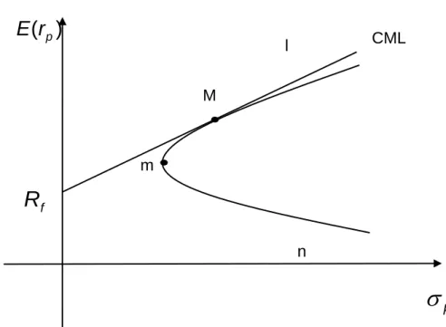
in (2.4) and in (2.5) to solve the optimisation problem would produce a sequence of portfolios on the curve, which represents that the relation between portfolio risk and portfolio return is the mean-variance frontier on the curve lmn in Figure 2.1. The upward-sloping portion of the curve is the efficient frontier (curve lm in Figure 2.1), which provides the best possible trade-off between expected return and risk. These three formulations generate the same efficient frontier. On the efficient frontier, there is the global minimum variance portfolio which has the smallest variance. The point m in Figure 2.1 denotes the global minimum variance portfolio. It can be obtained by solving the optimisation problem:
subject to w'11
which has the solution:
1
Fabozzi et al. (2007) show other commonly used utility functions and conclude that the portfolio optimisation problem is not sensitive to changes of utility function in normal and Student-t distribution. Σw w w ' min (2.6) 1 Σ 1 1 Σ w 1 1 ' m (2.7)
32 2.1.2 Mean-Variance Analysis with Risk-Free Asset and Capital Asset Pricing Model
Building on the mean-variance portfolio theory, Sharpe (1964) and Lintner (1965) design an equilibrium model, the Capital Asset Pricing Model (CAPM), with an assumption of the existence of risk-free assets. The risk-free asset has zero variance. The covariance of the risk-free asset with any risky asset will always equal zero. Their primary assumptions also include:
Investors can borrow or lend at the risk-free rate of return;
All investors will choose an optimal portfolio on the Markowitz efficient frontier;
All investors possess homogeneous expectations;
All investors have the same one period time horizon;
All investments are infinitely divisible;
There are no taxes or transaction costs;
There is no inflation or any change in interest rates; and
Capital markets are in equilibrium.
Suppose that the risk-free asset exists, and that the expected rate of return earned on the risk-free asset is Rf, the rate of return earned on each risky asset is r, the proportion of the portfolio invested in risky portfolio is wr, and
1 w '
1 r is a risk-free asset. The portion of risk-free assets can be positive or negative if risk-free borrowing and lending are allowed. The average rate of return p and the variance
2
p
of the portfolio, when the risk-free asset is combined with the portfolio of risky assets, can be expressed as:
where Σr is the covariance of the risky asset portfolio. The variance of portfolio that combines the risk-free asset with risky assets is the linear proportion of the variance of the risky asset portfolio, because the risk-free asset has zero variance and is uncorrelated with risky assets. From the view of investors, they prefer selecting a portfolio with the highest expected excess return per unit of risk on the efficient frontier. In other words, the Sharpe Ratio (SR), which is
) ) ( ( ' ) ' 1 ( ) ( ' ) ( p r r f f r f p E r w E r w 1R R w Er R (2.8) r r r p w 'Σ w 2 (2.9)
33
calculated as the ratio between expected excess return and standard deviation, could be used to measure portfolio performance, and the optimal portfolio should have the maximal SR. Therefore, in practice, the portfolio problem can also be expressed as the maximisation of the SR:
The solved weights of the investor’s optimal portfolio would be given by:
This optimal portfolio is the tangency portfolio referred to as the market portfolio. We can draw the line from the risk-free rate to the efficient frontier at the point where the line is tangent to the efficient frontier. This line is called the capital market line. The graph of the capital market line is in Figure 2.2. The point M represents the market portfolio. The expression for the capital market line can be shown as:2
where E(rM) is the expected return of the market portfolio, and M is the standard deviation of the market portfolio.
CAPM is a model that determines the expected rate of return on a risky asset
) (ri
E . The systematic risk measure for the individual risky asset is the covariance with the market portfolio Covi,M . The formula for the risk-return relationship is denoted by:
2
The expected variance for a two-asset portfolio is p2 w212(1w)2222w(1w)12; when the risk-free asset is combined with a risky asset portfolio (market portfolio), the expected variance is
2 2 2 M r p w , thus, M p r w
, and the formula (2.8) can be rewritten as formula (2.12).
w Σ w r w w r f R E ' ) ) ( ( ' max (2.10) subject to w'11 ) ) ( ( ' ) ) ( ( 1 1 * f r f r r R E R E r Σ 1 r Σ w (2.11) p M f M f p R r E R r E ) ) ( ( ) ( (2.12)
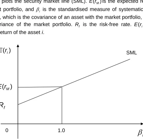
34 i , which is equal to 2, M M i Cov
, is a measure of systematic risk. The market
portfolio has a beta of 1. There is a linear relationship between the expected return and the systematic risk; Figure 2.3 plots the security market line in this linear relationship. In equilibrium, all assets and all portfolios of assets should plot on the security market line.
2.1.3 Criticisms of the Mean-Variance Approach
The simplicity and the intuitive appeal of the mean-variance approach has attracted significant attention from academia and industry. However, contrary to its theoretical reputation, Markowitz’s classical framework has not been used extensively by practitioners as a tool for optimising a large-scale portfolio, due to its numerous implementation difficulties.
The impracticality is that extreme weights or corner solutions from the mean-variance model may be inconvenient in asset allocation, since the investor can neither assign unrealistic weights to each asset, nor diversify risk by investing different assets. Imposing constraints on portfolio weights could alleviate this problem and enable the portfolio to perform better (Frost and Savarino, 1988; Grupa and Eichhorn, 1998; Grauer and Shen, 2000). Discussions regarding the non-short selling constraints can be found in the literature (Jagannathan and Ma, 2003). Additionally, the sensitivity of portfolio weights (Best and Grauer, 1991; Best and Grauer, 1992; Black and Litterman, 1992; Broadie, 1993) is an annoying problem for practitioners as well, as they have to pay significant amounts of transaction costs to buy and sell stocks with weights dramatically changed. The main reason for these problems is the estimation errors in the inputs of the mean-variance model.The accuracy of the estimation of input data will heavily affect the weights allocated to each asset in the mean-variance optimisation, called ‘estimation-error maximisers’ (Michaud, 1989). Michaud argues that the optimised portfolios tend to overweight (underweight) assets
M i M f M f i Cov R r E R r E( ) ( ( )2 ) , (2.13) ( 2, )( ( M) f) M M i f E r R Cov R (2.14) Rf i(E(rM)Rf) (2.15)
35
with large (small) expected returns, negative (positive) correlations and small (large) variances. Merton (1980) demonstrates that historical returns are bad proxies for expected returns. He also demonstrates evidence that the estimated variance and covariance from the historical data will be much more accurate than the corresponding expected return estimates. Similarly, Chopra and Ziemba (1993) verify that the impact of estimation errors on the expected returns on portfolio choice dominates that of estimation errors in variances and covariance. Therefore, they suggest paying attention to estimate, ‘less noisy’ expected returns, followed by a good estimation of variance. To address these problems, robust estimates of the input parameters for optimisation problems become an important research issue. It is advisable to use the Bayes-Stein shrinkage estimator (Jorion, 1985) or the Bayesian estimator (Frost and Savarino, 1986) as alternative estimators of expected return to reduce estimation risk and improve out-of-sample portfolio performance. However, except for estimation error, Green and Hollifield (1992) explain that the high correlation among assets result from the dominance of a single factor in the covariance of asset returns triggering the extreme weights. Therefore, it cannot ignore the impact of correlations on portfolio weights. Fabozzi et al. (2008) suggest using a factor model to model covariance and correlations and therefore deal with the issue of highly correlated assets.
Another significant problem is the computational difficulty associated with inputs of the expected returns and the expected variance-covariance structure for all assets in the investment universe. For example, if there were 100 assets, it would be burdensome for a practitioner to compute 4,950 parameters in the covariance matrix. In practice, it is impossible for portfolio managers to estimate reliable returns for all assets. Estimation errors exist when they anticipate an expected return by using a simple average of historical sample returns. In addition, it is widely agreed that financial asset return volatilities and correlations are time-varying, with persistent dynamics. Asset return volatilities become an important ingredient in many applications, such as portfolio optimisation and market risk measurement. The most popular approach to modelling the conditional covariance matrix of returns is the multivariate GARCH class of models. These models include the Vech and Diagonal Vech models (Bollerslev et al., 1988), the BEKK model (Engle and Kroner, 1995), the