7 0 7 4
|
P a g e
.Inverted Beta Lindley Distribution
N. M. Kilany
1, H. M. Atallah
21
Department of mathematics, Faculty of Science, Menoufia University, Egypt
[email protected]
2Department of mathematics, Faculty of Science, Menoufia University, Egypt
[email protected]
ABSTRACT
In this paper, a three-parameter continuous distribution, namely, Inverted Beta-Lindley (IBL) distribution is proposed and studied. The new model turns out to be quite flexible for analyzing positive data and has various shapes of density and hazard rate functions. Several statistical properties associated with this distribution are derived. Moreover, point estimation via method of moments and maximum likelihood method are studied and the observed information matrix is derived. An application of the new model to real data shows that it can give consistently a better fit than other important lifetime models.
Keywords
Inverted beta distribution; Lindley distribution; Maximum likelihood estimation; Bladder cancer data; Hazard function; Goodness–of–fit.
MATHEMATICS SUBJECT CLASSIFICATION
60E05; 62E101. INTRODUCTION
The beta distribution with support in the standard unit interval (0, 1) has been utilized extensively in statistical theory and practice for over 100 years. It is very versatile and a variety of uncertainties can be usefully modeled by this distribution, since it can take an amazingly great variety of forms depending on the values of its parameters. On the other hand, the inverted beta (IB) distribution with support in (0, ∞) (also known as beta prime distribution or beta distribution of the second kind) can be used to model positive real data. Its probability density function (p.d.f.) with two positive parameters shape parameters and is given by
( )
( ) ( )
(1)
where ( ) ( ) ( ) ( ) is the beta function and ( ) is the gamma function.
The IB distribution has been studied by several authors. McDonald & Richards [14] discussed its properties and obtained the maximum likelihood estimates (MLEs) of the model parameters. The behavior of its hazard ratio function has been examined by McDonald & Richards [13]. Bookstaber & McDonald [2] showed that this distribution is quite useful in the empirical estimation of security returns and in facilitating the development of option pricing models (and other models) that depend on the specification and mathematical manipulation of distributions. Mixtures of two IB distributions have been considered by McDonald & Butler [11] who have applied them in the analysis of unemployment duration. McDonald and
Butler [12] have used this distribution while discussing regression models for positive random variables. Other applications in modeling insurance loss processes have been illustrated by Cummins et al. [3]. McDonaldandBookstaber [10] have developed an option pricing formula based on this distribution that includes the widely used Black Scholes formula based on the assumption of log-normally distributed returns. More recently, Vargo [19] developed moment-ratio diagrams for the IB distribution.
Lindley [9]derived a distribution for modeling waiting times and survival data, which is called later as Lindley distribution (LD). The probability density function of the Lindley distribution is given by:
( ) .
/ ( )
(2)
Ghitany et. al. [4] studied most of the statistical and reliability properties showing that LD afford a better fitting model than the exponential distribution for some cases. Mixture distributions express complex probability distributions in terms of simpler ones, which are the mixture components. They can be used for modeling a statistical population with subpopulations. Using the concept of mixture distributions provides a good model for several types of data with different characteristics. In this paper, we introduce a new distribution having three parameters which is based on mixing the inverted beta distribution and Lindley distributions, so-called the Inverted Beta Lindley distribution (IBL). This paper is organized as follows; Section 2 introduces the Inverted Beta Lindley (IBL) model formulation. The distributional properties of IBL distribution including the hazard and survival functions, the behavior of the probability density function, mean residual life and reversed failure rate, the moments and the associated moments, Lorenz and Bonferroni curves and finally
probability and cumulative function of order statistics are studied in Section 3. Section 4 concerns with the point and interval estimations of IBL distribution. Finally, a real data life application of bladder cancer data are illustrated the potential of IBL distribution compared with other distributions in Section 5.
2. MODEL FORMULATION
The probability density function (p.d.f.) of IBL distribution can be shown as a mixture of Lindley and Inverted Beta distributions as follows
( )
( ) ( )
( )
where,. and ( ) , ( ) are the Lindley and the inverted beta distributions, with density functions given in equations (2) and (1) respectively.
The p.d.f of IBL distribution is defined by:
( )
( )
.
( )
( )
( ) ( )
/
(3)The corresponding cumulative distribution function is
( )
. ( )/ ( ) ( ) ( )̃ ( )
( ) (4) where, ̃( ) ( )
( ) is the regularized hypergeometric function and ( ) ( ) ( ) ( )∑
( ) ( ) ( ( ))
is the hypergeometric function.
3. PROPERTIES OF THE MODEL
In the Section, we discuss some of the main properties of the IBL distribution.
3.1. The Hazard and Survival Functions
The survival function examines the chance of breakdowns of organisms or technical units etc. occur beyond a given point in time. To monitor the lifetime of a unit across the support of its lifetime distribution, the hazard rate is used. The hazard rate measures the tendency to fail or to die depending on the age reached and it thus plays a key role in classifying lifetime distributions. The hazard rate function defined by ( ) ( ) ( )), where ( ) ( ( )) is the survival function. From (3) and (4), the survival and failure (or hazard) rate functions for IBL are obtained by:
( )
( ) ( ) ( ) ̃ ( ) ( ) ( ) (5)( )
( ) ( ) ( ) ( ) ( ) ( ) ( ) ̃ ( ) ( ) (6)3.2. Shapes of the IBL Distribution
In this section, we discuss the possible shapes of the p.d.f. (3) and the hazard rate function (6). It is first observed that
( )
( )
{
( )( )
(
( ) ( ))
,
( )
( )
7 0 7 6
|
P a g e
(a) (b)
(c) (d)
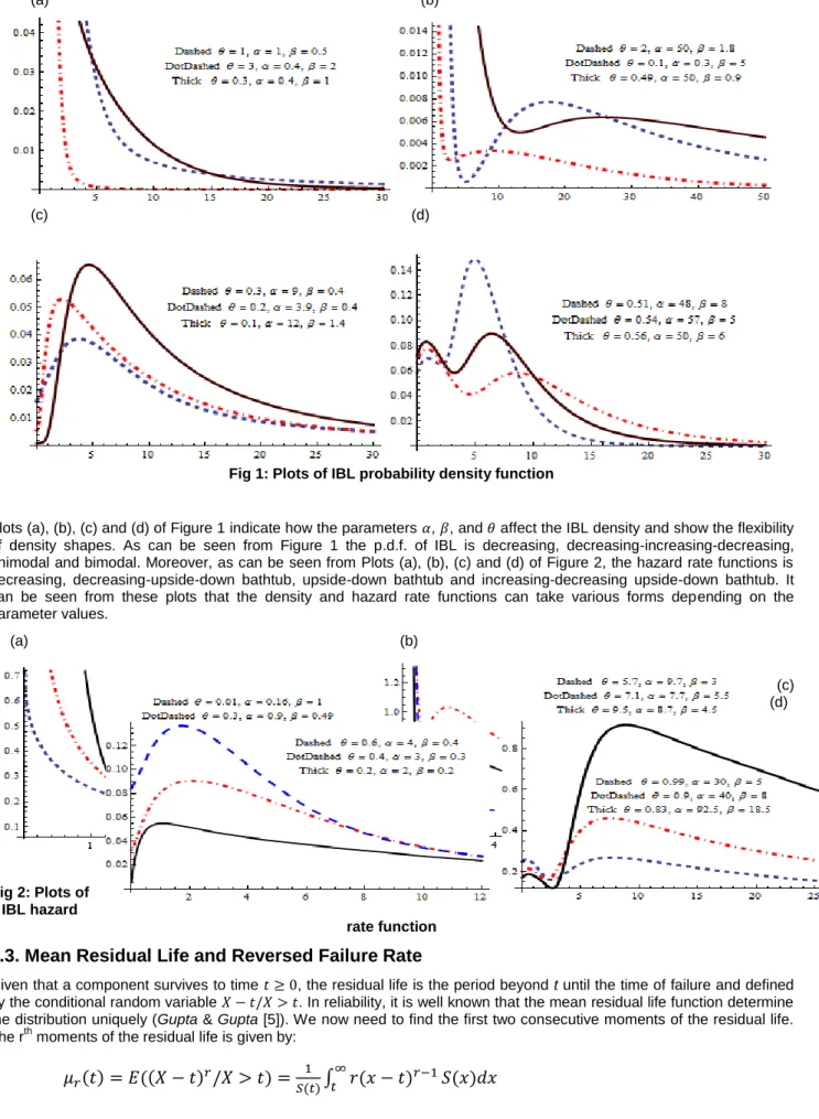
Fig 1: Plots of IBL probability density function
Plots (a), (b), (c) and (d) of Figure 1 indicate how the parameters , , and affect the IBL density and show the flexibility of density shapes. As can be seen from Figure 1 the p.d.f. of IBL is decreasing, decreasing-increasing-decreasing, unimodal and bimodal. Moreover, as can be seen from Plots (a), (b), (c) and (d) of Figure 2, the hazard rate functions is decreasing, decreasing-upside-down bathtub, upside-down bathtub and increasing-decreasing upside-down bathtub. It can be seen from these plots that the density and hazard rate functions can take various forms depending on the parameter values. (a) (b) (c) (d) Fig 2: Plots of IBL hazard rate function
3.3. Mean Residual Life and Reversed Failure Rate
Given that a component survives to time , the residual life is the period beyond t until the time of failure and defined by the conditional random variable . In reliability, it is well known that the mean residual life function determine the distribution uniquely (Gupta & Gupta [5]). We now need to find the first two consecutive moments of the residual life. The rth moments of the residual life is given by:
( ) (( )
)
( )
∫ ( )
The mean residual life (MRL) function of IBL distribution is obtained by the following form
( ) ( )
( )∫ ( )
( ) ( ( ) ( ) ( ) ̃ ( ) ( ) )
( )( ) ( ) ( ) . ( ) ( )( ) ( )/ ( ) ( ) ( )( ( ) ( ) ( ) ̃ ( ) ( ) )
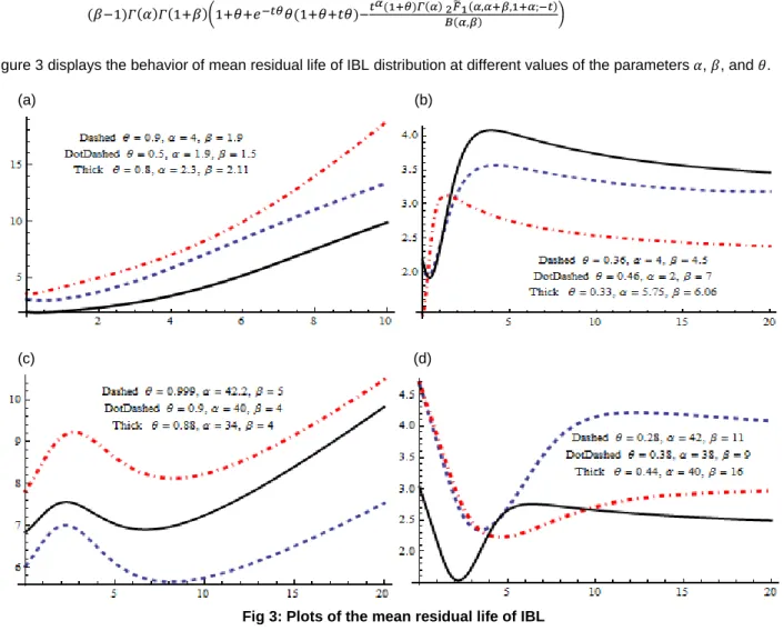
Figure 3 displays the behavior of mean residual life of IBL distribution at different values of the parameters , , and . (a) (b)
(c) (d)
Fig 3: Plots of the mean residual life of IBL
7 0 7 8
|
P a g e
( ) . / ( ) (( )( ) ( ) ( ) ( ) ( ( ) ( ) ( ) ̃( ) ( ) )) ( ( ) ( )( )( ) ( ) ( ) ( ) ( ) ( ) ( ) ( ) ( ( ) ( ) ( ( )) ( ) ( ( )( ( ) ) ( ( ) ( )( )) ( ))))
In addition, in reliability, it is well known that the mean reversed residual life and ratio of two consecutive moments of reversed residual life characterize the distribution uniquely; for more details see Kundu & Nanda [7] and Nanda, et. al.
[17]. The reversed failure for IBL is derived as follows:
( ) ( )
( )
( ) ( ( ) ( ) ( ))
( ( ( ) ( )) ( ) ( ) ( ))
The rth moments of the reversed residual life is given by:
( ) (( )
)
( )
∫ ( )
( )
Thus the mean of the reversed residual life of IBL is given by: ( )
( ) ( ) ( ) ( ) ̃( )
( )
( ( )) ( ) ( ) ̃( )
( )
3.4. Moments and Associated Measures
The first four moments about the origin of IBL distribution are:
( ) ( )
,
( )( )( )( ) ( )( ) ( ) ( ) ( ) ( ) ( ) ( )
,
( ) ( ) ( ) ( ) ( ) ( ) ( )
The second central moments about the mean is given by
( ) ( ( ( ) ) ( )( ) ( ( ) ( ) ) ( )( )( ) ( ( )) ( ) )
Therefore, the mean and variance of IBL are as follows
( )
(
( )
)
and( )
(
( ( ) )
( )( )
( ( ) ( )
)
( )( )( )
( ( ))
( )
)
( )
( )
(
( )
( )
( ) ( ) ( ) ( ) ( )
)
( )
( )
(
( )
( )
( ) ( ) ( ) ( ) ( )
)
where U (a, b, z) is the confluent hypergeometric function.Moreover, the coefficients of variation (CV), skewness ( ) and kurtosis ( ) measures of IBL distribution can be obtained from the expressions respectively
( )√( ( ( ) ) ( )( ) ( ( ) ( ) ) ( )( )( ) ( ( )) ( ) ) ( ( ) ) ( ) √( )
√( ( ( ) ) ( )( ) ( ( ) ( ) ) ( )( )( ) ( ( )) ( ) ) ( ) ( ( ( )) ( ) ( )( )( ) ( ) (( ( ) ( ( )( ( ) ) ) ( )( ) ( ( ) ( ( )) ( ( ( )))) ( )( )( ) ( ( ( ( ( ))))) ( ) ( )( ( ( ( ))) ( ( ( ( )))) ( ( ( ( ))))))))
(
)
( ) ( ) (( )( )( ( ) ) ( ( ) ( )( )( )( )) ( ( )) ( ) ) (( ( ) ( )( )) ( ) ( ( ) ( )( )) ( )( )( )( ) ( ) ( )( )( ) ( )( )( ) ( ) ( ( ) ( )( )) ( )( ) ( )( )( ) ( ( ) ( )( )) ( ( ) ( )( ) ( ( ) ( ) )( ) ( ( ) ( ) ( ) )( ) ( ( ) ( ) ( ) ( ) ) ( ( ) ( ) ( ) ( ) ) ( ( ) ( ) ( ) ( ) ) ( ( ) ( ) ( ) ( ) ) ( ( ) ( ) ( ) ) ))7 0 8 0
|
P a g e
3.5. Lorenz and Bonferroni Curves
The Bonferroni and Lorenz curves have applications not only in economics to study income and poverty, but also in other fields like reliability, demography, insurance and medicine. For IBL distribution, Lorenz and Bonferroni curves are:
, ( )- ( ( ( ))) ( ) ( ) ̃( ) ( ) ( ) and,
( ( ))
( ) ( ( ( ( ))) ( ) ( ) ̃ ( ) ( ) ( ) )( ( ( )) ( ) ( ) ( )̃ ( )The scaled total time on test transform of a distribution function can be written as: ( ( ))
( ) ( ) ( ) ̃( )
( ) ( )
3.6. Probability and Cumulative Function of Order Statistics
The distribution of extreme values plays an important role in statistical applications. In this section the probability and cumulative function of order statistics for IBL distribution are introduced. Suppose is a random sample from IBL distribution. Let denote the corresponding order statistics. The probability density function and the cumulative distribution function of the jth order statistic, say , are given by
( )
( ) ( )* ( )+
* ( )+
( )
( ( ) ( ) ( ) ( ) ) ( ) ( ) ( )
{
( ) ( ) ( ) ̃ ( ) ( ) ( )}
{
. ( )/ ( ) ( ) ̃ ( ) ( ) ( )}
and( ) ∑
(
)
( ) * ( )+
. ( ) ( ) ( )/ ( ( ) . ( ) ( )/ ( ) ( ) ( ) ̃( ) ( ). ( ) ( )/ ( ) ( ) ( ) ̃( )){
( ) ( ) ( ) ̃ ( ) ( ) ( )}
{
. ( )/ ( ) ( ) ̃ ( ) ( ) ( )}
4. ESTIMATION AND INFERENCE
Estimating the unknown parameters of a distribution is essential in applied statistics. In this section, we consider maximum likelihood estimation (MLE) to estimate the involved parameters and the method of moment estimates (MME). Moreover, the asymptotic confidence intervals for the parameters of IBL distribution will be derived using Fisher information matrix.
4.1. Method of Moments Estimates
By equating the first three moments of the population of IBL distribution with the corresponding sample moments, the MME equations are
( )
( )
(7)
( )( ) ( )( ) ( )
(8) ( ) ( ) ( ) ( ) ( ) ( ) ( )
(9) Equations (7), (8), and (9) take the form:
( )
( ) (
)
(10) ( ) ( )( )
( )
( ) ( ) (11) ( )( ) ( )( )( )( )
( ) ( ) (12) From (10) and (11) we obtain,
( ( ) )( ( ) ( ) ( ))
( ( )) ( ) ( ( ) ( ) ( ) ) (13)
( )( ( ) ( ) ( ))
( ( )) ( ) ( ( ) ( ) ( ) ) (14) Substituting from (13) and (14) into (12) we obtain,
(
)
(15) Where, ( ), ( ) ( ) ( ) , ( ) ( ) ( ) , ( ) ( ) ( ) , ( ) ( ) ( ) , ( ) ( ) ( ) , ( ) ( ) ( ) , andSolving equation (15) we can get ̂. In addition, the MME of the other parameters and can be written in terms of ̂ obtained from (15) by substituting in (13) and (14) as follows:
( ̂ ( ̂) )( ̂( ̂) ̂( ̂) ( ))
̂( ̂( ̂)) ̂( ̂) ( ( ̂) ( ̂) ( ̂) )
( ̂)( ̂( ̂) ̂( ̂) ( ))
̂( ̂( ̂)) ̂( ̂) ( ( ̂) ( ̂) ( ̂) )
4.2. Maximum Likelihood Estimates
The method of maximum likelihood consists of maximizing the likelihood function with respect to the parameters . Let be a random sample of size n from inverted beta-Lindley distribution with p.d.f. (3), the log-likelihood function of IBL is given by:
( ) ( ) ∑
(
(
)
( )
(
)
( )
)
It follows that the maximum likelihood estimators (MLEs), say ̂, ̂ and ̂ are the simultaneous solutions of the equations. Differentiation of ( ) with respect to yields;
( )
∑
( )( (
) (
) ( ) ( ))
( )
( )
(
)
7 0 8 2
|
P a g e
( )
∑
( )( (
) ( ) ( ))
( )
( ) (
)
( )
∑
( ) (
)
(
)
( )
( )
(
)
where ( )is the digamma function given by ( ) ( ) ( ). The solution of this nonlinear system of equations has not closed form and need to be solved numerically. Certain numerical iterative techniques may be used for estimating the parameters and the global maxima of the log-likelihood can be investigated by setting different starting values for the parameters.
In order to determine confidence intervals for the distribution parameters, we need the information matrix. The elements of the 3× 3 observed information matrix ( ) are given by:
( ( ))
(
( )( ) ( ( )) ( ( ) ( ) ( )) ( . ( ( ))/) ( ) ( ) ( ))
( ( ))
( )
(
( ) ( )
( ))
(
( ) .
( )( )
( )( )/
( )
( ) .( ( ) ( ))
( ( ) ( ))( ( ) ( ) ( ) ( ))
( )( )
( )
( )/)
( ( ))
( ) . ( ) ( ) ( )/
( ( )
( )( ( ) ( ) ( ))
.
( ) ( )
( )/ .
( )( )
( )( )/)
( ( ))
( ) ( ( )) ( )( ( ) ( ) ( ) ( )) ( ( ) ( ) ( ))
( ( ))
( ) ( ( )) ( )( ( ) ( ) ( )) ( ( ) ( ) ( ))
( ( ))
( )
(
( ) ( )
( ))
( ( )
( ) .( ( ) ( )
( ))( ( ) ( ) ( ) ( ))
( )( )/
( )
( )( ))
where ( )( ) is the ploygamma function of order n defined as is the n-th derivative of the digamma function. Under conditions that are fulfilled such as the parameters lying in the interior of the parameter space but not on the boundary, the asymptotic distribution of √ ( ̂ ) is ( ( )), where I( ) = E{ J( ) } is the expected information matrix. The approximate multivariate normal distribution ( ( )), where ( ) is the inverse observed information matrix evaluated at ̂ be used to determine approximate confidence intervals for the distribution parameters.
5. APPLICATION
Consider a data set corresponding to remission times (in months) of a random sample of 128 bladder cancer patients given in Lee & Wang [8]. The data are given as follows: 0.08, 2.09, 3.48, 4.87, 6.94, 8.66, 13.11, 23.63, 0.20, 2.23, 3.52, 4.98, 6.97, 9.02, 13.29, 0.40, 2.26, 3.57, 5.06, 7.09, 9.22, 13.80, 25.74, 0.50, 2.46, 3.64, 5.09, 7.26, 9.47, 14.24, 25.82, 0.51, 2.54, 3.70, 5.17, 7.28, 9.74, 14.76, 26.31, 0.81, 2.62, 3.82, 5.32, 7.32, 10.06, 14.77, 32.15, 2.64, 3.88, 5.32, 7.39, 10.34, 14.83, 34.26, 0.90, 2.69, 4.18, 5.34, 7.59, 10.66, 15.96, 36.66, 1.05, 2.69, 4.23, 5.41, 7.62, 10.75, 16.62, 43.01, 1.19, 2.75, 4.26, 5.41, 7.63, 17.12, 46.12, 1.26, 2.83, 4.33, 5.49, 7.66, 11.25, 17.14, 79.05, 1.35, 2.87, 5.62, 7.87, 11.64, 17.36, 1.40, 3.02, 4.34, 5.71, 7.93, 11.79, 18.10, 1.46, 4.40, 5.85, 8.26, 11.98, 19.13, 1.76, 3.25, 4.50, 6.25, 8.37, 12.02, 2.02, 3.31, 4.51, 6.54, 8.53, 12.03, 20.28, 2.02, 3.36, 6.76, 12.07, 21.73, 2.07, 3.36, 6.93, 8.65, 12.63, 22.69. We have fitted the IBL distribution to the dataset using MLE. The proposed Inverted Beta-Lindley distribution is compared with the inverted beta (IB), Lindley (LD) and the following models:
The Beta Exponentiated Pareto (BEP) distribution Zea et al. [20] with density function,( )
( )( .
/
)
( ( .
/
)
)
The Beta Pareto (BP) distribution Akinsete et al. [1] with density function,( )
( )
( .
/
)
.
/
The Exponentiated Pareto (EP) distribution Gupta et al. [6] with density function,( )
( .
/
)
The Pareto distribution with density function,( )
The Beta Exponential (BE) distribution Nadarajah & Kotz [16] with density function, ( ) ( )( )
The Beta Lindley (BL) distribution Merovci & Sharma [15] with density function, ( ) ( ) ( )
( )( )
.
/
The Gamma distribution with density function,
( )
⁄( )
The Beta Transmuted Weibull (BTW) distribution Pal & Tiensuwan [18] with density function,( )
( ).
/ .
/ .
/
( .
/ .
/)
| |
To verify the goodness of fit of certain statistical models, some goodness-of-fit statistics shall be used. They are computed using the symbolic computation package Mathematica. The following goodness-of-fit statistics are considered: the log-likelihood function evaluated at the MLEs, the Akaike information criterion (AIC), the Bayesian information criterion
7 0 8 4
|
P a g e
(BIC),the consistent Akaike information criteria (CAIC) and the Kolmogorov Smirnov (K-S) statistics. These statistics are utilized to evaluate how closely a specific distribution with a given cumulative distribution function fits the corresponding empirical distribution for a given data set. The distribution having the better fit will be the one whose goodness-of-fit statistic is the smallest. The AIC, BIC, CAIC are given by
( ̂)
( ̂) ( )
( ̂)
where ( ̂) denotes the log-likelihood function evaluated at the maximum likelihood estimates for parameters , q is the number of parameters, and n is the sample size.
Table 1. MLEs for estimates for different distributions Distribution MLEs ̂ ̂ ̂ ̂ ̂ ̂ ̂ IBL 0.4933 17.625 2.356 - - - - BTW - 0.2133 0.9999 0.9762 - 1.5266 0.3269 BL 1.861 1.340 0.065 - - - - BE - 1.149 0.997 0.116 - - - Gamma - - - 7.9876 1.1725 - - Lindley 0.196 - - - - BEP - 8.6121 0.080 - 0.0508 0.3477 159831 IB - 1.200 0.700 - - - - BP - - 0.080 - 0.0109 4.8049 100.500 EP - 4.1518 0.080 - 0.4722 - - Pareto - - 0.080 - 0.1519 - -
The maximum likelihood method is used for estimating the parameters of all the compared distributions and the parameter estimates are given in Tables 1. Further, all the aforementioned goodness-of-fit statistics are determined for each distribution and listed in Table 2. It can be observed from Table 2 that the IBL distribution has the smallest statistics. Accordingly, we can conclude that the IBL distribution represents the best fit among the compared distributions.
Table 2. Goodness-of-Fit Statistics for the remission times of bladder cancer data
Distribution Measures
-Log L AIC BIC CAIC K-S
IBL 409.67 825.35 833.91 825.55 0.0381 BTW 409.86 829.73 843.87 830.23 0.0399 BL 412.80 831.60 840.16 831.79 0.0937 BE 413.19 832.37 840.93 832.57 0.0652 Gamma 413.37 830.74 836.44 830.83 0.0733 Lindley 419.53 841.06 843.91 841.09 0.1087 BEP 433.40 874.80 886.20 875.10 0.1427 IB 468.08 940.15 945.86 940.25 0.3747 BP 482.35 970.70 979.20 970.90 0.2231 EP 494.10 992.20 997.90 992.30 0.2515 Pareto 593.65 1189.30 1192.10 1189.30 0.3729
Conclusion
We propose a new distribution, so-called the Inverted Beta- Lindley (IBL) distribution, and study some of its general structural properties and statistical measures. This distribution has the support on the positive real line and it can be used to analyze lifetime data. The shapes and some properties of probability density and hazard functions are provided. The distribution exhibits a wide range of hazard shaped. The estimation of the model parameters is approached by method of moments and maximum likelihood. Moreover, the Fisher information matrix for interval estimation is studied for IBL
distribution. A real data on bladder cancer is used to illustrate and compare the potential of IBL distribution with other competing distributions showed that it has a superior performance among the compared distributions as evidenced by some goodness-of-fit tests.
REFERENCES
1. Akinsete, A., Famoye, F. and Lee, C. (2008). “The Beta-Pareto Distribution”. Statistics, 42(6), 547-563.
2. Bookstaber, R.M. and McDonald, J.B. (1987). “A General Distribution for Describing Security Price Returns”. The Journal of Business, 60,401–424.
3. Cummins, J.D., Dionne, G., McDonald, J.B. and Pritchett, B.M. (1990). “Applications of The GB2 Family of Distributions in Modeling Insurance Loss Processes”. Insurance: Mathematics and Economics, 9, 257–272. 4. Ghitany, M.E., Atieh, B. and Nadarajah, S. (2008). “Lindley Distribution and its Application”. Mathematics and
Computer in Simulation, 78:493–506.
5. Gupta, P.L. and Gupta, R.C. (1983). “On the Moments of Residual life in Reliability and some Characterization Results”. Communications in Statistics-Theory and Methods, 12(4), 449-461.
6. Gupta, R. C., Gupta, R. D. and Gupta, P. L. (1998). “Modeling Failure Time Data by Lehman Alternatives”. Communications in Statistics: Theory and Methods, 27, 887-904.
7. Kundu, C. and Nanda, A.K. (2010). “Some Reliability Properties of the Inactivity Time”. Communications in Statistics-Theory and Methods, 39, 899-911.
8. Lee E. T. and Wang, J. W. (2003). “Statistical Methods for Survival Data Analysis”. John Wiley & Sons, New York, NY, USA, 3rd edition.
9. Lindley, D. V. (1958). “Fiducial Distributions and Bayes' Theorem”. Journal of the Royal Statistical Society, Series B, 20(1), 102–107.
10. McDonald, J.B. and Bookstaber, R.M. (1991). “Option Pricing for Generalized Distributions”. Communications in Statistics–Theory and Methods, 20, 4053–4068.
11. McDonald, J.B. and Butler, R.J. (1987). “Some Generalized Mixture Distributions with an Application to Unemployment Duration”. The Review of Economics and Statistics, 69, 232–240.
12. McDonald, J.B., Butler, R.J. (1990). “Regression models for positive random variables”. Journal of Econometrics, 43:227–251.
13. McDonald, J.B. and Richards, D.O. (1987). “Hazard Rates and Generalized Beta Distribution”. IEEE Transactions on Reliability, 36, 463–466.
14. McDonald, J.B. and Richards, D.O. (1987). “Model Selection: Some Generalized Distributions”. Communications in Statistics–Theory and Methods, 16, 1049–1074.
15. Merovci, F. and Sharma, V.K. (2014). “The Beta-Lindley Distribution: Properties and Applications”. Journal of Applied Mathematics, 10, 198-951.
16. Nadarajah, S. and Kotz, S. (2006). “The Beta Exponential Distribution”. Reliability Engineering and System Safety, 91, 689–697.
17. Nanda, A.K., Singh, H. and Misra, N., Paul, P. (2003). “Reliability Properties of Reversed Residual Lifetime”. Communications in Statistics-Theory and Methods, 32(10), 2031-2042.
18. Pal, M. and Tiensuwan, M. (2014). “The Beta Transmuted Weibull Distribution”. Austrian Journal of Statistics, 43(2), 133–149.
19. Vargo, E., Pasupathy, R. and Leemis, L. (2010). “Moment-Ratio Diagrams For Univariate Distributions”. Journal of Quality Technology, 42:276–286.
20. Zea, L.M., Silva, R.B, Bourguignon, M., Santos, A.M. and Cordeiro, G.M. (2012). “The Beta Exponentiated Pareto Distribution with Application to Bladder Cancer Susceptibility”. International Journal of Statistics and Probability, 2, 1927-7032.