Exploring the topology of complex phylogenomic and transcriptomic networks

(1)

by

Deborah A. Weighill

Thesis presented in partial fullment of the requirements for

the degree of Master of Science in Wine Biotechnology in the

Faculty of AgriScience at Stellenbosch University

Institute for Wine Biotechnology, University of Stellenbosch,

Private Bag X1, Matieland 7602, South Africa.

Supervisor: Dr. D.A. Jacobson

(2)

The nancial assistance of the National Research Foundation (NRF) towards this research is hereby acknowledged. Opinions expressed and conclusions arrived at, are those of the author and are not necessarily to be attributed to the NRF.

i

(3)

Declaration

By submitting this thesis electronically, I declare that the entirety of the work contained therein is my own, original work, that I am the sole author thereof (save to the extent explicitly otherwise stated), that reproduction and pub-lication thereof by Stellenbosch University will not infringe any third party rights and that I have not previously in its entirety or in part submitted it for obtaining any qualication.

11/08/2014

Date: . . . .

(4)

Abstract

Exploring the Topology of Complex Phylogenomic and

Transcriptomic Networks

D.A. Weighill

Institute for Wine Biotechnology, University of Stellenbosch,

Private Bag X1, Matieland 7602, South Africa.

Thesis: MSc Wine Biotechnology (Computational Biology) December 2014

This thesis involved the development and application of network approaches for the construction, analysis and visualization of phylogenomic and transcrip-tomic networks.

A co-evolutionary network model of grapevine genes was constructed based on three mechanisms of evolution. The investigation of local neighbourhoods of this network revealed groups of functionally related genes, illustrating that the multi-mechanism evolutionary model was identifying groups of potentially co-evolving genes.

An extended network denition, namely 3-way networks, was investigated, in which edges model relationships between triplets of objects. Strategies for weighting and pruning these 3-way networks were developed and applied to a phylogenomic dataset of 211 bacterial genomes. These 3-way bacterial net-works were compared to standard 2-way network models constructed from the same dataset. The 3-way networks modelled more complex relationships and revealed relationships which were missed by the two-way network models. Network meta-modelling was explored in which global network and node-by-node network comparison techniques were applied in order to investigate the eect of the similarity metric chosen on the topology of multiple types of networks, including transcriptomic and phylogenomic networks. Two new net-work comparison techniques were developed, namely PCA of Topology Proles and Cross-Network Topological Overlap. PCA of Topology Proles compares

(5)

networks based on a selection of network topology indices, whereas Cross-Network Topological Overlap compares two networks on a node-by-node level, identifying nodes in two networks with similar neighbourhood topology and thus highlighting areas of the networks with conicting topologies. These net-work comparison methods clearly indicated how the similarity metric chosen to weight the edges of the network inuences the resulting network topology, consequently inuencing the biological interpretation of the networks.

(6)

Uittreksel

Exploring the Topology of Complex Phylogenomic and

Transcriptomic Networks

(Exploring the Topology of Complex Phylogenomic and Transcriptomic Networks)

D.A. Weighill

Instituut Wynbiotegnologie, Universiteit van Stellenbosch,

Privaatsak X1, Matieland 7602, Suid Afrika.

Tesis: MSc Wyn Biotegnologie Desember 2014

Hierdie tesis hou verband met die ontwikkeling en toepassing van netwerk benaderings vir die konstruksie, analise en visualisering van logenomiese en transkriptomiese netwerke.

'n Mede-evolusionrê netwerk model van wingerdstok gene is gebou, gebaseerd op drie meganismes van evolusie. Die ondersoek van plaaslike omgewings van die netwerk het groepe funksioneel verwante gene aan die lig gebring, wat daarop dui dat die multi-meganisme evolusionêre model groepe van potensi-eele mede-evolusieerende gene identiseer.

'n Uitgebreide netwerk denisie, naamliks 3-gang netwerke, is ondersoek, waarin lyne die verhoudings tussen drieling voorwerpe voorstel. Strategieë vir weeg en snoei van hierdie 3-gang netwerke was ontwikkel en op 'n logenomiese datastel van 211 bakteriële genome toegepas. Hierdie 3-gang bakteriële netwerke is met die standaard 2-gang netwerk modelle wat saamgestel is uit dieselfde datastel vergelyk. Die 3-gang netwerke het meer komplekse verhoudings gemodelleer en het verhoudings openbaar wat deur die tweerigting-netwerk modelle gemis is.

Verder is netwerk meta-modellering ondersoek waarby globalle netwerk en punt-vir-punt netwerk vergelykings tegnieke toegepas is, met die doel om die eek van die ooreenkoms-maatstaf wat gekies is op die topologie van verskeie tipes netwerke, insluitend transcriptomic en logenomiese netwerke, te bepaal.

(7)

Twee nuwe netwerk-vergelyking tegnieke is ontwikkel, naamlik PCA of Topo-logy Proles en Cross-Network Topological Overlap. PCA van Topologie Proele vergelyk netwerke gebaseer op 'n seleksie van netwerk topologie in-dekse, terwyl Cross-netwerk Topologiese Oorvleuel vergelyk twee netwerke op 'n punt-vir-punt vlak, en identiseer punte in twee netwerke met soortgelyke lokale topologie en dus lê klem op gebiede van die netwerke met botsende topologieë. Hierdie netwerk-vergelyking metodes dui duidelik aan hoe die oor-eenkoms maatstaf wat gekies is om die lyne van die netwerk gewig te gee, die gevolglike netwerk topologie beïnvloed, wat weer die biologiese interpretasie van die netwerke kan beïnvloed.

(8)

Acknowledgements

I would like to acknowledge Carissa Blekker and Piet Jones for assistance in the translation of the Abstract to Afrikaans, Piet Jones and Armin Geiger for useful discussions, as well as Daniel Jacobson for supervision, input, advice and support.

(9)

Dedications

To Tom, Malley, Dan and Ralph - Husband, companion, friend and bar.

(10)

List of Figures

2.1 An Example Network. (a) Visualization of the network drawn as nodes (circles) connected by edges (lines) (b) The corresponding unweighted adjacency matrix. . . 3 2.2 Canberra Distance vs. Czekanowski Similarity A visual aid

in the relatedness of the Czekanowski similarity index and the Can-berra distance. . . 8 2.3 Visualization of the MCL process. Repeated rounds of

expan-sion and ination promote paths strong ow and remove paths of weak ow, resulting in clusters. (From [38].) . . . 17 2.4 Graphlets. All possible 3, 4 and 5 node graphlets. (From [42].) . . 19 2.5 Levels Of Orthology Numbers generated by LOFT.

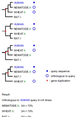
Hierar-chical LOFT numbers assigned to genes from a section of COG4565. Red square nodes represent gene duplication events and green di-amond nodes represent speciation events are represented as green diamonds. (From [52].) . . . 23 2.6 RIO Bootstrap Scores. A simple example in which RIO is used

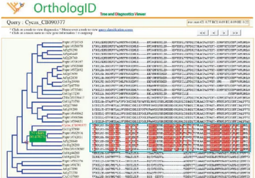
to determine orthologs of a human gene using 4 bootstrap resam-ples. (From [53].) . . . 24 2.7 OrthologID Interface. The visual interface of OrthologID

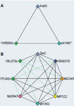
show-ing the charactieristic amino acids for a family highlighted in red. (Modied from [54].) . . . 25 2.8 Clusters of Orthologous Groups (a) A Best Hit Triangle, the

building block of COGs (b) COG constructed by merging triangles. (Modied from [59].) . . . 26 2.9 TribeMCL Flow diagram of the TribeMCL pipeline. (From [39].) . 27 2.10 InParanoid Clustering. Seed orthologs (A1 and B1) form the

centers of clusters and inparalogs clustered around orthologs if they have a similarity score greater than or equal to the similarity be-tween the two seed orthologs. (From [65].) . . . 28 2.11 InParanoid Cluster Merging. Approaches for merging, deleting

or dividing overlapping clusters around seed orthologs. (From [65].) 29 2.12 InParanoid Condence Scores. Range of condence scores

as-signed to inparalogs indicating their relative similarity to the main ortholog. (From [65].) . . . 30

(14)

2.13 OrthoMCL Pipeline. Flow diagram for the OrthoMCL pipeline. (From [56]). . . 31 2.14 Coorthologs. Coorthologs rened as genes in two dierent species

which are connected transitively through an orthologous ship, indicated by solid black lines, and an inparalogous relation-ship,indicated by dotted black lines. (From [67].) . . . 31 2.15 Estimated Sensitivity and Specicity. The false negative (FN)

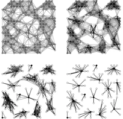
rate and false positive (FP) rate of dierent orthology detection methods estimated using latent class analysis. (From [67].) . . . 32 2.16 Shared Gene Network. Network of gene sharing for various

organisms. Each node represents a genome. Green nodes represent cellular genomes, purple nodes represent plasmid genomes and red nodes represent phage genomes. Nodes are connected based on shared gene content. (From [79].) . . . 35 2.17 ContextMirror Method. Flow diagram for the ContextMirror

Method. (From [80].) . . . 36 2.18 Co-expression Module Comparison. General pipeline for the

determination of co-expression modules conserved across species. (From [84].) . . . 38 2.19 MATISSE Gene Modules. Nodes are clustered into modules

based on topological connectedness in the interaction network indi-cated by solid black lines and expression prole similarity indiindi-cated by dotted grey lines. (From [86].) . . . 39 3.1 Methods Summary. Summary of the workow used for

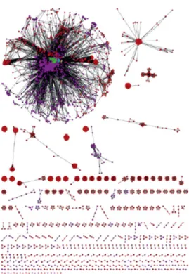
con-structing the co-evolution networks. . . 7 3.2 Combined Co-evolution Network. (A) Network of signicant

overlaps between all three types of co-evolution modules. This net-work was constructed by merging the netnet-works from Supplementary Figures S2, S3 and S4. Each node represents a module of poten-tially co-evolving genes: Blue nodes represent gene co-expression modules, pink nodes represent ERC modules and yellow nodes rep-resent gene family modules. Edges (lines between nodes) reprep-resent signicant overlaps between co-evolution modules. (B) Number of grapevine gene pairs that are co-evolving in terms of 1, 2 and 3 mechanisms of evolution. (C) Number of grapevine genes that are evolving in terms of 1, 2 and 3 mechanisms of evolution. . . 9 3.3 Linked Subnetworks. Subnetworks 1, 2 and 4 combined to

pro-duce a connected network. All three of these subnetworks showed enrichment in defense-related functions and are in close proximity in the combined overlap network. . . 16

(15)

3.4 Quasi-pathway. Network of the main functions present in the links between subnetworks 1, 2 and 4 and the genes associated with those functions. Purple nodes represent genes, green nodes represent GO terms. Edges link GO terms to genes associated with those terms or link GO terms in close proximity in the GO hierarchy. 17 S1 Co-expression-ERC Co-evolution Network. Network of

sig-nicant overlaps between co-expression modules (blue nodes) and ERC modules (pink nodes). Edges represent signicant overlaps between the co-expression modules and the ERC modules. . . 24 S2 ERC-Gene family Co-evolution Network. Network of

signif-icant overlaps between ERC modules (pink nodes) and gene fam-ily correlation modules (yellow nodes). Edges represent signicant overlaps between the ERC modules and gene family modules. . . . 25 S3 Co-expression-Gene family Co-evolution Network. Network

of signicant overlaps between co-expression modules (blue nodes) and gene family correlation modules (yellow nodes). Edges rep-resent signicant overlaps between the co-expression modules and gene family modules . . . 26 S4 Distributions (A) Power Law Distrbution (B) Degree

Distribu-tion for the combined co-evoluDistribu-tion network. A property of scale-free networks is that their degree distribution follows a power-law distribution. This gure illustrates that the combined co-evolution network is scale-free, since its degree distribution is similar to the power law distribution. . . 27 S5 Subnetworks. (A) Subnetwork 1 consists of a central gene

fam-ily correlation module (yellow node) intersecting with several co-expression modules (blue nodes) and one ERC module (pink node). (B) Subnetwork 2 consists of a central co-expression module (blue node) surrounded by several gene family modules (yellow nodes), ERC modules (pink nodes) and one other co-expression module. (C) Subnetwork 3 consists of a central ERC module intersecting with several co-expression modules and gene family modules. (D) Subnetwork 4 consists of a central gene family module surrounded by several co-expression modules and ERC modules. . . 28 S6 Co-evolving Functions. Summary of the related functions which

are enriched in (A) subnetwork 2 and (B) subnetwork 4. Arrows indicate relationships for which there is previous literature evidence as referred to in the text. . . 29 S7 Node Enrichment View: Subnetwork 1. GOEAST results

for the node enrichment view of subnetwork 1. Yellow rectangles indicate enriched GO terms. Arrows indicate relationships between terms in the Gene Ontology and are red if both terms are enriched, black if one of terms connected by the arrow is enriched or dashed if nether term connected is enriched. . . 30

(16)

S8 Edge Enrichment View: Subnetwork 1. GOEAST results for the node enrichment view of subnetwork 1. Yellow rectangles indicate enriched GO terms. Arrows indicate relationships between terms in the Gene Ontology and are red if both terms are enriched, black if one of terms connected by the arrow is enriched or dashed if nether term connected is enriched. . . 30 S9 Node Enrichment View: Subnetwork 2. GOEAST results

for the node enrichment view of subnetwork 2. Yellow rectangles indicate enriched GO terms. Arrows indicate relationships between terms in the Gene Ontology and are red if both terms are enriched, black if one of terms connected by the arrow is enriched or dashed if nether term connected is enriched. . . 31 S10 Edge Enrichment View: Subnetwork 2. GOEAST results

for the node enrichment view of subnetwork 2. Yellow rectangles indicate enriched GO terms. Arrows indicate relationships between terms in the Gene Ontology and are red if both terms are enriched, black if one of terms connected by the arrow is enriched or dashed if nether term connected is enriched. . . 31 S11 Combined Enrichment View: Subnetwork 2. MultiGOEAST

results combining the node enrichment view and edge enrichment view of subnetwork 2. Yellow rectangles represent GO terms which are enriched in both the edge and the node view, green rectangles represent GO terms only enriched in the edge view and red rect-angles represent GO terms only enriched in the node view. Arrows indicate relationships between terms in the Gene Ontology and are red if both terms are enriched, black if one of terms connected by the arrow is enriched or dashed if nether term connected is enriched. 32 S12 Node Enrichment View: Subnetwork 3. GOEAST results

for the node enrichment view of subnetwork 3. Yellow rectangles indicate enriched GO terms. Arrows indicate relationships between terms in the Gene Ontology and are red if both terms are enriched, black if one of terms connected by the arrow is enriched or dashed if nether term connected is enriched. . . 32 S13 Edge Enrichment View: Subnetwork 3. GOEAST results

for the node enrichment view of subnetwork 3. Yellow rectangles indicate enriched GO terms. Arrows indicate relationships between terms in the Gene Ontology and are red if both terms are enriched, black if one of terms connected by the arrow is enriched or dashed if nether term connected is enriched. . . 33

(17)

S14 Node Enrichment View: Subnetwork 4. GOEAST results for the node enrichment view of subnetwork 4. Yellow rectangles indicate enriched GO terms. Arrows indicate relationships between terms in the Gene Ontology and are red if both terms are enriched, black if one of terms connected by the arrow is enriched or dashed if nether term connected is enriched. . . 33 S15 Edge Enrichment View: Subnetwork 4. GOEAST results

for the node enrichment view of subnetwork 4. Yellow rectangles indicate enriched GO terms. Arrows indicate relationships between terms in the Gene Ontology and are red if both terms are enriched, black if one of terms connected by the arrow is enriched or dashed if nether term connected is enriched. . . 34 S16 Combined Enrichment View: Subnetwork 4. MultiGOEAST

results combining the node enrichment view and edge enrichment view of subnetwork 4. Yellow rectangles represent GO terms which are enriched in both the edge and the node view, green rectangles represent GO terms only enriched in the edge view and red rect-angles represent GO terms only enriched in the node view. Arrows indicate relationships between terms in the Gene Ontology and are red if both terms are enriched, black if one of terms connected by the arrow is enriched or dashed if nether term connected is enriched. 34 S17 Hormone Crosstalk Quasi-Pathway Network of genes present

in subnetwork 11 (purple nodes) which are connected to at least 2 of selected GO-terms (light green nodes). This network indicates the crosstalk between biotic and abiotic stress responses through hormone signalling on a gene level, as suggested by the enrichment in subnetwork 4. . . 35 S18 Breadth rst search Subnetwork of Figure S17, constructed by

selecting all nodes within a breadth rst search of length 2 from the node "defense response to bacteria". . . 36 S19 Crosstalk Gene-Module Network Network of genes (purple

nodes) from Figure S18 connected to co-evolution modules in which they are present. In the case of gene family modules, genes are con-nected to the gene families in which they are present, and the gene families are connected to the gene family modules in which they are present. Yellow nodes represent gene family modules, light orange nodes represent gene families, blue nodes represent co-expression modules an pink nodes represent ERC modules. . . 37 S20 Merged Crosstalk Network Merged gene-go network from

Fig-ure S18 and gene-module network from FigFig-ure S19. Purple nodes represent genes, light green nodes represent GO-terms, yellow nodes represent gene family modules, light orange nodes represent gene families, blue nodes represent co-expression modules an pink nodes represent ERC modules . . . 38

(18)

S21 Linking Nodes. Network of nodes linking subnetworks 1, 2 and 4. Yellow and blue nodes represent co-expression and gene-family modules respectively, and green nodes represent GO-terms. . . 39 4.1 3-way Edges and Intersections (a) A small, 3-way network

con-sisting of 5 nodesv1, v2, v3, v4 andv5 and two 3-way edgese1ande2.

Edge e1 connects nodes v3, v4 and v5 and edge e2 connects nodes

v1, v2 and v3. (b) Venn diagram for a 3-way intersection of species.

a is the number of families present in species A, b is the number

of families present in speciesB, cis the number of families present

in species C, ab is the number of families present in species A and

species B, ac is the number of families present in species A and

species C, bc is the number of families present in species B and

speciesC,abcis the number of families present in speciesA,B and

C, ¯a is the number of families present only in species A, ¯b is the

number of families present only in species B and ¯c is the number

of families present only in species C. . . 4

4.2 Best-Edges 3-way Sørensen Network. 3-way Sørensen net-work pruned by selecting the best and second best edge for each node. Nodes represent bacterial species and edges represent sim-ilarity between triplets of bacterial species based on gene family content, quantied using the 3-way Sørensen Index. Nodes are coloured according to genus. Default colour is grey. . . 10 4.3 2-way Sørensen Networks (a) 2-way Sørensen Best Edges

Net-work (b) Maximum Spanning Tree (MST) of the all-vs-all Sørensen network. Nodes represent bacterial species and edges represent sim-ilarity between pairs of bacterial species based on gene family con-tent, quantied using the 3-way Sørensen Index. Nodes are coloured according to genus. The same node colour key as in Figure 2 applies. 15 4.4 Best-Edges 3-way Czekanowski Network 3-way Czekanowski

network pruned by selecting the best and second best edge for each node. Nodes represent bacterial species and edges represent sim-ilarity between triplets of bacterial species based on gene family content, quantied using the 3-way Czekanowski Index. Nodes are coloured according to genus. The same node colour key as in Figure 2 applies. . . 16 4.5 2-way Czekanowski Networks (a) 2-way Czekanowski Best Edges

Network (b) Maximum Spanning Tree (MST) of the all-vs-all Czekanowski network. 3-way Sørensen network pruned by selecting the best and second best edge for each node. Nodes represent bacterial species and edges represent similarity between pairs of bacterial species based on gene family content, quantied using the 3-way Sørensen Index. Nodes are coloured according to genus. The same node colour key as in Figure 2 applies. . . 17

(19)

4.6 Shared Enriched Families Network of bacteria species connected through shared enriched gene families. Small, white nodes represent gene families, coloured nodes represent bacterial species coloured by genus. Edges connect gene families to species in which they are enriched. . . 18 4.7 Clostridium and Bacillus subnetwork. Subnetworks

contain-ing the Clostridium and Bacillus species selected from (a) 3-way best edge Sørensen Network (b) 3-way best edge Czekanowski Net-work (c) Gene family enrichment netNet-work. . . 19 4.8 Clustering within Brucella genus. Subnetworks containing

Brucella species constructed by selecting Brucella species and all neighbouring species nodes from (a) 3-way best edge Sørensen Net-work (b) 3-way best edge Czekanowski NetNet-work (c) Gene family enrichment network. . . 20 4.9 Separation of Rhodobacter species. Subnetworks containing

Rhodobacter species constructed by selecting Rhodobacter species and all neighbouring species nodes from (a) 3-way best edge Sørensen Network (b) 3-way best edge Czekanowski Network (c) Gene family enrichment network. . . 21 4.10 Rhodobacter and Brucella species. Subnetworks containing

Brucella and Rhodobacter species constructed by selecting Bru-cella and Rhodobacter species and all neighbouring species nodes from (a) 3-way best edge Czekanowski Network (b) Gene family enrichment network. . . 22 S1 Thresholded 3-way Sørensen Network Network constructed

by setting a 0.76 threshold for the 3-way Sørensen Network, and removing all 3-way edges below this threshold. . . 28 S2 Thresholded 3-way Czekanowski NetworkNetwork constructed

by setting a 0.76 threshold for the 3-way Czekanowski Network, and removing all 3-way edges below this threshold. . . 29 S3 3-Way Edges Close-up of a section of the thresholded 3-way

net-work showing the 3-way edges. Large, coloured nodes represent bacterial species, whereas small white nodes and their respective 3 edges represent 3-way edges connecting the bacterial nodes. . . 30 S4 Union Sørensen MST and Sørensen 3-way Best Edge

Net-work. Network constructed by taking the union of the Sørensen 3-way Best Edge Network (Figure 2) and the Sørensen MST (Figure 3b). . . 31 S5 Union Czekanowski MST and Czekanowski 3-way Best Edge

Network Network constructed by taking the union of the Czekanowski 3-way Best Edge Network (Figure 4) and the Czekanowski MST (Figure 5b). . . 32

(20)

5.1 Distributions. Frequency distributions of co-expression values for each of the similarity metrics when applied to the grapevine microarray expression dataset. . . 4 5.2 Score Plots: PCA of Topology Proles. Score plots resulting

from PCA of the topology prole matrices in which variables are (a) weighted local topology indices, (b) unweighted local topology indices, (c) weighted global topology indices and (d) unweighted global topology indices. Scores of the Jaccard and Sørensen Index networks in (b) and (d) are identical, thus their points in the score plots are superimposed and cannot both be visualized or labelled. . 8 5.3 Clustering Similarity. Each node represents a network (in

par-ticular a gene-co-expression network) constructed using a parpar-ticular similarity metric as the measure of gene co-expression. The similar-ity between these 7 similarsimilar-ity metrics (nodes) is quantied by calcu-lating the similarity between the MCL clusterings of these networks through the use of (a) Maximum Average Clustering Overlap, (b) Jaccard Clustering Overlap and (c) Normalized Mutual Informa-tion between clusterings. Edge thickness corresponds to the weight of the edges based on the particular clustering similarity measure. . 9 5.4 Fungal Gene Family Content MSTs. Each MST shows the

similarity between the gene family content of fungal species, each calculated using a dierent similarity metric. In each network, each node represents a fungal species and each edge represents simi-larity between the gene family content of two species calculated using a dierent similarity metric, namely (a) Czekanowski Index (b) SPS Index (c) Euclidean Similarity (d) Jaccard Index (e) Maxi-mum Information Coecient (f) Pearson Correlation Coecient (g) Sorensen Index (h) Spearman Correlation Coecient. (i) shows a union of the MSTs in (a)-(h). Species nodes are coloured accord-ing to their taxonomic groupaccord-ings. All networks were visualized in Cytoscape [13]. . . 11 5.5 Bacterial Gene Family Content MSTs. Each MST shows the

similarity between the gene family content of bacterial species, each calculated using a dierent similarity metric. In each network, each node represents a bacterial species and each edge represents sim-ilarity between the gene family content of two species calculated using a dierent similarity metric, namely (a) Pearson Correlation Coecient (b) Czekanowski Index (c) SPS Index (d) Spearman Correlation Coecient (e) Euclidean Similarity (f) Jaccard Index (g) Sorensen Index. (h) shows a union of the MSTs in (a)-(g). Species nodes are coloured according to their genus. All networks were visualized in Cytoscape [13]. . . 12

(21)

5.6 Cross-Network Topological Overlap Subnetworks of the

neigh-bourhood of node i in two hypothetical networks are shown. Solid

edges represent edges within a network, and dashed edges represent edges constructed to link each node with its corresponding node in the other network. . . 13 5.7 CNTO Networks: Comparison of Fungal MSTs. CNTO

net-works resulting from the comparison of fungal MSTs. Each node represents a fungal species from a MST corresponding to one sim-ilarity metric and is connected to the node(s) in a MST from an-other metric with which it has the highest CNTO. (a) CNTO net-work from the comparison of Jaccard and Sørensen fungal MSTs. Black-bordered nodes represent fungal species nodes from the Jac-card MST and grey bordered nodes represent fungal species nodes from the Sørensen MST. (b) CNTO network from the comparison of Pearson and Sørensen fungal MSTs. Black-bordered nodes repre-sent fungal species nodes from the Pearson MST and grey bordered nodes represent fungal species nodes from the Sørensen MST. Solid

edges representCN T O = 1 (nodes are identical and share all their

neighbours) while dashed edges representCN T O <1. . . 15

5.8 Pearson and Sørensen Fungal MSTs Fungal MSTs in which nodes represent fungal species and edges represent similarity be-tween the gene family content of species quantied using (a) the Pearson Correlation Coecient and (b) the Sørensen Index. . . 16 5.9 Union of Pearson and Sørensen MSTs. Merged Sørensen and

Pearson fungal MSTs from Figure 5.8. . . 17 5.10 Pearson and Sørensen Pruned Bacterial Networks Pruned

phylogenomic networks in which nodes represent bacterial species and edges represent similarity between the gene family content of bacterial species quantied using (a) the Pearson Correlation Co-ecient and (b) the Sørensen Index. Nodes are coloured according to genus. These networks are pruned to maintain only the top 2.5% of edges. . . 19 5.11 CNTO Network: Pearson and Sørensen Bacterial

Net-works Comparison of the pruned bacterial netNet-works in Figure 5.10 through CNTO. Black bordered nodes represent nodes from the pruned Pearson bacterial network (Figure 5.10a) and grey bordered nodes represent nodes from the pruned Sørensen bacterial network (Figure 5.10b). Each node is connected to the node(s) in the other network with which it has the highest CNTO. Solid edges repre-sentCN T O= 1(nodes are identical and share all their neighbours)

(22)

5.12 Shared Neighbours Neighbours of Lactobacillus acidophilus in the Pearson network, as shown in Figure 5.10a, which are shared with nodes in the Sørensen network, as shown in Figure 5.10b, are illustrated within this Figure. Lactobacillus acidophilus and its neighbours in the Pearson network are shown on the left hand side, nodes in the Sørensen network and their neighbours are shown on the right hand side, and neighbours shared between the node on the left and the node on the right are enclosed in rectangles. . . 21

(23)

List of Tables

S1 Plant Genomes. List of plant genomes used for gene family construction, and their associated three letter code for OrthoMCL analysis, common names and genome download source. . . 40

5.1 Similarity Metrics. Denitions of similarity metrics. XB and

YB are the binary vectors associated with X and Y respectively,

R and Q are the rank vectors associated with vectors X and Y

respectively, D(X, Y) is the Euclidean distance between vectorsX

and Y and hX, Yi is the inner product of vectors X and Y. . . 3

5.2 Network Topology Indices. Denitions of network indices [10;

11], wherei and j are nodes, aij is the adjacency of nodesi and j,

S is the vector of degrees of all source nodes andT is the vector of

degrees of all target nodes. . . 6

(24)

Chapter 1 Introduction and Aims

1.1 Network Models and Evolution

Evolution is a heterogeneous process which can occur through various mecha-nisms. Point mutations which occur in coding regions may cause an amino acid change which may change the functionality of the resulting protein. Genes can also undergo duplication or deletion [1]. Duplication results in multiple copies of the same gene, allowing divergence of the duplicated genes through further mutation, possibly even evolving new functions [1]. Evolution can also occur through the evolution of gene expression regulation [2]. This involves point mutations, duplications or deletions which occur in the regulatory regions of genes or in separate regulatory elements.

These various models and mechanisms of evolution have previously been stud-ied in isolation through the use of network models. Networks are useful tools for the analysis of biological systems. Being inherently complex, biological systems require the simultaneous modelling of many dierent components in order to properly represent the system. Networks allow for this level of com-plexity to be represented in that they model the interactions and relationships between components of a complex system in a pairwise manner, and represent the whole underlying system in an abstract form [3]. In a sense, networks make use of the advantages of reductionism, quantifying relationships between components of a system on an individual, pairwise manner, but still account for the overall complexity of the system by reconnecting all the components through their pairwise relationships.

What makes networks particularly useful is that they not only provide a plat-form for representing complex systems, but also an intuitive approach for the visualization of complex systems in the form of nodes connected by edges, and, in addition, a wealth of analysis methods can be applied to data represented as a network, such as clustering algorithms [4] and topological descriptors [5].

(25)

Networks have previously been applied in the modelling of these various mech-anisms of evolution. Specic types of networks, namely trees, have been widely used to model evolution through point mutation through the construction of phylogenetic trees. Phylogenomic networks on the other hand, model the evolutionary relationships between organisms [6] often based on gene family content, a measure based on the evolutionary mechanism of gene duplication. Networks have also been used in the eld of transcriptomics, in which they can be used to represent similarities between the expression proles of genes [7]. Evolution through gene expression regulation has been investigated through cross-species co-expression analysis, identifying modules of co-expressed genes conserved across species [8].

One very widely used network analysis method is the extraction of groups of highly connected nodes, called modules. Depending on what kind of objects and relationships the network is modelling, these modules can have many dif-ferent interpretations and uses. For networks in which nodes represent genes and edges model the similarities between genes based on sequence similarity, modules of highly connected genes can be interpreted as gene families [9]. In gene co-expression networks where nodes represent genes and edges model the similarity between expression proles of genes, modules of highly connected nodes represent groups of co-expressed genes which are potentially function-ally related [7].

Networks are clearly very useful tools in representing, analysing and visu-alizing complex systems. Thus, the exploration and development of new types of network methods and new network-based approaches is a useful endeavour in biological data analysis.

1.2 Aims

This thesis focuses on the development and application of new network ap-proaches for the analysis of omics datasets, in particular, genomic and tran-scriptomic datasets. These datasets are large and complex in nature, and require analysis and visual representation before biological interpretations can be extracted. The aims of this thesis were to investigate new network ap-proaches which combine networks resulting from dierent data types, investi-gate extended network denitions apart from the standard network structure of modelling pairwise relationships, and develop methods for network meta-modelling - the comparison of network models.

1. Network models have previously been applied separately to model dif-ferent mechanisms of evolution, namely evolution by gene expression

(26)

regulation through cross-species co-expression analysis [8], evolution by point-mutation through Evolutionary Rate Covariation [10; 11] and evo-lution by gene duplication through gene family analysis [6; 12]. However, to our knowledge, a combined network model representing these three mechanisms of evolution simultaneously has not been created. The rst aim was to: construct modules of co-evolving grapevine genes in terms of these three mechanism of evolution; determine an approach for com-bining these three types of network modules into a super-network; and mine this super-network for functional insights.

2. Hypergraphs [13] are generalized graphs which do not restrict the edges to only modelling pairwise relationships. To our knowledge, these struc-tures have not yet been applied in the eld of phylogenomics. The second aim was to: investigate and develop an extended network denition (3-way networks) based on that of a hypergraph in which edges in a network model the relationships between triplets of objects; to investigate and de-velop weighting and pruning strategies for 3-way networks; apply these 3-way networks to a phylogenomic dataset of 211 bacterial genomes; and to compare the resulting 3-way networks to standard 2-way network models.

3. The nal aim was to explore network meta-modelling (the comparison of network models) and to develop new approaches for network comparison on a whole-network level and on a node-by-node level.

1.3 Summary

Networks are useful structures for the representation, analysis and visualiza-tion of complex systems, and have been successfully applied in various areas of biology. This Master's study involves the development and application of new network approaches in the elds of evolution, phylogenomics and tran-scriptomics, exploration of the application of extended network denitions, and tools and approaches for comparing network models. These approaches include network-based analysis, as well as utilization of the intuitive visualiza-tion techniques which accompany the use of network models.

(27)

Bibliography

[1] Zhang, J.: Evolution by gene duplication: an update. Trends in Ecology & Evolution, vol. 18, no. 6, pp. 292298, 2003.

[2] Carroll, S.B.: Evolution at two levels: on genes and form. PLoS Biology, vol. 3, no. 7, p. e245, 2005.

[3] Barabasi, A.-L. and Oltvai, Z.N.: Network biology: understanding the cell's functional organization. Nature Reviews Genetics, vol. 5, no. 2, pp. 101113, 2004.

[4] van Dongen, S.: Graph clustering by ow simulation. Ph.D. thesis, University of Utrecht, 2000.

[5] Horvath, S. and Dong, J.: Geometric interpretation of gene coexpression net-work analysis. PLoS Computational Biology, vol. 4, no. 8, p. e1000117, 2008. [6] Dagan, T.: Phylogenomic networks. Trends in Microbiology, vol. 19, no. 10, pp.

483491, 2011.

[7] Aoki, K., Ogata, Y. and Shibata, D.: Approaches for extracting practical in-formation from gene co-expression networks in plant biology. Plant and Cell Physiology, vol. 48, no. 3, pp. 381390, 2007.

[8] Movahedi, S., Van Bel, M., Heyndrickx, K.S. and Vandepoele, K.: Comparative co-expression analysis in plant biology. Plant, Cell & Environment, vol. 35, pp. 17871798, 2012.

[9] Enright, A., Van Dongen, S. and Ouzounis, C.: An ecient algorithm for large-scale detection of protein families. Nucleic Acids Research., vol. 30, no. 7, pp. 15751578, 2002.

[10] Clark, N.L., Alani, E. and Aquadro, C.F.: Evolutionary rate covariation reveals shared functionality and coexpression of genes. Genome Research, vol. 22, no. 4, pp. 714720, 2012.

[11] Sato, T., Yamanishi, Y., Kanehisa, M. and Toh, H.: The inference of protein protein interactions by co-evolutionary analysis is improved by excluding the in-formation about the phylogenetic relationships. Bioinformatics, vol. 21, no. 17, pp. 34823489, 2005.

(28)

[12] Snel, B., Bork, P., Huynen, M. et al.: Genome phylogeny based on gene content. Nature Genetics, vol. 21, pp. 108110, 1999.

[13] Zhou, D., Huang, J. and Schölkopf, B.: Learning with hypergraphs: Clustering, classication, and embedding. In: Advances in Neural Information Processing Systems, pp. 16011608. 2006.

(29)

Chapter 2 Literature Review

2.1 Introduction

Networks are useful tools for understanding complex systems, and have been widely used to represent and investigate complex systems across many elds, including biological networks, communication networks and citation networks [1]. Biological systems are inherently complex, their individual components almost never operating in isolation. Understanding biological systems thus cannot be achieved through pure reductionist approaches involving studying the components of the system in isolation [2]. Network theory has provided the tools necessary to represent and visualize systems as a whole, accounting for complexity, yet allowing for resolution on a local and global scale. This review will cover the basic underlying principles of network theory and its roots in graph theory, how networks can be constructed, weighted, pruned and clustered and the various methods and metrics needed to do so. Ways in which networks can be numerically described through topological descriptors will then be reviewed. Lastly, applications and uses of networks in the elds of phylogenomics and transcriptomics will be discussed.

2.2 Network Theory

2.2.1 Overview

Networks are very useful tools which have been used increasingly to represent complex systems. They involve a certain reductionist-like approach in that they allow one to break a system down into individual parts called nodes and model the relationships between nodes in a pairwise manner. These relation-ships are called edges and are represented as lines drawn between the nodes. The overall complex system is then reconstructed by piecing together the over-all network of nodes connected by edges [2]. Since the whole system is pieced back together, networks are also non-reductionist and allow the system to be

(30)

examined as a whole as opposed to examining all of the parts in isolation.

2.2.2 Basic Graph Theory

Network Theory has its roots in the mathematical eld of graph theory. A net-work can be dened mathematically as a graph, which is a structure consisting

of nodes connected by edges. This can be formalized as follows: A graph Gis

dened as

G= (V, E) (2.2.1)

where V is a set of nodes andE is a set of edges [3]. Networks can be

repre-sented visually by drawing the nodes as circles and labelling them, and then connecting the nodes by drawing lines between them, representing the edges. For example, consider a graph where

V ={A, B, C, D, E, F, G},

E ={{A, G},{A, B},{B, G},{G, F},{F, C},{C, D},{D, E},{E, C}}.

This graph is represented visually in Figure 2.1a.

Another representation of a graph is the adjacency matrix. This is a nu-merical representation in which the rows and columns of the matrix represent

nodes and each entry aij in the adjacency matrix is dened as [3]:

aij =

₁ if _∃_e

ij ∈E (2.2.2)

0 if 6 ∃eij ∈E (2.2.3)

Simply put, an entry in the adjacency matrix will be one if there is an edge present between the two corresponding nodes and 0 otherwise. The adjacency matrix of the graph in Figure 2.1a is shown in Figure 2.1b. This numerical representation of a graph is necessary to utilize computational algorithms on networks.

An extension to the denition of a graph is that of a weighted graph in which each edge is assigned a number, or weight [4]. This weight can be interpreted in many ways depending on what the weights are and how they were calculated. For example, the weights could represent a measure of similarity between the objects of interest (nodes) and thus quantify the similarity between pairs of objects in a system. Weighted graphs can also be represented in matrix form. The matrix associated with a weighted graph is called a weighted adjacency

matrix. For each pair of nodesiand j, the entryaij in the weighted adjacency

matrix A is the weight wij associated with the edge eij [5]. For an adjacency

matrix A with associated with a graph G, each entry aij in A is dened as:

aij =

_w

ij if ∃ eij ∈E (2.2.4)

(31)

Figure 2.1: An Example Network. (a) Visualization of the network drawn as nodes (circles) connected by edges (lines) (b) The corresponding unweighted adjacency matrix.

2.3 Similarity Metrics

2.3.1 Overview

Networks are often constructed to represent the similarities and relationships between objects within biological systems. Often, objects are represented as a vector of quantities. For example, when constructing gene co-expression networks, objects (genes) are represented by expression proles (discussed fur-ther in Section 2.10). Networks are thus often constructed by performing an all-vs-all comparison of a set of objects of interest by calculating the similar-ity between all pairs of vectors representing the objects. In order to do this, similarity metrics are needed to provide a measure of similarity between two vectors. Various similarity metrics exist which all quantify dierent aspects of similarity.

2.3.2 Pearson Correlation Coecient

Pearson's Correlation Coecient was rst introduced by Karl Pearson in 1895 [6] and is a very widely used correlation metric. Pearson's correlation

coe-cient r between two variables X and Y can be expressed as

r = P i(Xi−X¯)(Yi−Y¯) pP i(Xi−X¯)2 P I(Yi−Y¯)2 (2.3.1)

where _X¯ _and _Y¯ _{are the means of variables} _X _and _Y _{respectively. Pearson's}

correlation coecient takes on values between -1 and 1 and measures the linear association between two vectors [7]. Equation 2.3.1 can be expressed in an

(32)

alternative form giving Pearson's correlation coecient of vectors X and Y in

terms of the covariance of the two vectors, scaled by their standard deviations (Equation 2.3.2).

r= Cov(X, Y)

SXSY (2.3.2)

where Cov(X, Y)is the covariance ofX andY andSX andSY are the standard

deviations of X and Y respectively [7].

2.3.3 Spearman Correlation Coecient

Spearman's Correlation Coecient [8] rs for variables X and Y has a formula

similar to the Pearson Correlation Coecient except that instead of using the actual values of the entries in the vectors, the ranks of the entries in the vectors

are used. For vectors X and Y, letRi denote the rank of valuei inX, and let

Qi denote the rank of value i in Y. The Spearman Correlation Coecient is

then given by rs = P i(Ri−R¯)(Qi−Q¯) pP i(Ri−R¯)2 P i(Qi−Q¯)2 (2.3.3)

where _R¯ _and_Q¯ _{are the means of rank variables} _R _and_Q _{respectively [9]. The}

Spearman Correlation Coecient measures the monotonicity of two vectors, i.e. to what extent do the values in the vector increase as the values in the other vector increase. Unlike the Pearson Correlation Coecient, it does not measure the extent of a linear relationship between the two vectors. [9].

2.3.4 Jaccard's Index

Jaccard's Index is a similarity index which was originally referred to as the Coecient of Community [10]. It was developed to quantify the similarity between the plant species content of two areas. It is easily dened in terms of

set intersects. Given two sets A and B, Jaccard's Index J(A, B) is dened as

[10]:

J(A, B) = |A∩B|

|A∪B| (2.3.4)

Jaccard's Index can also be dened in terms of vectors. Let the two sets be

two binary vectors, X and Y. Jaccard's Index J(X, Y) can then be dened in

terms of inner products as [11]:

J(X, Y) = hX, Yi

hX, Xi+hY, Yi − hX, Yi (2.3.5)

(33)

In order to apply Jaccard's Index to non-binary vectors, a vector X of

in-tegers can easily be converted to a binary vector XB as follows:

XB i = ( 1 if Xi ≥1 0 if Xi = 0 (2.3.6)

2.3.5 Cosine

The Cosine similarity of two vectorsX andY simply involves taking the cosine

of the angle between the two vectors (Equation 2.3.7),

Cosine Similarity= cos(ΘXY) (2.3.7)

where ΘXY is the angle between vectors X and Y. This equation can also be

written in inner-product form, in which the cosine of the angle between two vectors is expressed in terms of the inner product of the vectors, divided by their norms [12] (Equation 2.3.8).

cos(ΘXY) =

hX, Yi

||X||||Y|| (2.3.8)

Cosine similarity takes on values between 0 and 1 [12], assuming that both vectors contain only positive values. This is the case with most biological data.

2.3.6 Sørensen Index

The Sørensen Index [13] (also known as the Dice Coecient [14]) is a similarity index which was developed for ecological purposes and (similar to Jaccard's

Index) is also based on set intersections. For two sets A and B the Sørensen

Index S(A, B) is dened as:

S(A, B) = |A∩B|

|A|+|B| (2.3.9)

Where |A| is the number of elements in A and |B| is the number of elements

in B. The Sørensen Index can also be formulated in terms of vector algebra.

For two binary vectors X and Y the Sørensen Index S(X, Y) is dened as:

S(X, Y) = P2hX, Yi ixi+ P iyi (2.3.10) = _P2 min(X, Y) ixi+ P iyi (2.3.11)

(34)

2.3.7 Czekanowski Index and Bray-Curtis Index

The Czekanowski Index is quantitative version of the Sørensen index. For

vectors X and Y the Czekanowski Index is dened as [15]:

Cz= P i2 min(Xi, Yi) P i(Xi+Yi) (2.3.12)

whereXi is theithelement ofXandYiis theithelement ofY. The similarities

between the forms of Equations 2.3.11 and 2.3.12 is easy to see, indicating the relationship between the Czekanowski Index and the Sørensen Index.

The Bray-Curtis [16] Index is often confused with the Czekanowski Index [15]. Although the Bray-Curtis Index has the same form as the Czekanowski In-dex (Equation 2.3.12) the underlying normalization assumptions are dierent. The Bray-Curtis Index assumes that all vectors are normalized by the total sum of each vector, i.e. the sum of all the entries in a vector is 1. Thus the

Bray-Curtis Index BC(X, Y) simplies to [16; 15]:

BC(X, Y) = P i2 min(Xi, Yi) P i(Xi+Yi) (2.3.13) = 2 P imin(Xi, Yi) P iXi+ P iYi (2.3.14) = 2 P imin(Xi, Yi) 1 + 1 (2.3.15) = 2 P imin(Xi, Yi) 2 (2.3.16) = min(Xi, Yi) (2.3.17)

2.3.8 Canberra Distance

The Canberra distance Cb(X, Y) is a distance metric described as being the

complement of Czekanowski's Index, and dened as [17]:

Cb(X, Y) = P i|Xi−Yi| P i(Xi+Yi) (2.3.18) As mentioned, the Canberra distance is the complement of the Czekanowski Index [17]. This means that

Cb(X, Y) = 1−Cz(X, Y) (2.3.19)

or, equivalently that

Cz(X, Y) = 1−Cb(X, Y) (2.3.20)

(35)

In-dex in Equation 2.3.12. Thus, in order to show that1−Cb(X, Y) = Cz(X, Y),

we need to show that the numerators of Equation 2.3.23 and 2.3.12 are equal.

To do this, consider the diagram in Figure 2.2. Assume that for a given i,

Xi > Yi. Then,

X

i

((Xi+Yi)− |Xi−Yi|) = 2Yi. (2.3.24)

Similarly, if for a giveni, Yi > Xi. Then,

X

i

((Xi+Yi)− |Xi−Yi|) = 2Xi. (2.3.25)

Thus, combining the above two cases, X

i

((Xi+Yi)− |Xi−Yi|) = 2 min(Xi, Yi), (2.3.26)

which is indeed the numerator of Equation 2.3.12. Thus, The Czekanowski

Index Cz(X, Y)is the complement of the Canberra distanceCb(X, Y)related

as 1−Cb(X, Y) =Cz(X, Y).

2.3.9 Jaccardized Czekanowski Index

The Jaccardized Czekanowski Index [18] is a new similarity metric which at-tempts to formulate a quantitative version of Jaccard's Index in the same sense that the Czekanowski Index is a quantitative version of the Sørensen In-dex. The Jaccardized Czekanowski Index is derived as follows [18]: First, the

Jaccard Index J is related to the Sørensen Index S by the following equation:

S = 2J

J+ 1 (2.3.27)

Rearranging Equation 2.3.27 to make J the subject of the equation yields:

J = S

(36)

Figure 2.2: Canberra Distance vs. Czekanowski Similarity A visual aid in the relatedness of the Czekanowski similarity index and the Canberra distance.

Replacing the Sørensen IndexSin Equation 2.3.28 with the Czekanowski Index

Cz thus yields a quantitative version of Jaccard's Index called the Jaccardized

Czekanowski Index:

J Cz = Cz

2−Cz (2.3.29)

The Jaccardized Czekanowski Index was then found to not be novel, but is actually the same as the Ruºi£ka Index developed in 1958 [19].

2.3.10 Maximum Information Coecient

The Maximum Information Coecient (MIC) between two vectors X and Y

is a similarity metric which, unlike the Pearson Correlation Coecient, can detect non-linear correlations. The MIC is calculated as follows: Consider a

set of ordered pairs(xi, yi)wherexi is the ithvalue in X andyi is the ith value

in Y. A partition is then created on the ordered pairs (xi, yi). This can be

visualised as plotting a scatterplot of X vs Y, as drawing a grid m ×n on

this scatter plot, partitioning the points ((xi, yi) pairs) into blocks. Grids of

dierent dimensions are drawn. Each grid results in a characteristic probability distribution of each variable, allowing the Mutual Information of the variables to be created. The Maximum Information Coecient is the maximum Mutual

(37)

Information Coecient obtained across all grids of all dimensions considered [20; 21].

2.4 Network Pruning Methods

When a network is constructed using a particular similarity metric to quantify similarity between objects, the result is an all-against-all complete network in which each node is connected to all other nodes by weighted edges. Net-work pruning methods are approaches for removing the lower-weighted or less signicant edges in the network, thus ideally leaving behind only the signi-cant, true relationships in the system and screening out noisy, low weighted relationships. Various pruning approaches will be outlined briey below.

2.4.1 Hard and Soft Thresholding

One approach for network pruning is called thresholding. Zhang et al. pro-posed two types of thresholding, namely hard thresholding and soft thresh-olding [22]. Hard threshthresh-olding involves setting a minimum similarity cuto and removing all edges with a weight lower than that cuto. This reduces the number of edges in the network, and thus information can be lost [22]. Soft thresholding involves the use of a soft thresholding function, which increases the relative weight of highly weighted edges and decreases the relative weight

of low-weighted edges. An example of a soft thresholding function f is [22]:

f(wij) = w β

ij (2.4.1)

This approach avoids loss of information, but does not help to reduce the number of edges which can be necessary when dealing with networks with a large number of nodes and edges.

2.4.2 Maximum Spanning Tree

Another method of network size reduction is to prune it to a backbone of maximum weight, namely a Maximum Spanning Tree (MST). MSTs can be calculated by rst inverting the weights (similarity measures) of the edges, thus converting them into distance measures, and then applying a Minimum Spanning Tree (MiST) algorithm. A MiST is tree spanning all nodes of a given network which has minimum weight [23]. There are many algorithms for computing MiSTs. A common algorithm is Dijkstra's Algorithm, which constructs a MiST for a given network as follows [24]:

1. Select an arbitrary starting node a as the rst node in the tree.

2. For each unvisited node xwhich is a neighbour to the tree, calculate the

distance froma toxthrough the tree, with only one edge not present in

(38)

3. Add the node x with the shortest distance froma to the tree.

4. Repeat steps 2 and 3 until all nodes are added to the tree.

2.4.3 Disparity Filter

The Disparity lter is an alternative network pruning method aimed at ex-tracting the network backbone of statistically signicant edges i.e. those edges carrying a statistically signicant proportion of the connectivity of a node [25]. The null model probability density function for weights of edges connected to

a node of degree k is given by

p(x)dx= (k−1)(1−x)k−2dx (2.4.2)

For a given node i of degreek, each edgeij connecting ito a neighbour j has

normalized weight pij. The probability αij of obtaining a weight larger than

or equal to pij according to the null model is:

αij = 1−(k−1)

Z pij

0

(1−x)k−2dx (2.4.3)

Edges for which αij is smaller than a chosen probability threshold are

consid-ered to carry a signicant proportion of a node's weight and are included in the backbone [25].

2.5 Network Topology Measures

Once networks have been constructed for a certain set of objects of interest within a system using a particular similarity metric and have been pruned to select for most highly weighted edges, the networks will exhibit certain topolo-gies. Network topology can be described quantitatively through a number of network properties or network measures [26]. These measures quantify local properties of individual nodes within a network as well as topological proper-ties of the entire network as a whole.

2.5.1 Node-based Topology Measures

The following network measures are dened per node or per node pair for a given network, and include adjacency, connectivity, maximum adjacency ratio, topological overlap, TOM-connectivity, clustering coecient, betweenness and eciency, as dened below.

(39)

2.5.1.1 Adjacency

For two nodesiandj, the adjacencyaij is the entryij in the adjacency matrix

of the network. In an unweighted network aij will be 1 if nodes i and j are

connected by an edge and 0 otherwise. In a weighted network,aij will be equal

to the strength of the connection (i.e. the edge weight) between nodes iand j

[22].

2.5.1.2 Connectivity

The connectivity ki for a node i is dened as [26]:

ki =

X

j6=i

aij (2.5.1)

whereaij is the adjacency of nodesiandj. It is an indication of how well

con-nected a node is to the network. For an unweighted network the connectivity

ki of node i is the number of edges connected to nodei, i.e. the degree of the

node. For a weighted, the connectivity of node i it is the sum of the weights

of the edges connected to node i.

2.5.1.3 Maximum Adjacency Ratio

The Maximum Adjacency Ratio (MARi) for a node i is an extension of the

connectivity of a node and is dened as [26]:

MARi = P j6=i(aij)2 P j6=iaij (2.5.2) MAR describes the extent to which a node has strong connections with its neighbours. Assuming that the network edges have weights between 0 and 1, the Maximum Adjacency Ratio obtains a maximum value of 1 when all the connections of a node have the maximum weight of 1 [26].

2.5.1.4 Topological Overlap

The Topological Overlap ωij between two nodes i and j quanties how

con-nected two nodes are by taking into consideration the direct connection be-tween the nodes and indirect connection via neighbours of the nodes [27], and is dened as [22]: ωij = (P uaiuauj) +aij min(ki, kj) + 1−aij (2.5.3)

whereaiuand auj are adjacencies andki andkj are the connectivities of nodes

i and j respectively [22]. In an unweighted network, the term P

uaiuauj will

equal the number of neighbours shared between nodes i and j. Consider two

(40)

ωij will be equal to 1 if every neighbour of iis also a neighbour of j and if aij

is equal to 1. Put simply, this means that for the topological overlap between

two nodes i and j to be one, all neighbours of the node with smaller degree

need to be neighbours of the node with larger degree, and the nodes i and

j need to be directly connected. For the topological overlap to be zero, the

nodes must not be connected and they must have no common neighbours [22]. 2.5.1.5 TOM-based Connectivity

The TOM-connectivity of a node is based on the topological overlap between nodes and is dened as [22]:

ki =

X

j6=i

ωij (2.5.4)

where ωij is the topological overlap (Equation 2.5.3) between nodes i and j.

A node will thus have a high TOM-Connectivity if it has a high topological overlap with its neighbours, i.e. a node is connected to and shares a lot of neighbours with its neighbours [22].

2.5.1.6 Clustering Coecient

The Clustering Coecient [28] for a node is a measure which indicates the local structure around the node, in particular how densely connected (cliquish) the node and its neighbours are [26]. For an unweighted network, the Clustering

Coecient Ci for a node i is dened as the number of edges present in the

neighbourhood around node i over the total possible number of edges is that

neighbourhood: Ci = P l6=i P m6=i,lailalmami ki(ki−1) (2.5.5)

The Clustering Coecient reaches its maximum value when each pair of a node's neighbours are connected to each other [26]. Zhang et al. (2005) ex-tended the Clustering Coecient to apply to weighted networks [22]:

Ci = P l6=i P m6=i,lailalmami (P l6=iail)2− P l6=i(ail)2 (2.5.6) 2.5.1.7 Betweenness

The Betweenness of a node i is the number of shortest paths between other

pairs of nodes which run through node i[29]. This measure could indicate the

importance of the node and how much it would aect the network should it be removed [29].

(41)

2.5.1.8 Eciency

The Eciency Eij of a path between two nodes i and j is calculated as the

inverse of the length of the shortest path between two nodes[30]:

Eij =

1

dij (2.5.7)

wheredij is the length of the shortest path between nodesiandj. The shorter

the path between two nodes, the more ecient the path. If no path between

nodes i and j exists in the graph, the distance dij between nodes i and j is

dened to be dij =∞ and thus the eciencyEij = 0 [30].

2.5.2 Global Network Topology Measures

The following network measures are global network measures which are cal-culated for a network as a whole and not on an individual node or node pair level, and include density, centralization, heterogeneity, path length and degree correlation.

2.5.2.1 Network Density

The Density D of a network is a quantication of how densely connected the

network is. For an unweighted network, Network Density is dened as the fraction of the number of edges in the network divided by the total number of possible edges given the number of nodes [31]:

D= s

n(n−1) (2.5.8)

where s is the number of edges in the network and n is the number of nodes

in the network. Network density can easily be extended for weighted net-works and can be calculated as the mean of all the o-diagonal entries in the adjacency matrix [32]: D= P iki n(n−1) (2.5.9) = P i P j6=iaij n(n−1) (2.5.10)

where ki is the connectivity of node i and aij is the entry ij in the adjacency

matrix of the network.

2.5.2.2 Network Centralization

Network Centralization measures the extent to which there is a point in the network which is more central than all other points [33]. It obtains a maximum

(42)

value of one when the network has a star topology (very centralized) and 0 if the connectivity of each node in the network is the same, for example a square

[26]. The Centralization C of a network is dened as [32]:

C= n n−2 k_max n−1 −DN (2.5.11)

where n is the number of nodes in the network, k_{max is the maximum}

con-nectivity of the network and DN is the network density.

2.5.2.3 Network Heterogeneity

Network heterogeneity H quanties how much the connectivity of the nodes

in the network varies throughout the network in terms of the variance of the connectivities [31] and is dened as [32]:

H=

p

var(k)

mean(k) (2.5.12)

where var(k)is the variance in the connectivity of the network and mean(k)is

the mean connectivity of the network. A very heterogeneous network will have a large variation in the connectivities of the nodes whereas in a homogeneous network, connectivity will be evenly distributed throughout the network. 2.5.2.4 Path Length

The Path Length of a network is the average length of all shortest paths between pairs of vertices [28].

2.5.2.5 Degree Correlation

The Degree Correlation quanties how correlated the degrees of neighbouring nodes are. Assortative networks arise if nodes of high degree are mostly con-nected to other nodes of high degree, whereas disassortative networks arise when nodes of high degree are mostly connected to nodes of low degree [29].

2.5.3 Measures Derived from Gene Co-expression

Networks

Horvath and Dong (2008) used a gene co-expression network as a platform to develop network measures. The nodes of the network represented genes, and the edges represented co-expression of the genes across a number of microarray experiments. A selection of network signicance measures were derived from these gene co-expression networks [26].

(43)

Gene Signicance was dened as the correlation between the expression prole of a gene and some biological trait of interest. This measure could be used to identify genes potentially impacting a trait of interest. Network signicance was then simply dened as the average gene signicance. Hub Gene Signi-cance was dened in order to quantify the relationship between gene (node) connectivity and gene signicance and was dened as the gradient of the line obtained from linear regression of Gene Signicance and Connectivity. Cen-troid Signicance was dened as the signicance of the cenCen-troid of the network. The centroid can be determined in a number of dierent ways, for example it can be dened as the node with the highest connectivity. Centroid Conformity was then dened per node as the weight of the edge between the node and the centroid [26].

2.6 Clustering Algorithms

Network modules can be dened as highly connected sub-graphs within a network [26]. There are a number of dierent methods for identifying net-work modules. Hierarchical clustering, K-means clustering, Markov clustering, Topological Overlap Clustering, Link Clustering, Graphlet-based clustering and Jaccard Clustering will be discussed below.

2.6.1 Hierarchical Clustering

Hierarchical clustering is a type of clustering which results in a tree like struc-ture or dendrogram. Cutting the dendrogram at dierent levels then results in dierent clusterings of the set of data points [34]. There are two main classes of hierarchical clustering algorithms, namely agglomerative and divisive. Ag-glomerative clustering begins with each object in its own cluster and then iteratively merges closest clusters based on a distance measure until all points are in one cluster. Divisive clustering does the opposite, beginning with all data points in one cluster and iteratively dividing clusters in two until all points are in their own individual clusters. This approach is much more computa-tionally intensive than agglomerative clustering and thus is much less used [34]. The general algorithm for agglomerative hierarchical clustering is as follows: All objects/data points begin in their own individual clusters. A distance ma-trix is then constructed specifying the distances between all pairs of clusters. The two clusters closest to each other (corresponding to the minimum entry in the distance matrix) are merged, and the distance matrix is updated to contain the distances between all pairs of the new clusters. This process of merging clusters and updating the distance matrix is repeated until all points are in one cluster [34].

(44)

There are various dierent hierarchical clustering methods which dier in the way they calculate the distance between clusters. These methods fall into two classes, namely linkage methods and geometric methods [34; 35]. When determining the distance between two clusters, linkage methods calculate the distances between all pairs of points within the two clusters in question, and chose the distance between those two clusters as either the minimum distance (in the case of single linkage clustering) or the maximum distance (in the case of complete linkage clustering) [34]. Geometric methods involve calculating the distance between the centroids of clusters [34].

2.6.2 K-means Clustering

K-means clustering is a clustering method developed by J. Macqueen in 1967 [36]. Unlike other clustering algorithms, it requires, as a parameter, the

num-ber of resulting clustersK, hence the name of the algorithm [36]. Consider a set

of n objects to be clustered using k-means clustering, each object represented

by a vector. The k-means algorithm begins by creating K initial centroids

representing preliminary clusters. Each object to be clustered is then assigned

to the cluster of its nearest centroid [37]. The value of each centroidc¯k is then

recalculated as the average of all objects in its cluster. This process of reas-signing objects to their nearest centroids and recalculating centroids is then repeated until the cluster compositions no longer change [37].

2.6.3 Markov Clustering

The Markov Cluster Algorithm (MCL) is a graph based clustering algorithm which clusters the nodes of a graph into non-overlapping groups using a process called ow simulation [38; 39]. Clustering occurs through the execution of a series of matrix operations (namely expansion and ination) performed on the adjacency matrix of the network. Random walks of increasing length are simulated though the network by the expansion operator. Walks of high probability are encouraged and walks of low probability are removed by the Ination operator. This eventually results in groups of nodes connected by walks of high probability [39; 38]. This is illustrated by Figure 2.3 [38]. The MCL algorithm consists of the following steps:

1. The weighted adjacency matrix of the network to be clustered is

normal-ized by column resulting in a stochastic matrix in which each entry ij

represents the probability of travelling from node j to node i [39].

2. The expansion operatorE whereE(A) = A×A is applied to the matrix

(45)

Figure 2.3: Visualization of the MCL process. Repeated rounds of ex-pansion and ination promote paths strong ow and remove paths of weak ow, resulting in clusters. (From [38].)

3. The ination operator (rth entry wise matrix power or Hadamard power)

is applied to the resulting matrix, and the columns are renormalized making the matrix stochastic again.

4. Steps 2 and 3 are iteratively repeated until the matrix is doubly idempo-tent, i.e. further rounds of expansion and ination have no eect on the matrix [38].

The parameter r (the power to which the entries in the matrix are raised

in the Ination operator) is called the ination parameter and eects cluster granularity [38; 40]. A high ination index will result in more, smaller clusters (high granularity) whereas a low ination index will result in fewer, larger clusters (low granularity) [38; 40; 39].

2.6.4 Topological Overlap Clustering

Zhang and Horvath (2005) constructed modules in a gene co-expression net-work using what is called a Topological Overlap Matrix. Instead of dening modules as groups of genes (nodes) with highly correlated expression proles,

Exploring the topology of complex phylogenomic and transcriptomic networks

by

Deborah A. Weighill

Thesis presented in partial fullment of the requirements for

the degree of Master of Science in Wine Biotechnology in the

Faculty of AgriScience at Stellenbosch University

Declaration

Abstract

Exploring the Topology of Complex Phylogenomic and

Transcriptomic Networks

Uittreksel

Exploring the Topology of Complex Phylogenomic and

Transcriptomic Networks

Acknowledgements

Dedications

Contents

List of Figures

List of Tables

Chapter 1

Introduction and Aims

1.1 Network Models and Evolution

1.2 Aims

1.3 Summary

Bibliography

Chapter 2

Literature Review

2.1 Introduction

2.2 Network Theory

2.2.1 Overview

2.2.2 Basic Graph Theory

2.3 Similarity Metrics

2.3.1 Overview

2.3.2 Pearson Correlation Coecient

2.3.3 Spearman Correlation Coecient

2.3.4 Jaccard's Index

2.3.5 Cosine

2.3.6 Sørensen Index

2.3.7 Czekanowski Index and Bray-Curtis Index

2.3.8 Canberra Distance

2.3.9 Jaccardized Czekanowski Index

2.3.10 Maximum Information Coecient

2.4 Network Pruning Methods

2.4.1 Hard and Soft Thresholding

2.4.2 Maximum Spanning Tree

2.4.3 Disparity Filter

2.5 Network Topology Measures

2.5.1 Node-based Topology Measures

2.5.2 Global Network Topology Measures

2.5.3 Measures Derived from Gene Co-expression

Networks

2.6 Clustering Algorithms

2.6.1 Hierarchical Clustering

2.6.2 K-means Clustering

2.6.3 Markov Clustering

2.6.4 Topological Overlap Clustering