THRESHOLDING RULES AND ITERATIVE
SHRINKAGE/THRESHOLDING ALGORITHM: A
CONVERGENCE STUDY
Matthieu Kowalski
To cite this version:
Matthieu
Kowalski.
THRESHOLDING
RULES
AND
ITERATIVE
SHRINK-AGE/THRESHOLDING ALGORITHM: A CONVERGENCE STUDY. International
Confer-ence on Image Processing (ICIP) 2014, Oct 2014, La D´
efense, Paris, France.
<
hal-01102810
>
HAL Id: hal-01102810
https://hal.archives-ouvertes.fr/hal-01102810
Submitted on 13 Jan 2015
HAL
is a multi-disciplinary open access
archive for the deposit and dissemination of
sci-entific research documents, whether they are
pub-lished or not.
The documents may come from
teaching and research institutions in France or
abroad, or from public or private research centers.
L’archive ouverte pluridisciplinaire
HAL
, est
destin´
ee au d´
epˆ
ot et `
a la diffusion de documents
scientifiques de niveau recherche, publi´
es ou non,
´
emanant des ´
etablissements d’enseignement et de
recherche fran¸
cais ou ´
etrangers, des laboratoires
publics ou priv´
es.
THRESHOLDING RULES AND ITERATIVE SHRINKAGE/THRESHOLDING ALGORITHM:
A CONVERGENCE STUDY
Matthieu Kowalski
L2S, CNRS-SUPELEC-Univ Paris-Sud, Gif-sur-Yvette, France
ABSTRACT
Imaging inverse problems can be formulated as an optimization problem and solved thanks to algorithms such asforward-backward
or ISTA (Iterative Shrinkage/Thresholding Algorithm) for which non smooth functionals with sparsity constraints can be minimized efficiently. However, the soft thresholding operator involved in this algorithm leads to a biased estimation of large coefficients. That is why a step allowing to reduce this bias is introduced in practice. Indeed, in the statistical community, a large variety of thresholding operators have been studied to avoid the biased estimation of large coefficients; for instance, the non negative Garrote or the the SCAD thresholding. One can associate a non convex penalty to these opera-tors. We study the convergence properties of ISTA, possibly relaxed, with any thresholding rule and show that they correspond to a semi-convex penalty. The effectiveness of this approach is illustrated on image inverse problems.
Index Terms— Sparse approximation, semi convex optimiza-tion, nonnegative garrote, relaxed ISTA
1. INTRODUCTION: MATHEMATICAL FRAMEWORK AND STATE OF THE ART
Wavelet thresholding Before the expansion of the sparse princi-ple in signal and image processing and statistics, wavelet threshold-ing [1] has been intensively studied and has provided nice results for image denoising [2]. The survey of A. Antoniadis on wavelet de-composition in [3] rigorously defines the notion of the“thresholding rule”and presents various thresholding operators. A major results of [3], is that one can explicitly compute a (non necessarily unique) penalty to a given thresholding rule.
The two most popular thresholding rules are probably the Soft and the Hard Thresholding. However, these two rules suffers from two different shortcomings: the Hard thresholding induces a dis-continuity, but preserves an unbiased estimation of large coefficients when the Soft thresholding is continuous but induces a biased esti-mation of large coefficients. To circumvent these drawbacks, various thresholding rules were introduced, such as Non Negative Garotte, SCAD, Firm thresholding and many others (see [3]).
Iterative Shrinkage/Thresholding Algorithm Wavelet thresh-olding is well defined in the context of orthogonal transformations, but its “natural” extension to inverse problems or redundant trans-formations is done thanks to the Basis-Pursuit/Lasso [4, 5]. This connection was nicely stressed in [6] with the following statement: “simple shrinkage could be interpreted as the first iteration of an
MK benefited from the support of the ”FMJH Program Gaspard Monge in optimization and operation research”, and from the support to this program from EDF.
algorithm that solves the basis pursuit denoising (BPDN) problem”. Indeed, it is now widely known thatℓ1 regularized problems can
be minimized thanks to the forward-backward [7], or ISTA [8], algorithm.
By extension, this algorithm – restated in Alg.1, can handle the following convex problem, whereSP(.;λ)stands for the proximity operator ofλP1
:
min
x∈RNf(x) +λP(x) (1)
where
• f : RN → Ris a proper convex lower semi-continuous function,L-Lipschitz differentiable, called the “Loss”.
• P : RN →Ris a non-smooth proper convex lower
semi-continuous function, called the “Penalty”.
• f+λP,λ≥0is a coercive finite function.
An appropriate choice of the relaxation parametersγ(k)ensures
fast convergence to a minimum of the functional inO(1/k2)
itera-tions. For a constant choice0≤γ <1, the convergence toward a minimum is guaranteed inO(1/k)iterations.
Algorithm 1:relaxed ISTA Input:x(0),z(0)∈RN,µ < L1 repeat x(k+1)=S µP z(k)−µ∇f(z(k));λ; z(k+1)=x(k+1)+γ(k)(x(k+1)−x(k)); untilconvergence;
However, if theℓ1 minimization takes benefit from the convex
optimization framework, the problem of biased estimation of large coefficients remains. That is why in practice, one can use a “debias-ing step” [9]. The Iterative Hard-Threshold“debias-ing [10] can also reduce this bias.
In [11], the authors study the convergence of a general forward-backward scheme, under the assumption that the function satisfies the Kurdyka-Lojasiewicz inequality. While the authors claim that this condition is satisfied by a wide range of functions, it can be difficult to check it in practice. In [12], the convergence of ISTA (whithout relaxation) in a non-convex setting is performed for an
ℓ2loss, using a classical bounded curvature condition (BBC) on the
penalty term. It is shown that this condition is verified by the penalty associated to some classical thresholding rules, such as Hard/Soft-thresholding or SCAD Hard/Soft-thresholding. The author extends his results to group-Thresholding with a loss belonging to the natural exponen-tial family in [13]. In [14], the authors study the ISTA algorithm with a line search, whenf isL-Lipschitz differentiable (possibly non convex) and P can be written as a difference of two convex functions.
1SP(x;λ) = proxλP(x) = argmin α∈RN
1
Contributions and outline In this article, we widely extend the results of [12, 13] by studying the convergence of Alg. 1 with any thresholding rules, for anyL-Lipschitz differentiable Loss, with a possible relaxation parameter. The link with non convex optimiza-tion that we establish thanks to the nooptimiza-tion of semi-convex funcoptimiza-tions allows to provide a convergence result (Theorem 5) on ISTA, where the hypotheses are made directly on the thresholding rule instead of the functional to optimize. Section 2 is a reminder of some important definitions and establishes some important properties of thresholding rule and semi-convex function. As it can be convenient in practice to use a constant step size in the algorithm, as well as to relax it, we cannot use directly the results given in [14]. Main convergence re-sults are proven in Section 3. Finally, Section 4 provides numerical experiments on image deconvolution and inpainting.
2. THRESHOLDING RULE AND SEMI-CONVEXITY 2.1. Semi-convex functions
An important tool for proving the convergence results is the notion of semi-convex function (see for example [15] and references therein), which is reminded here.
Definition 1(c-semi-convex functions). A functionf:RN→Ris
saidc-semi-convex if there exists a finite constantc≥0such that
˜
f(x) :=f(x) + c 2kxk
2
defines a convex function.
Remark 1. Whenc= 0,fis actually a convex function. The case c <0could be included in the definition,fbeing thenc-strongly convex.
One can remark that onRN, semi-convex functions are continu-ous. We can define the subdifferential of a semi-convex function, as for convex functions, which is simply given thanks to the subdiffer-ential off˜by
∂f(x) =∂f˜(x)−cx .
We also extend the notion of proximity operator forfby:
proxf(y) = argmin
x∈RN 1 2ky−xk
2+f(x).
In [12], the main hypothesis to ensure the convergence of ISTA relies on the fact that the penalty term satisfies the BCC:
Definition 2(Bounded curvature condition). A functionf:RN→ Rverifies the bounded curvature condition (BCC) if there exists a symmetric matrixHsuch that
f(x+y)≥f(x) +hy, si −12yTHy , ∀y∈RN
wheres=z−prox(z), withzis such thatx= prox(z).
For semi-convex functions, we have thats∈∂f(x)in the
previ-ous definition. Next proposition links semi-convexity and the BCC.
Proposition 1. Semi-convexity is a sufficient condition for BCC to hold.
Proof. Letx ∈ RN, andf be ac-semi-convex function. Letf˜
defined as in Def. 1. Then, for anys∈∂f˜(x)we havef˜(x+h)−
˜
f(x)≥ hs, hi.Then
f(x+h)−f(x)≥ hs−cx, hi −2ckhk2
withs−cx∈∂f(x)so thatfsatisfies the BCC.
2.2. Thresholding rules
We first recall the definition of a thresholding rule that allows to establish the link with a semi-convex penalty.
Definition 3(Thresholding rule). S(.;λ)is a thresholding rule iff 1. S(.;λ)is an odd function. S+(.;λ)denotes its restriction to
R+
2. 0≤S+(x;λ)≤x,∀x∈R+
3. S+is nondecreasing onR+, and lim
x→+∞S+(x;λ) = +∞
Following [3], we can associate a penaltyPto any thresholding rule, such thatS= proxPwith
P(x;λ) =
Z|x|
0
S−+1(t;λ)−tdt .
where S−1(t;λ) = sup{x;S(x;λ) ≤ t} and S−1(−t;λ) = −S−1(t;λ). We can now show that such a penalty is semi-convex thanks to the following theorem.
Theorem 1. The penaltyP(.;λ)associated to a thresholding rule
S(.;λ)is at least1−semi-convex. Moreover, ifSis continuous and the difference quotient is bounded bya, thenP is at least1− 1
a
semi-convex. In addition,Pisℓ−strongly convex iffa≤ 1 1+ℓ.
Proof. P is differentiable almost everywhere, with derivative (for
x >0): P′(x;λ) = S−1
+ (x)−x. Then, one can check thatx 7→
P(x;λ) +12kxk2admits a right derivative which is nondecreasing. Then,Pis1−semi-convex.
SupposeSis continuous with a difference quotient bounded by
a. Let0< t1< t2, we have thatS−+1(t1)≤S−+1(t1)−t2−t1 a , then
x7→P(x;λ) + (1−1
a)kxk
2is convex, hence the conclusion. 2.3. Examples of thresholding rules
We give here three well-known examples of thresholding rules: Hard, SCAD and NonNegative Garotte (NNG) thresholdings, with their associated Penalties. These thresholding rules are plotted on Fig. 2.3. One can see that the SCAD and NNG thresholdings can be viewed as two different kinds of “compromise” between the Soft and Hard thresholdings.
−5 −4 −3 −2 −1 0 1 2 3 4 5 −5 −4 −3 −2 −1 0 1 2 3 4 5 −5 −4 −3 −2 −1 0 1 2 3 4 5 −5 −4 −3 −2 −1 0 1 2 3 4 5 Soft Hard NNGarrote Firm SCAD
Fig. 1. Some thresholding rules
Hard-thresholding: S(x;λ) = ( 0 if|x| ≤λ 1 if|x|> λ P′(x, λ) = ( −x+λsgn(x) 0 P(x, λ) = ( −x2 2 +λ|x| if|x| ≤λ λ2 2 if|x|> λ
SCAD: S(x;λ) = x 1−λ x + if|x| ≤2λ x a−2 a−1−aλ |x| if2λ <|x| ≤aλ x if|x|> aλ witha >2. P′(x) = λ (aλ−x) a−1 0 P(x;λ) = λx ifx≤λ (aλx−x2/2) a−1 ifλ < x≤aλ aλ ifx > aλ
Looking atP′, the SCAD penalty is semi-convex withc= 1
a−1. Nonnegative Garrote: S(x;λ) =x1−λ2 x2 + P′(x) = 2λ 2 √ x2+ 4λ2+|x|sgn(x) P(x;λ) =λ2+ asinh |x| 2λ +λ2√ |x| x2+ 4λ2+|x|
Looking atP′, the NNG penalty is semi-convex withc=1 2. 3. ISTA WITH ANY THRESHOLDING RULE
We are now ready to show the convergence of ISTA whenSis not necessarily a proximity operator anymore but a thresholding rules as defined in Def. 3. From an optimization point of view, one can consider the problem of minimizing
F(x) =f(x) +P(x;λ) (2) withfbeing aL-Lipschitz differentiable function andP ac -semi-convex function. Then, one can state
Theorem 2. If µ < 2
L+c, then any convergent subsequences of
{x(k)}generated by Alg. 1 ISTA, withγ(k)= 0for allk, converges to a critical point ofF.
Proof. The proof classically relies on the global convergent theo-rem [16]. We only prove that we have a “descent function”, the two other points being straightforward thanks to the continuity of the functional.
LetMy(x) = 12ky−xk2+µP(x;λ)andx∗= argmin
x My
(x). Then, one has thanks to the semi-convexity ofP
My(x∗+h)− My(x∗) = 1 2ky−x ∗ −hk2+µP(x∗+h;λ)−1 2ky−x ∗ k2−µP(x∗;λ) =1 2khk 2 − hy−x∗, hi+µP(x∗+h;λ)−µP(x∗;λ) ≥1−2µckhk2 LetℓF(x;y) =f(y) +h∇f(y), x−yi+P(x;λ), then x(k+1)= argmin x 1 2µkx k −xk2+ℓF(x;xk) = argmin x 1 2kx (k) −µ∇f(x(k))−xk2+µP(x;λ) and ℓF(x(k+1)+h;xk)−ℓF(x(k+1);xk)≥ − c 2khk 2+ hx(k)−x(k+1), hi (3) Asfis L-Lipschitz differentiable, we have
F(x(k+1))≤ℓF(x(k+1);x(k)) +
L
2kx
(k+1)
−x(k)k2. (4)
Then, using Eq.(3) and (4), withh=x(k)−x(k+1)we have
F(x(k+1))≤F(x(k))−2/µ−c−L
2 kx
(k+1)
−x(k)k2
Then, as soon as2/µ > L+c, one can apply the global conver-gence theorem, hence the conclusion.
Theorem 3. Supposef isℓ-strongly convex. Then, ifc ≤ ℓ, any accumulation point of{x(k)}is a global minimizer ofF.
Proof. Iffisℓ-strongly convex andPisc-semi-convex, thenF is
c−ℓ-semi-convex. Then, as soon asℓ≥c,Fis convex, hence the conclusion.
Theorem 4. Let the step sizeµ = 1/L. Iff is convex andγ < p
1−c/L, then any convergent sub-sequence of{x(k)}generated
by relaxed ISTA converges to a critical point ofF. Proof. Letz(k)=x(k)+γ(x(k)−x(k−1))with
x(k+1)= argmin 1 2Lkz k −xk2+ℓF(x;zk) we have F(x(k+1))≤ℓF(x(k+1)+h;z(k)) +L 2kx (k+1) −z(k)k2+ c 2khk 2 −Lhz(k)−x(k+1), hi.
Wich, withh=x(k)−x(k+1), gives
F(x(k+1))+L−c 2 kx (k+1) −x(k)k2≤ℓF(x(k);z(k))+ Lγ2 2 kx (k) −x(k−1)k2.
If f is convex, then ℓF(x(k);z(k)) ≤ F(x(k)), then, if γ <
p
1−c/L one can apply the global convergence theorem [16], hence the conclusion.
However, it is much more easier to choose the appropriate thresholding rules instead of its associated non-convex penalty. As a corollary of the previous Theorems, one can state
Theorem 5. LetSbeing a threshloding rule, andf a convex
L-Lipschitz differentiable function. Then ISTA, ie. Alg.1 withγ = 0, converges. Moreover, ifS′ ≤ a, then relaxed ISTA, ie Alg.1, with γ < 1aconverges.
Remark 2. With the hard-thresholding rule, one must choose the step sizeµ <1/L, and the convergence result on the relaxed algo-rithm does not apply.
4. NUMERICAL ILLUSTRATION
We provide here two numerical illustrations on image restoration (debluring + denoising) and inpainting. The aim of this section is not to demonstrate that the choice of a thresholding operator is better than others, but to show that soft and hard thresholding are not the only possible choices.
The two problems can be formulated as a linear inverse problem. Using a sparse synthesis model in a undecimated wavelet frame, it can be formulated as:
y= Ωs0+n= ΩΨα+n
wheres0is the original image,Ωis linear operator corresponding to
the bluring kernel (for the image restoration problem) or the mask of random pixel locations (for inpating problem).Ψcorresponds to a linear undecimated wavelet transform andαare synthesis coeffi-cients ofs0. nis a white gaussian noise. The chosen image for the
two experiments is a part of the boat image of size256×256. For the two experiments, ISTA was run with various threshold-ing operators, with 10 decreasthreshold-ing values ofλon a logarithmic scale betweenkΨ∗Ω∗yk∞/Land10−2/L, withL=kΨk2. The choice of∇f(α)is the canonical choice−Ψ∗Ω(y−Ω∗Ψα)corresponding
to aℓ2 data term between the observed imagey, and the synthesis
coefficientsα.500iterations of ISTA are run for eachλ, with warm start. The relaxation parameter is0.9for Soft-Thresholding, 0.49
for NNG and0for Hard-Thresholding.
4.1. Image restoration
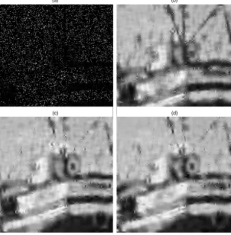
HereΩcorresponds to a Gaussian blur kernel with variance1.2.nis a white Gaussian noise with variance0.1. The resulting output SNR is14.90. The restored images are displayed on Fig. 2,λis such that the empirical variance of the residual is close to0.1(known as the Morozov’s discrepancy principle [17]).
(a) (b)
(c) (d)
Fig. 2. (a) degraded image (b) Soft (SNR = 20 dB). (c) NNG (SNR = 19.3 dB). (d) Hard (SNR = 19.6 dB).
On these experiments, one can see that the performances of all the thresholding operators are sensibly equivalent with a slight ad-vantage for the Soft-Thresholding. SCAD and Firm obtain similar results (not shown here).
4.2. Image inpainting
HereΩcorresponds to a mask of random pixel locations. The re-sulting image has90%missing pixels, with no additional noise. The restored images are displayed on Fig. 3, forλ→0. The given SNR are computed on the missing pixels only.
(a) (b)
(c) (d)
Fig. 3. (a) Degraded Image (b) Soft (SNR = 12.9 dB). (c) NNG (SNR = 14.6 dB). (d) Hard (SNR = 14.3 dB).
For this problem, the performances are inverted compared to the previous one: NNG and Hard-Thresholding give the bests SNR, while Soft gives the less satisfactory reconstruction. SCAD and Firm obtain similar results than NNG (not shown here).
5. DISCUSSION AND CONCLUSION
The results obtained to the previous toy problem confirm that good performances can be achieved with various thresholding rules, and the choice between Soft or Hard thresholding depends of the consid-ered problem. The choice of NNG (or SCAD, or Firm) thresholding rules appears to be a good compromise between this two operators. However, the results are not as impressive as in [18], where NNG was heuristically used inside ISTA for declipping audio signal, or in [18] where NNG was compared to other thresholding rules on au-dio denoising. In these two papers, NNG outperforms both Hard and Soft Thresholdings.
Still, the main objective of this article is to provide theoretical guarantee for using (relaxed)-ISTA with thresholding rules. One can notice that in [19], it was shown that an algorithm similar to relaxed-ISTA can be used in the context of nonconvex optimization. The main difference being that the algorithm studied in [19] involves several hyper-parameters when Alg. 1 has no parameter except the relaxation parameter.
The study made here can be extended straightforward to inde-pendant group shrinkage, following [13] which extends the approach of Antoniadis [3]. Generalization to data termfwhich is not Lips-chitz differentiable seems also possible, using an adaptive step size instead of the constant step size equal to1/L, following the analysis made by Tseng and Yun for block-coordinate descent in [20].
Finally, convergence analysis of ISTA with “thresholding” op-erators with overlap, as the windowed-group-Lasso [21] remains an open problem.
6. REFERENCES
[1] D. L. Donoho, “Nonlinear wavelet methods for recovery of signals, densities, and spectra from indirect and noisy data,” inProceedings of symposia in Applied Mathematics, vol. 47. Providence: American Mathematical Society, 1993, pp. 173– 205.
[2] S. G. Chang, B. Yu, and M. Vetterli, “Adaptive wavelet thresh-olding for image denoising and compression,”Image Process-ing, IEEE Transactions on, vol. 9, no. 9, pp. 1532–1546, 2000. [3] A. Antoniadis, “Wavelet methods in statistics: Some recent de-velopments and their applications,”Statistics Surveys, vol. 1, pp. 16–55, 2007.
[4] S. Chen, D. Donoho, and M. Saunders, “Atomic decomposi-tion by basis pursuit,”SIAM Journal on Scientific Computing, vol. 20, no. 1, pp. 33–61, 1998.
[5] R. Tibshirani, “Regression shrinkage and selection via the lasso,”Journal of the Royal Statistical Society Serie B, vol. 58, no. 1, pp. 267–288, 1996.
[6] M. Elad., “Why simple shrinkage is still relevant for redundant representations?” IEEE Transactions on Information Theory, vol. 52, no. 12, pp. 5559–5569, 2006.
[7] P. Combettes and V. Wajs, “Signal recovery by proximal forward-backward splitting,”Multiscale Modeling and Simu-lation, vol. 4, no. 4, pp. 1168–1200, Nov. 2005.
[8] A. Beck and M. Teboulle, “A fast iterative shrinkage-thresholding algorithm for linear inverse problems,” SIAM Journal on Imaging Sciences, vol. 2, no. 1, pp. 183–202, 2009. [9] M. A. Figueiredo, R. D. Nowak, and S. J. Wright, “Gradi-ent projection for sparse reconstruction: Application to com-pressed sensing and other inverse problems,”Selected Topics in Signal Processing, IEEE Journal of, vol. 1, no. 4, pp. 586– 597, 2007.
[10] M. E. D. T. Blumensath, “Iterative thresholding for sparse ap-proximations,”The Journal of Fourier Analysis and Applica-tions, vol. 14, no. 5, pp. 629–654, 2008.
[11] J. Bolte, H. Attouch, and B. Svaiter, “Convergence of descent methods for semi-algebraic and tame problems: proximal al-gorithms, forward-backward splitting, and regularized gauss-seidel method,”Mathematical Programming, vol. 137, no. 1–2, pp. 91–129, 2013.
[12] Y. She, “Thresholding-based iterative selection procedures for model selection and shrinkage,”Electronic Journal of Statis-tics, vol. 3, 2009.
[13] ——, “An iterative algorithm for fitting nonconvex penalized generalized linear models with grouped predictors,” Computa-tional Statistics & Data Analysis, vol. 56, no. 10, pp. 2976– 2990, 2012.
[14] P. Gong, C. Zhang, Z. Lu, J. Z. Huang, and J. Ye, “A gen-eral iterative shrinkage and thresholding algorithm for non-convex regularized optimization problems,” Journal of Ma-chine Learning Research, vol. 28, no. 2, pp. 37–45, 2013. [15] A. Colesanti and D. Hug, “Hessian measures of semi-convex
functions and applications to support measures of convex bod-ies,”manuscripta mathematica, vol. 101, no. 2, pp. 209–238, 2000.
[16] M. Bazaraa and C. Shetty,Nonlinear Programming: Theory and Algorithms, Wiley ed., New York, 1979.
[17] V. A. Morozov, “On the solution of functional equations by the method of regularization,”Soviet Math. Dokl., vol. 7, pp. 414–417, 1966.
[18] K. Siedenburg, M. D¨orfler, and M. Kowalski, “Audio declip-ping with social sparsity,”Preprint, 2013.
[19] P. Ochs, Y. Chen, T. Brox, and T. Pock, “ipiano: Inertial prox-imal algorithm for non-convex optimization,”Preprint, 2013. [20] P. Tseng and S. Yun, “A coordinate gradient descent method for
nonsmooth separable minimization,”Math. Prog. B, vol. 117, pp. 387–423, 2009.
[21] M. Kowalski, K. Siedenburg, and M. D¨orfler, “Social sparsity! neighborhood systems enrich structured shrinkage operators,”
IEEE transactions on signal processing, vol. 61, no. 10, pp. 2498–2511, 2013.