Evaluation and Comparison of Dynamic Treatment Regimes: Methods and Challenges.

(1)

Evaluation and Comparison of Dynamic Treatment

Regimes: Methods and Challenges

by Xi Lu

A dissertation submitted in partial fulfillment of the requirements for the degree of

Doctor of Philosophy (Statistics)

in the University of Michigan 2015

Doctoral Committee:

Professor Susan A. Murphy, Chair

Research Assistant Professor Daniel Almirall Assistant Professor Lu Wang

(2)

©Xi Lu 2015

(3)

Dedication To my parents

(4)

LIST OF FIGURES

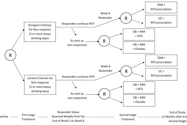
2.1 ExTENd SMART design for the treatment of alcohol dependence. “R” stands

for (re-)randomization. TDM = Telephone Disease Management, UC = Usual Care, NTX = Naltrexone, CBI = Combined Behavioral Intervention, MM =

Medical Management. . . 11

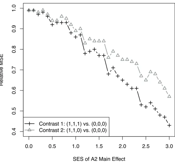
2.2 Relative mean squared error of the two assisted estimators, as a function of the

SES ofA2main effect in the generative model. . . 42

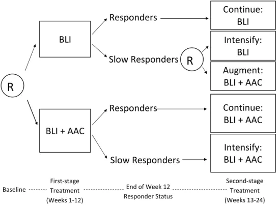
3.1 A SMART study for developing a DTR for children with autism who are

min-imally verbal. R = randomization. BLI = behavioral language intervention.

AAC = augmentative or alternative communication approach. . . 47

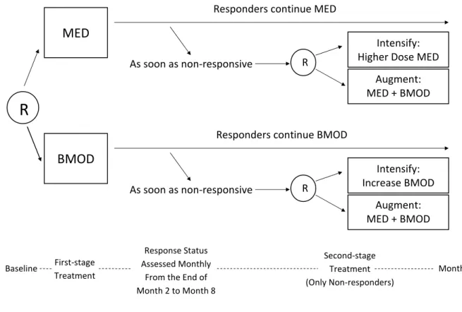
3.2 A SMART study for developing a DTR for children with attention deficit/hyperactivity

disorder. R = randomization. MED = medication. BMOD = behavioral

modi-fication. . . 49

3.3 A SMART study for developing a DTR for adults with alcohol dependence. R

= randomization. NTX = Naltrexone. TDM = telephone disease management. UC = usual care. CBI = combined behavioral interventions. MM = medical

management. . . 50

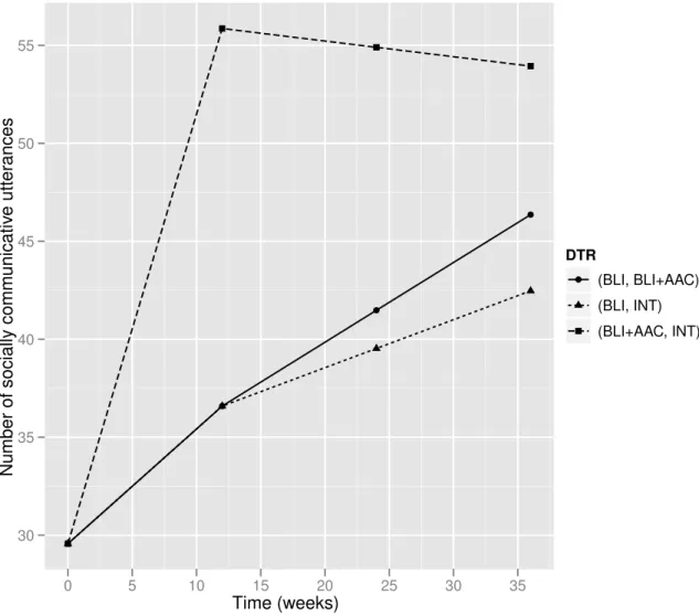
3.4 Estimated mean trajectories under the embedded DTRs of the autism SMART. 64

3.5 Estimated mean trajectories under the embedded DTRs of the ADHD SMART. 67

3.6 Estimated mean trajectories under the embedded DTRs of the ExTENd SMART.

a1 (the definition for non-response) and a2 (stage two treatment regime) jointly

specify the eight embedded DTRs. . . 69

3.7 Exploratory plot of ADHD SMART: empirical mean of the repeated-measures

outcome under each embedded DTR, at each time point. . . 81

3.8 True mean trajectories of the repeated measures under the embedded DTRs,

under four data-generative models corresponding to effect size (of the contrast

(7)

LIST OF TABLES

2.1 Simulation 1: Statistical properties of the assisted estimators of the contrast

between values of policies (1,1,1) and (0,0,0). Oracle = contrast estimator

based onVˆmd(d; ˆβ)with the true optimalmd. Assist = contrast estimator based

onVˆmˆd(d; ˆβ)with a working estimate of the optimalmd. Assist (md = 0) =

contrast estimator based on Vˆ0(d; ˆβ). The displayed numbers for confidence

interval coverage are the coverage proportion × 100. An Asterisk indicates

that the MSE of Oracle or Assist (md = 0) is significantly different from MSE

of Assist (at0.05level). . . 22

2.2 Simulation 2: Comparison between the marginal-mean-model-based

estima-tors and the assisted estimaestima-tors, with respect to the performance in estimating

the policy contrasts, withN = 100. MM = Marginal-mean-model-based

esti-mator. Assist1 = Assisted estimator with correctly specified SNMM. Assist2 =

Assisted estimator with mis-specified SNMM that excludesX11, X21, RX21.

Assist3 = Assisted estimator with mis-specified SNMM that excludes all the covariates interacting with treatments. Bias significantly different from 0, and coverage proportion significantly different from 95%, are marked with an

as-terisk. Relative MSE is calculated as the ratio of MSE with that of MM. . . . 24

2.3 Simulation 2: Comparison between the marginal-mean-model-based

estima-tors and the assisted estimaestima-tors, with respect to the performance in estimating

the policy contrasts, withN = 250. MM = Marginal-mean-model-based

esti-mator. Assist1 = Assisted estimator with correctly specified SNMM. Assist2 =

Assisted estimator with mis-specified SNMM that excludesX11, X21, RX21.

Assist3 = Assisted estimator with mis-specified SNMM that excludes all the covariates interacting with treatments. Bias significantly different from 0, and coverage proportion significantly different from 95%, are marked with an

as-terisk. Relative MSE is calculated as the ratio of MSE with that of MM. . . 25

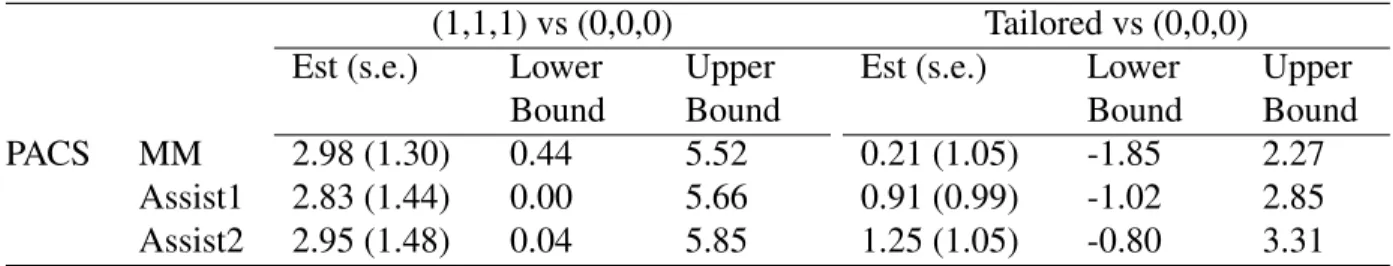
2.4 Illustrative data analysis results with the ExTENd data. Evaluate the policy

contrasts of both the policy (1, 1, 1) and the proposed tailored policy, in re-lation to the policy (0, 0, 0), with respect to PACS. MM = Marginal-mean-model-based estimator. Assist1 = Assisted estimator with a parsimonious

(8)

2.5 Simulation 1*: Statistical properties of the assisted estimators of the contrast

between values of policies (1,1,1) and (0,0,0), whenβˆdoes not belong toB.

Assist = contrast estimator based onVˆmˆd(d; ˆβ)with a working estimate of the

optimalmd. Assist (md = 0) = contrast estimator based onVˆ0(d; ˆβ). The

dis-played numbers for confidence interval coverage are the coverage proportion

×100. An Asterisk indicates that the MSE of Assist (md= 0) is significantly

different from MSE of Assist (at0.05level).. . . 41

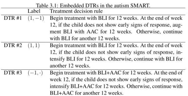
3.1 Embedded DTRs in the autism SMART. . . 48

3.2 Design features of ExTENd study and their implications on the

repeated-measures modeling.. . . 57

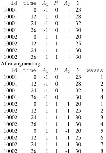
3.3 Example of a chunk of data before and after augmenting. The augmented data

set is ready to be analyzed bygeeglmingeepack. . . 63

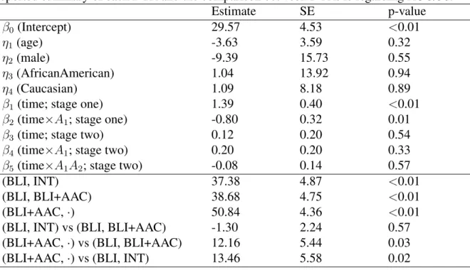
3.4 An analysis of the repeated-measures outcome from the autism SMART. The

reported summary of each DTR and the comparison between DTRs is

regard-ing AUC/36. . . 65

3.5 An analysis of the repeated-measures outcome from the ADHD SMART. The

reported summary of each DTR and the comparison between DTRs is

regard-ing AUC/7. . . 66

3.6 An analysis of the repeated-measures outcome from the ExTENd SMART.

LNT=lenient non-response definition. STRGT=stringent non-response

defini-tion. NTX=naltrexone+CBI. PLC=placebo+CBI. . . 70

3.7 Bias and Relative MSE (in relation to model (a) that respects the design

fea-tures of a SMART) of estimates from the slope model and the quadratic model.

∆AU C₁ =the constrast in AUC between DTRs (1, 1) and (1, -1);∆AU C₂ =the

contrast in AUC between DTRs (-1,·) and (1, -1). Bias that significantly

dif-fers from zero is in bold. . . 72

3.8 Comparison between two implementations of the proposed estimator

(GEE-I uses an independent working correlation; GEE-exch uses an exchangeable

working correlation), concerning the estimation of two estimands: ∆AU C

1 =

the constrast in AUC between DTRs (1, 1) and (1, -1);∆AU C₂ =the contrast

in AUC between DTRs (-1,·) and (1, -1). . . 74

4.1 Coverage of confidence intervals constructed by plug-in sandwich estimators

(Plug-in) and sandwich estimators with small-sample bias correction (BC), for the variances of WR estimators, in four simulation scenarios where the

within-person correlation (ρ) amongL1, L2, Y varies. ∆1 = the mean difference

be-tween DTRs (1, 1) and (1, -1);∆2 = the mean difference between DTRs (-1,

(9)

ABSTRACT

Evaluation and Comparison of Dynamic Treatment Regimes: Methods and Challenges

by Xi Lu

Chair: Professor Susan A. Murphy

Dynamic treatment regimes (DTRs) are sequences of decision rules that link the patient history with treatment recommendations. Clinical scientists have become increasingly interested in the development of DTRs in various fields including substance abuse, mental health and cancer. The Sequential Multiple Assignment Randomized Trial (SMART) is a multi-stage trial design that explicitly targets the development of high-quality DTRs. In this dissertation, we develop statistical methodologies, which can be applied to SMART data, that either address novel research questions regarding the construction of a high-quality DTR, or exhibit better performance than existing statistical methods.

(10)

CHAPTER 1

Introduction

In many areas of health, treatment response is heterogeneous in which case clinicians will need to consider providing a sequence of treatments in order to obtain sufficient treatment response. Furthermore patients with chronic illnesses often require changes in treatment, that is, sequences of treatments, so as to maintain a good response. As a result clinical scientists have become increasingly interested in, and active in, the development of inter-ventions that are composed of treatment sequences [25] in various fields including alco-holism [48], substance abuse [18, 35], leukemia [75] and autism spectrum disorder [19]. The treatment sequences are adapted to the dynamics of the evolving illness. The idea is that the adaptation should accommodate treatment response heterogeneity so as to result in more efficacious and less burdensome/costly treatment. Treatment policies [33, 82, 83] – also called dynamic treatment regimes (DTRs) [51,56,57,58,64,41], adaptive treatment strategies [25, 27, 26, 40, 74, 75] or adaptive interventions [43, 44, 1] – operationalize the dynamic adaption via a sequence of decision rules, one for each stage in the treatment process; the decision rule inputs measurements of patients’ time-varying covariates and outputs recommended treatments.

The Sequential Multiple Assignment Randomized Trial (SMART; [25,40,9]), a multi-stage trial design, was developed explicitly for the development of high-quality DTRs. Specifically, data from SMART design is useful in addressing key research questions that inform the construction of a high-quality DTR. Each stage in a SMART corresponds to one of the critical decisions involved in the DTR. Each participant moves through the multiple stages and at each stage the participant is (re)randomized to one of several intervention op-tions. A variety of these trials have been conducted, with some of the earliest taking place in cancer research, for the purpose of developing medication algorithms for leukemia [75], or to develop adaptive treatments of prostate cancer [74]. A selection of SMART studies may be found athttp://methodology.psu.edu/ra/adap-inter/projects. Com-mon research questions regarding DTRs that can be addressed by analyzing SMART data include: (a) the comparison of different intervention options at each of multiple stages of

(11)

the intervention; (b) the comparison among a pre-determined set of DTRs (usually “em-bedded” in the design of a SMART, which we later explain in Chapter 3) in terms of an end-of-study primary outcome.

In the following chapters in this dissertation, we will develop statistical methodologies that either address novel research questions regarding the construction of a high-quality DTR, or exhibit better performance than existing methods/statistical procedures. The topics that are discussed in this dissertation will cover a variety of aspects in the analysis of data arising from SMARTs, or more generally, randomized clinical trials. It is worthwhile to note that there are also extensive works concerning the design of (multi-stage) randomized clinical trials, for the purpose of optimizing various objectives. Those topics are not in the scope of this dissertation.

The dissertation is organized as follows. In the remainder of Chapter 1, we review the literature of methodological works related to evaluating and optimizing DTRs. In Chapter 2, we develop an “assisted estimator” that can be used to compare the mean outcomes of a pair of competing DTRs. The term “assisted” refers to the fact that estimators from the Structural Nested Mean Model (SNMM), a parametric model for the causal effect of treat-ment at each time point, are used in the process of estimating the mean outcome. This novel estimator significantly improves efficiency compared to the existing inverse-probability-of-treatment-weighted type of methods, by imposing parametric modeling assumptions on the components of the data distribution that are easily interpretable. Additionally, based on Robins’ G-estimators for the SNMM, we present an easy-to-implement least-squares esti-mator for the parameters in the SNMM.

In Chapter 3, we focus on the comparison of a pre-determined set of DTRs, in terms of a repeated-measures outcome that spans across multiple treatment stages. Modeling the marginal mean trajectories of a repeated-measures outcome arising from a SMART presents challenges, because traditional longitudinal models used for randomized clinical trials do not take into account the unique design features of SMART. In this chapter, we fill in this gap by discussing modeling considerations for various forms of SMART de-signs, emphasizing the importance of considering the timing of the repeated measures in relation to the treatment stages in a SMART. For illustration, we present three case studies with increasing level of complexity, in autism, child attention deficit hyperactivity disorder (ADHD), and adult alcoholism. The weighted-and-replicated estimators, which were orig-inally proposed for comparing DTRs in terms of an end-of-study outcome, are generalized to estimate the parameters in our repeated-measures model.

In Chapter 4, we concentrate on one particular aspect of the weighted-and-replicated (WR) estimators, namely the performance of the WR estimators on data sets with small

(12)

sample sizes. More specifically, in some numerical studies we found that the sandwich estimator for the variance of WR estimators derived from the standard Taylor series argu-ments does not provide confidence intervals that have good coverage, when the sample size is sufficiently small. The same phenomenon has been discovered in the GEE literature; intuitively, this happens because using the estimated parameters as a surrogate for the true unknown values of the parameters in general tend to “underestimate the variance of the true errors”. Based on [34] in the GEE literature, we propose a small-sample adjusted estimator for the variance of WR estimators. The adjustment is developed for the WR estimators with both known weights (due to the SMART design) and estimated weights.

In Chapter 5, we consider a novel research question regarding the search for the optimal decision rule. Primarily the goal is to identify the optimal policy, i.e., the one that yields the highest mean of an outcome variable, within a pre-specified class of parametrized poli-cies. On top of this goal, we are interested in understanding the usefulness of a particular variable in decision making, i.e., whether using this variable in addition to all the other variables in the specified policy form to construct a policy would remarkably increase the optimal achievable policy value. It turns out that estimating the optimal policy by sim-ply searching for the policy associated to the highest (non-parametrically) estimated policy value does not answer the second part of our research question, due to some interesting ill-posedness issues. In this chapter some preliminary endeavor is made towards this research question. We propose a regularized estimator for the optimal policy, with two components of regularization motivated by two issues of the original unregularized estimator.

1.1 Review of Existing Work on Dynamic Treatment Regime

Methodologies

Here we give a brief review of the literature on DTRs, mostly using data arising from an experiment study such as SMART.

A vast literature is available concerning the estimation of the optimal DTR based on data collected from both SMARTs and observational studies. A DTR is considered to be optimal if it yields the highest value of mean outcome when the entire population re-ceive treatment sequences that are specified by this DTR. Q-learning [72, 42, 69, 37] has been the most well studied methodology in this direction. A backward induction proce-dure mimicking dynamic programming is implemented, estimating the Q-function at each time point, which is the conditional mean of the primary outcome given certain values of current history of covariates and treatments, assuming that the optimal treatment is always

(13)

assigned in each of subsequent stages. The optimal DTR can then be estimated to consist of decision rules that recommend the treatment that maximizes the estimated Q-function at each stage. However, unbiased estimates and valid inference about the estimated opti-mal DTR can be difficult, because the “max” operator used in the Q-learning procedure can cause non-regularity. Some variations of Q-learning have been proposed, including the use of thresholding [8, 38] and the combination with LASSO [71]. There are also works that aim to directly draw valid inference from Q-learning based on bootstrap orm-out-of-n

bootstrap techniques [23,7].

On the other hand, the optimality, or good performance, of the estimated optimal DTR relies severely on the correct model specification of the Q-functions. More specifically, both the main effects of the covariates and the treatment interaction effects in each of the Q-functions have to be correctly specified to guarantee the optimality of the derived optimal DTR. This is a rather strong modeling assumption; mis-specification of the Q-functions may potentially lead to low mean value of the estimated optimal DTR. Advantage learning (A-learning; [39, 64]) is an alternative approach to estimating the optimal DTR. Unlike Q-learning, in A-learning only the part of outcome regression model that represents the contrasts among the treatments is parametrically modeled; this makes A-learning in general more robust than Q-learning to model mis-specification.

Another line of research that targets the estimation of the optimal DTR is the statisti-cal learning based methods developed by [89] and [90]; the former focuses on one time point and the latter extends the methodology for single time point to sequential treatments. The approaches proposed in these works cast the optimization of the value under the DTRs as weighted classification problems, where weights depend on the outcomes; as a conse-quence, existing machine learning algorithms can be directly applied to achieve the search for the optimal DTR. In particular, in these works the authors adopt the support vector machine (SVM) algorithm to relax the weighted classification problem; therefore, the the-oretical properties of the proposed methods naturally follow from the established theory of SVM.

Marginal mean model [41] is a model for the marginal mean of a primary outcome un-der a DTR, conditional on some baseline covariates. This methodology is essentially non-parametric in that it does not make non-parametric assumptions on the relationship between time-varying covariates and the outcome; consistency only relies on correct specification of the treatment assignment probability in the observed data, which helps to connect the mean in the hypothetical population where all individuals follow the specified DTR, to a weighted mean in the observed population. Such a model is estimated by a doubly robust inverse probability weighted estimator that contains some working models for a series of

(14)

conditional means to provide additional guarantee of robustness and potential efficiency improvement. Since the treatment assignment probability is known in SMARTs, the esti-mator based on the marginal mean model can easily be consistent. [87] provides another perspective of the estimator for marginal mean model that arises from coarsening of the sequential data, and has some insights about how the users might obtain reasonably good working estimates for the nuisance functions.

G-computation estimators [51] are another class of estimators that can be used to es-timate the marginal mean of the outcome under a DTR. This class of estimators is based on the representation of the marginal mean with conditional mean of the outcome given time-varying covariates, and the conditional distribution of the time-varying covariates. In the G-computation estimator, these conditional means and conditional distributions are re-placed by their estimates, respectively. This approach is conceptually intuitive; however, it requires correct model specification of many components in the data, which is particularly difficult when the covariates are of high dimension.

Marginal Structural Models (MSMs; [55], [63]) are a class of methods that were origi-nally proposed to model the causal effect of time-varying treatment as a function of base-line prognostic factors. MSMs can be readily applied to handle various types of primary outcomes. Later the MSM methodology was extended to investigate the causal effect of DTRs conditional on baseline prognostic factors [47, 78, 50, 3, 46]. This is achieved by modeling the mean of potential outcomes associated with each of the DTRs in the class of DTRs of interest. By nature of the MSM methodology, the model adopted in MSM needs to be chosen according to the class of DTRs under study. Doubly robust inverse probability weighted estimating equation can be used to estimate such models. Then the optimal DTR among the specified class of DTRs can be readily estimated by identifying the optimizer of the estimated values of the DTRs.

Targeted maximum likelihood estimation (TMLE; [77,6]) is another estimation proce-dure that can be taken to estimate a pre-specified parameter of the distribution of the ob-served data, such as the mean of an end-of-study outcome. The TMLE procedure targets a pre-specified estimand; more specifically, the procedure estimates the likelihood functions in a way that matches the efficient influence curve of the targeted parameter. The estimated likelihood functions are later used to construct the estimator for the targeted parameter via the G-computation formula. A TMLE is a substitution estimator, i.e., an estimator that can be conceptualized by replacing the unknown true underlying distribution with a particularly estimated distribution, in the defining formula of the estimand. Therefore it enjoys advan-tages that are specific to substitution estimators (e.g., the values of the estimator always lie in the reasonable range).

(15)

Methodological work that targets other types of outcomes is also available. Survival outcome (i.e., time to event outcome) is a particular type of outcome that usually requires special methodologies, and there have been a series of works about the comparison of DTRs regarding a survival outcome. [10] and [29] present weighted log-rank test statistic to compare a pair of DTRs that do not share observations (i.e., no participant can have treatment sequence that is consistent with these two DTRs at the same time). [21] develop weighted log-rank test statistic that can compare any pair of competing DTRs.

[85] proposes Bayesian inference methodology for the estimation and inference about DTRs. Under the Bayesian framework, potential outcomes under all possible treatment sequences are conceptualized as unknown parameters, and therefore posterior predictive distribution can be formed for the potential outcomes to facilitate estimation and inference about static and dynamic regimes. Moreover, the Bayesian approach naturally offers the po-tential to pool information across treatment paths and individuals in the same group/cluster.

(16)

CHAPTER 2

Comparing Treatment Policies with Assistance

from the Structural Nested Mean Model

2.1 Introduction

In many health domains, a treatment sequence that is adapted to patients’ evolving char-acteristics and past treatment history is needed. This is because the response to the same treatment/intervention can vary among patients with different baseline characteristics and time-varying health status. Moreover, a treatment that is associated with short-term success may not be preferable for controlling the disorder in the long term. One way to operational-ize the adaptation of the sequence of treatment to patients’ evolving status over time is via the treatment policies, which compose of a sequence of decision rules, one for each critical decision time point in the treatment process. At each critical decision time point (i.e., at each treatment stage), the decision rule takes the measurements of patients’ time-varying covariates as input, and determines the recommended treatments/interventions.

Often scientists construct treatment policies that represent competing approaches to managing an illness. For example in the treatment of attention deficit hyperactivity disor-der (ADHD), the American Psychological Association recommends starting with behav-ioral treatment and moving to a medication only if the behavbehav-ioral treatment is not effec-tive [4], whereas the American Academy of Child and Adolescent Psychiatry recommends starting with medication [49]. Or one treatment policy might represent a least intensive or least costly version, whereas another treatment policy may represent a most intensive, most costly version. For example, the Extending Treatment Effectiveness of Naltrexone (Ex-TENd) trial of alcohol dependence treatments (PI: Oslin; [48]) involves multiple treatment policies, of which one is the most intensive and another is the least intensive.

In this chapter, we develop and discuss statistical methodologies for the evaluation of a treatment policy and the comparison between two competing treatment policies, regarding the mean of a pre-specified primary outcome variable, that is either measured at the end

(17)

of the study, or an outcome variable calculated from the variables measured during the study. Some other endpoints for the comparison/evaluation of treatment policies might be possible. In particular, in the next chapter, we discuss the comparison among treatment policies regarding the mean trajectories of a repeated-measures outcome, the measurement of which spans through multiple treatment stages in a study.

A common approach to comparing the mean outcomes of two competing treatment policies, is to use a non-parametric estimation procedure that involves inverse-probability-weights (IPW), such as those described in [41] and [87]. These estimators are non-parametric in the sense that they do not require nor take advantage of models that relate baseline or time-varying covariates with the outcome. Robins and colleagues [54, 46] generalized the [41] methods to consider multiple treatment policies.

In this chapter, we develop an alternative approach for contrasting two treatment poli-cies. This approach combines the non-parametric IPW estimators with a model-based ap-proach based on Robins’ Structural Nested Mean Model [52]. In the Structural Nested Mean Model, intermediate treatment effect functions, also called “treatment blips,” are parametrically modeled. The intermediate treatment effects isolate the causal effect of treatment at each time point, conditional on baseline and time-varying covariate history up to that time point. We call the resulting estimator, an “assisted” estimator to convey that the model-based approach is intended to assist the non-parametric estimator in estimating the mean outcomes of competing treatment policies.

In this chapter we first focus on the comparison of two-stage treatment policies. Most sequentially randomized trials, also known as Sequential Multiple Assignment Random-ized Trials (SMART) [24, 40], concern two stages of treatment. In particular, ExTENd is a two-stage SMART. Towards the end of this chapter we will briefly discuss the exten-sion of the proposed methodology to the scenario of more than two treatment stages. In Section 2.2, we formulate the estimand in a precise manner. In this section we provide a class of assisted estimators for the mean outcome based on data from a SMART; theo-retical properties of the estimators are also provided. In Section 2.3, we briefly introduce how these estimators can be used to compare a pair of treatment policies and make infer-ence. Simulation studies, in Section 2.4, are used to investigate different aspects of the methodology, including the performance of the proposed estimator under various levels of mis-specifying treatment effects. In Section2.5, the methodology is illustrated by an anal-ysis of the ExTENd data. In Section 2.6, we briefly introduce some ideas about how the proposed estimator can be extended to apply to three-stage problems. Finally, a discussion of the paper, including ideas for future work, is presented in Section 2.7. Proofs of the theorems and lemmas are relegated to the appendix.

(18)

2.2 Assisted Estimator for Policy Value

A two-stage treatment policy consists of two decision rules, d = (d1, d2). Each deci-sion rule inputs available patient information at the current stage and outputs a treat-ment recommendation. Denote the outcome by Y (Y may be observed after the study or may be a function of the data collected during the study). The value of a policy is the expectation of Y that would result if the treatments were selected using the treat-ment policy d. A useful way to define the value of a policy is via the potential out-come framework [45, 68]. For each variable and each treatment sequence, we concep-tualize a “potential outcome” that would have been observed under that treatment se-quence. UsingXj to denote observations available prior to thej-th decision and usingX3 to denote observations available after the second-stage treatment, the potential outcomes are {X1, X2(a1), X3(a1, a2); for all possible sequences of treatments(a1, a2)}. Here the outcome Y(a1, a2) is a known function of {X1, X2(a1), X3(a1, a2)}. The value of the policy, d, is given by Vd = E

Y(a1, a2)|a2=d2(H2(a1)),a1=d1(H1)

where H1 = X1 and

H2(a1) = (X1, a1, X2(a1))are the potential outcome history vectors prior to the treatments at stage one and stage two.

The value of a treatment policy d, can also be written as a function of the intermedi-ate treatment effects or “treatment blip functions,” from Robins’ Structural Nested Mean Model [52]. We deviate briefly to define these intermediate treatment effects. Correspond-ing to the two stages of treatment, there are two intermediate treatment effects given by

µ2(h2, a2) = E[Y(a1, a2)|H2(a1) = h2] −E[Y(a1,0)|H2(a1) = h2] and µ1(h1, a1) =

E[Y(a1,0)|H1 = h1]−E[Y(0,0)|H1 = h1], whereat = 0is the coding for a reference

treatment (e.g., control treatment). The intermediate treatment effect, µ2, quantifies the effect of treatment a2 relative to the reference treatment at stage two on the mean of Y, among individuals with history h2. The intermediate treatment effect, µ1, quantifies the effect of treatmenta1 relative to the stage one reference treatment, if always followed by the reference treatment at stage two, on the mean ofY, among individuals with historyh1 at stage one. In addition to this type of treatment blip functions, there are other types of blips, such as the optimal-blip-to-zero functions for A-learning [39] and regime-specific SNMMs [64].

Consider randomized treatments, denoted by capitalized letters,A1, A2, where the con-ditional distribution of A1 given H1 = h1 is denoted byp1(·|h1)and the conditional dis-tribution of A2 given H2(A1) = h2 is denoted by p2(·|h2). Throughout this chapter we implicitly make all required measurability assumptions as well as existence of regular con-ditional densities. We have the following lemma.

(19)

Lemma 2.2.1. Assume that (i) max{E|Y(a1, a2)|, E|µ1(H1, a1)|, E|µ2(H2(a1), a2)|} <

∞ for any treatment sequence (a1, a2) and (ii) for some δ > 0, p1(a1|h1) ≥ δ a.s. for (h1, a1), then Vd = E h Y(A1, A2)−µ2(H2(A1), A2)−µ1(H1, A1) +µ1(H1, d1(H1)) +µ2(H2(a1), d2(H2(a1)))|a1=d1(H1) i = EhY(A1, A2)−µ2(H2(A1), A2)−µ1(H1, A1) +µ1(H1, d1(H1)) +I{A1 =d1(H1)} p1(A1|H1) µ2(H2(A1), d2(H2(A1))) i . (2.1) This representation of the value,Vd, will form the basis for our method. The intuition

behind this representation is that the potential outcome ofY under treatment policydcan be constructed or recovered from the potential outcome associated with the treatment sequence (A1, A2), by subtracting the intermediate treatment effects due to the sequence (A1, A2) and then adding in the intermediate treatment effects due to the policy d. The fraction involving the randomization probability in the last term (2.1) is used to account for the fact that the intermediate treatment effect of the second stage treatment under policyddepends onH2(a1)|a1=d1(H1)(the covariate history that would occur if the first stage treatment were

assigned according to policyd); that is, this fraction adjusts for the fact thatH2(A1)is not always equal toH2(d1(H1)).

2.2.1 The Data and the Estimation Method

The observed data on each participant in a two-stage SMART is {X1, A1, X2, A2, X3} whereXt denotes covariates observed prior to thet-th stage andAtdenotes thet-th stage

randomized treatment. LetH2 = (X1, A1, X2)andH1 = X1. The randomization proba-bility for an individual’s treatment may be a function of the individual’s observed data (say

P[At = a|Ht] = pt(a|Ht)). For example, in ExTENd (see Figure2.1), participants were

initially randomized uniformly to one of two criteria for early non-response to Naltrexone: the stringent definition (two or more heavy drinking days) or the lenient definition (five or more heavy drinking days). A heavy drinking day is defined as a day with more than five standard drinks for males or more than four standard drinks for females. Participants were assessed weekly for non-response; as soon as a participant met the non-response criterion, he/she was re-randomized to either switch to combined behavioral interventions (CBI) or to a combination of CBI and Naltrexone. If the participant did not meet his/her assigned

(20)

non-response criterion by the end of two months, then the participant was re-randomized to one of two relapse prevention options: usual care (UC) or telephone disease management (TDM). Thus non-responding participants had probability 0 of being assigned a relapse prevention option whereas responding participants had probability 0 of being assigned CBI or the combination of CBI and Naltrexone.

Stringent Criterion for Non-response (2 or more heavy drinking days) Responders continue NTX As soon as non-responsive TDM + NTX prescription UC + NTX prescription CBI + MM + NTX CBI + MM + Placebo R Baseline First-stage Treatment Responder Status Assessed Weekly from the

End of Week 2 to Week 8

Second-stage Treatment

End of Study (2 Months after Entry to

Second Stage) Week 8

Responder _R

R

Lenient Criterion for Non-response (5 or more heavy drinking days) Responders continue NTX As soon as non-responsive TDM + NTX prescription UC + NTX prescription CBI + MM + NTX CBI + MM + Placebo R Week 8 Responder _R

Figure 2.1: ExTENd SMART design for the treatment of alcohol dependence. “R” stands for (re-)randomization. TDM = Telephone Disease Management, UC = Usual Care, NTX = Naltrexone, CBI = Combined Behavioral Intervention, MM = Medical Management

Denote the primary outcome by Y (we assume a higher value is more favorable; in ExTENdY might be percent days abstinent or a mental health score). To express the inter-mediate effects and the value (2.1) in terms of the observed data, we relate the observed data to the potential outcomes. We assume [66,53,50], (A1) Consistency:X2 =X2(A1), X3 =

X3(A1, A2), Y =Y(A1, A2)and (A2) Sequential Randomization:A1 is independent of all potential outcomes given observedX1;A2 is independent of all potential outcomes given observed(X1, A1, X2). The consistency assumption states that the observed covariates are

(21)

identical to the potential outcomes of the covariates evaluated at the observed treatment se-quence. In particular this assumption implies that each subject’s outcomes are uninfluenced by other subjects’ assigned treatments. This assumption may be violated if for example, treatment is provided in a group setting (group counseling). The sequential randomization assumption is valid in the setting of SMART trials because the treatment is randomized.

The intermediate treatment effects and the value,Vd, can be expressed in terms of the

observed data as follows.

Lemma 2.2.2. Assume A1 and A2 and (i)max{E|Y|, E|µ1(H1, a1)|, E|µ2(H2, a2)|}<∞

for any treatment sequence(a1, a2)and (ii) for someδ >0,p1(a1|h1)≥δa.s. for(h1, a1),

then (a) µ2(h2, a2) =E[Y|H2 =h2, A2 =a2]−E[Y|H2 =h2, A2 = 0], (b) µ1(h1, a1) = E[E[Y|H2, A2 = 0]|H1 = h1, A1 = a1]−E[E[Y|H2, A2 = 0]|H1 = h1, A1 = 0]and (c) Vd=E h Y−µ2(H2, A2)−µ1(H1, A1)+µ1(H1, d1(H1))+ I{A1=d1(H1)} p1(A1|H1) µ2(H2, d2(H2)) i .

Suppose the intermediate treatment effects are known up to a finite-dimensional pa-rameter: µ1(h1, a1) = µ1(h1, a1;β1), µ2(h2, a2) = µ2(h2, a2;β2). [52] provides a class of “g-estimators” for the parameters, β = (β1, β2). Each member in the class corresponds to a different choice of model for each of several nuisance functions; consistency of the g-estimators does not require correct models for the nuisance functions (see [52] for a de-tailed discussion). Furthermore this class of estimators does not require knowledge of the treatment policy, d. Thusβ can be estimated and then used to form the estimators of the values of a variety of treatment policies. In the next section, we review the class of g-estimators. Each estimator in this class is consistent for the true value β0 = (β10, β20)of

β, and is asymptotically normally distributed (assuming a correctly specified SNMM and some finite moment conditions). Throughout the chapter we implicitly assume consistency and asymptotic normality ofβˆ.

Then, given the results of Lemma2.2.2and estimators, βˆ, a natural assisted estimator of the value of the policyd,Vdis:

ˆ V0(d; ˆβ) = Pn h Y −µ2(H2, A2; ˆβ2)−µ1(H1, A1; ˆβ1) +µ1(H1, d1(H1); ˆβ1) (2.2) +I{A1 =d1(H1)} p1(A1|H1) µ2(H2, d2(H2); ˆβ2) i ,

(22)

where _Pnf(X1, A1, X2, A2, X3) denotes a sample average. This estimator belongs to a class of assisted estimators, given by

ˆ Vm(d; ˆβ) =Pn h Y −µ2(H2, A2; ˆβ2)−µ1(H1, A1; ˆβ1) +µ1(H1, d1(H1); ˆβ1) (2.3) +I{A1 =d1(H1)} p1(A1|H1) n µ2(H2, d2(H2); ˆβ2)−m(H1, A1) o +m(H1, d1(H1)) i ,

indexed by the function m(h1, a1). Note the former assisted estimator, Vˆ0(d; ˆβ), corre-sponds to settingm(h1, a1)≡0. We have the following lemma:

Lemma 2.2.3. Assume that the assumptions for Lemma2.2.2hold, then

(a) The estimating function in(2.3)is unbiased for any choice ofmthat satisfiesE|m(H1, a1)|<

∞for anya1.

(b) Assume (i)E|Y|2 _< _∞_{; (ii)}_µ_˙

1(h1, a1;β1) := _∂β∂₁µ1(h1, a1;β1) exists for allβ1, a.s.,

andµ˙2(h2, a2;β2) := _∂β∂₂µ2(h2, a2;β2)exists for allβ2, a.s.; and (iii) there exists some

a subclass B of g-estimators, the choice of m resulting in the lowest variance for

ˆ

Vm(d; ˆβ)satisfiesm(h1, d1(h1)) =E[µ2(H2, d2(H2))|H1 =h1, A1 =d1(h1)].

The subclass B corresponds to g-estimators for which a particular nuisance function is correctly modeled. This subclass is defined in Section 2.2.2 after a general review of g-estimators; in particular, in the simulation section we will first use an estimatorβˆbased on a correctly specified model for the nuisance function, thusβˆ∈B. We will also provide additional simulation results when using aβˆthat does not belong toB.

The lemma above provides a guide for the choice of m; in practicem(h1, a1)in (2.3) can be replaced by a working estimatormˆ(h1, a1) := m(h1, a1; ˆαm)ofE[µ2(H2, d2(H2))|H1 =

h1, A1 = a1], resulting inVˆmˆ(d; ˆβ). Next we provide consistency and asymptotic normal-ity results for the estimators of the value. We assume A1 and A2; in addition, we assume thatµ1(h1, a1;β1)andµ2(h2, a2;β2)are functions that correctly specify the SNMM, with true parameter valueβ0 = (β10, β20). In particular, Theorem2.2.4below implies that the assisted estimator is consistent regardless of the choice of functionm(indeed one can set

m≡0).

Theorem 2.2.4. Assume that the assumptions for Lemma2.2.3 hold; moreover, assume: (1) αˆm converges in probability to some limitα+m; (2) there exists some δ > 0 such that P

a1Esupkαm−α+mk≤δ|m(H1, a1;αm)|<∞; and (3)m˙(h1, a1;αm) :=

∂

∂αmm(h1, a1;αm)

(23)

Theorem 2.2.5. Assume that the assumptions for Theorem2.2.4hold; moreover, assume: (1) there exists someδ >0such thatP

a1Esupkαm−α+mk≤δ|m(H1, a1;αm)| 2₊_|_m_˙₍_H 1, a1;αm)|2 < ∞and (2)√n( ˆαm−α+m) =Op(1). Then √ nVˆmˆ(d; ˆβ)−Vd is asymptotically normal.

The asymptotic variance of the limiting normal distribution in Theorem 2.2.5 is pro-vided in the appendix. Recall that ifm(h1, a1;αm)is a correct model forE[µ2(H2, d2(H2))|H1 =

h1, A1 =a1], then this asymptotic variance achieves the lowest value among all choices of

m, provided thatβˆbelongs to the subclassB of g-estimators.

2.2.2 Estimators for SNMM

2.2.2.1 Review: Robins’ G-Estimators for SNMM

Here we give a brief review of Robins’ class of g-estimating equations [52] and the semi-parametric locally efficient g-estimator. Assume that the SNMM is correctly specified. A class of estimating equations which can be used to solve for consistent estimators forβ is:

Pn n r1(H1, A1) (Y −µ2(H2, A2;β2)−µ1(H1, A1;β1)−q1(H1)) +r2(H2, A2) (Y −µ2(H2, A2;β2)−q2(H2)) o = 0,

wherer1, r2 are arbitrary functions, both of the same dimension as the length of(β1T, β2T), that satisfyE[r1(H1, A1)|H1]≡0, E[r2(H2, A2)|H2]≡0;q1, q2are arbitrary functions.

Assume that V ar(Y −µ2(H2, A2)−µ1(H1, A1)|H1, A1) ≡ V ar(Y −µ2(H2, A2)−

µ1(H1, A1)|H1), which we will denote asσ12(H1), and thatV ar(Y−µ2(H2, A2)|H2, A2)≡

V ar(Y −µ2(H2, A2)|H2), which we will denote asσ22(H2). Robins providesr1, r2, q1, q2 functions that make the estimating equation semiparametric locally efficient; in particular the semiparametric locally efficient estimating equation is obtained by setting

q₁∗(h1) = E[Y −µ2(H2, A2;β20)−µ1(H1, A1;β10)|H1 =h1], q∗₂(h2) = E[Y −µ2(H2, A2;β20)|H2 =h2], r∗₁(h1, a1) =σ1−2(h1) ˙ µ1(h1, a1;β10)−E[ ˙µ1(H1, A1;β10)|H1 =h1] E[ ˙µ2(H2, A2;β20)|H1 =h1, A1 =a1]−E[ ˙µ2(H2, A2;β20)|H1 =h1] ! and r∗₂(h2, a2) =σ2−2(h2) 0 ˙ µ2(h2, a2;β20)−E[ ˙µ2(H2, A2;β20)|H2 =h2] ! .

(24)

Consider models forr1(·), r2(·), q1(·), q2(·), namelyr1(·;η), r2(·;η), q1(·;ξ), q2(·;ξ). If the parametric models specified forr1, r2, q1, q2 contain the truth (i.e., r∗1, r

∗ 2, q ∗ 1, q ∗ 2), the esti-mator forβis then semiparametric efficient.

Definition of B: The subclass B of estimators is defined as the collection of g-estimators in whichq1(h1;ξ)is a correctly specified model forq1∗(h1). In Lemma2.2.3, we show that the optimalmfunction in the assisted estimator can be identified ifβˆbelongs to this subclass. Note that the semiparametric efficient estimator belongs to this subclass.

2.2.2.2 Regression-Type Implementation of the G-Estimator

It turns out that for particular models of the nuisance functions (i.e., r1, r2, q1, q2) in the g-estimating equation, one can estimate both the nuisance functions and theβ’s simultane-ously via least-squares. We use this approach to estimate theβparameters in the interme-diate treatment effects in our simulations. We assume that the treatment effect functions are linear in the unknown parameters:µ1(h1, a1;β1) = φ1(h1, a1)Tβ1andµ2(h2, a2;β2) =

φ2(h2, a2)Tβ2, whereφtis some feature of(ht, at). The estimation is as follows:

1. First solve a linear regression of Y on (φ2(H2, A2)−E[φ2(H2, A2)|H2], M2), in which M2 is a summary of the history H2. Note that in the setting of a random-ized trial, the distribution of A2 is known; thus E[φ2(H2, A2)|H2] can be calcu-lated. Put βˆ2 equal to the vector of the estimated coefficients for φ2(H2, A2) −

E[φ2(H2, A2)|H2].

2. Second solve a linear regression ofY −φ2(H2, A2)Tβˆ2 on

(φ1(H1, A1)− E[φ1(H1, A1)|H1], M1), in which M1 is a summary of the history

H1. Again since the distribution of A1 is known, E[φ1(H1, A1)|H1] can be cal-culated. Put βˆ1 equal to the vector of the estimated coefficients for φ1(H1, A1)−

E[φ1(H1, A1)|H1]. ˆ

β obtained from this least-squares implementation is equivalent to a g-estimator with the following choice of nuisance functions:r1(H1, A1) = ˜φ1(H1, A1),r2(H2, A2) = ˜φ2(H2, A2),

q1(H1) = M1Tκ+1 −E[φ1(H1, A1)|H1]Tβ10, q2(H2) = M2Tκ+2 −E[φ2(H2, A2)|H2]Tβ20, where φ˜1 ≡ φ˜1(H1, A1) = φ1(H1, A1) − E[φ1(H1, A1)|H1] and φ˜2 ≡ φ˜2(H2, A2) =

φ2(H2, A2)−E[φ2(H2, A2)|H2];κ+1 andκ +

2 denote the probabilistic limits of the estimated coefficients of M1 and M2 in the least-squares procedure. In particular, this regression-type estimator is consistent with correctly specified SNMM. Note thatβˆobtained from this least-squares implementation belongs to the subclassB defined previously, provided that

MT

(25)

Each member of the class of g-estimators is consistent and asymptotically normal. In particular, the asymptotic distribution of √n( ˆβ −β0) is a multivariate normal with mean zero and var-covariance matrixB−1_Σ_B−1,T _where

B = E[ ˜φ1 ˜ φT 1] E[ ˜φ1φT2] 0 E[ ˜φ2φ˜T2] ! andΣ = E (Y −φT₂β20−φ˜T1β10−M1Tκ+1) ˜φT1,(Y −φ˜T2β20−M2Tκ+2) ˜φT2 T⊗2 , where

V⊗2 ₌_{V V}T_{. Plug-in estimates}_B_ˆ _and_Σ_ˆ _{can be obtained by replacing population}

expecta-tion inB andΣwith sample mean, and replacingβ, κby the estimates from the series of least squares.

Prior to this least-squares type estimator for the SNMM, [2] proposed a parametric two-stage estimator that can be implemented by linear regression. Consistency of the estimator therein requires correct model specification for both the intermediate treatment effects (i.e.,

µ1, µ2) and the nuisance functions associated to the time-varying error terms.

2.2.3 Existing Work Regarding the Evaluation of A Treatment Policy

Here we review the methodologies for the evaluation and comparison of treatment policies proposed by [41] and [87]. We present those methods in the two-stage scenario.

[41] introduces the marginal mean models for the estimation of a mean response to a treatment policy (called DTR there). For simplicity, we ignore the discussion there about the mean value of a treatment policy over interesting subpopulations (denoted byZin [41]), and only consider the estimation of the marginal mean value of a policy in the entire popu-lation. The estimator is based on the equality

Ed[Y] =Eobs Wd( ¯A2,X¯2)Y , whereWd(¯a2,x¯2) = ωd,1(a1, x1)ωd,2(¯a2,x¯2)andωd,1(a1, x1) = I{A1=d1(X1)} p1(A1|H1) , ωd,2(¯a2,x¯2) = I{A2=d2( ¯X2,A1)}

p2(A2|H2) ; Ed is the expectation in the population where all individuals follow the

treatment policydand Eobs is the expectation in the observed population. Thus the basic

IPW estimator based on the marginal mean model isVˆ =_Pn

Wd( ¯A2,X¯2)Y

.

There is a potential to improve the efficiency of this estimator by augmenting it (moti-vated by projecting the original estimating equation off the score functions for the treatment assignment probabilities, which are nuisance parameters for the estimation of policy value),

(26)

namely ˆ V( ˆαg) =Pn ωd,1ωd,2Y + (g1(X1, d1(X1); ˆαg)−ωd,1g1(X1, A1; ˆαg)) +ωd,1(g2( ¯X2, A1, d2( ¯X2, A1); ˆαg)−ωd,2g2( ¯X2,A¯2; ˆαg)) ,

in which g2(¯x2,¯a2;αg) is a model for g2(¯x2,a¯2) := Eobs[Y|X¯2 = ¯x2,A¯2 = ¯a2] and

g1(x1, a1;αg)is a model forg1(x1, a1) := Eobs[g2( ¯X2, A1, d2( ¯X2, A1))|X1 =x1, A1 =a1]. These estimators are in essence non-parametric estimators that are obtained by properly weighting the observations in the data that happen to have the entire treatment sequences consistent with the policy, d, of interest. Data from those who have treatments consistent with the policydonly until the first stage, or data from those with treatments inconsistent with the policydfrom the entry to study, are utilized to varying degrees in the augmented estimators, to potentially improve the efficiency.

[87] presents a robust augmented inverse probability weighted estimator for the values of a restricted class of treatment policies. In their paper the problem of policy value estima-tion is cast as one of monotone coarsening; however, with some calculaestima-tion one can show that the general class of estimators proposed in this paper is equivalent to the estimators arising from the marginal mean model in Murphy et al. (2001). Here we briefly present the equivalence in the case of a two-stage problem.

For each two-stage policy d = (d1, d2), conceptualize the complete data to be the po-tential outcomes associated with d: (X1, X2(d1), Y(d1, d2)). Then a coarsening variable

Cd can be defined for the complete data as below: If A1 6= d1(H1), then Cd = 1. If

A1 = d1(H1) and A2 6= d2(H2), then Cd = 2. If A1 = d1(H1) and A2 = d2(H2), then Cd = ∞. Then define the hazard functions for this coarsening variable Cd as

fol-lows (coarsening at random is assumed, and in the scenario of sequential randomized trials this assumption is naturally satisfied): λd,1(X1) = P r(Cd = 1|X1), and λd,2(X1, X2) =

P r(Cd= 2|Cd≥2, X1, X2). Then the class of estimators (indexed by the functionsL1(x1) andL2(x1, a1, x2)) proposed in Zhang et al. (2013) can be written as:

Pn I{Cd=∞} (1−λd,1)(1−λd,2) Y +I{Cd= 1} −λd,1 1−λd,1 L1(X1)+ I{Cd = 2} −λd,2I{Cd≥2} (1−λd,1)(1−λd,2) L2(X1, A1, X2) ,

in which λd,1 = λd,1(X1), λd,2 = λd,2(X1, X2). The consistency of any estimator in this class is guaranteed, regardless of the choices ofL1, L2.

(27)

settingL1(X1) =g1(X1, d1(X1))andL2(X1, A1, X2) =g2( ¯X2, A1, d2( ¯X2, A1)).

In the simulation section, we will compare the assisted estimators with the estimators arising from the marginal mean models. Note that the model specification for gt(·)does

not have an impact on the consistency of the estimatorVˆ( ˆαg). Suggested by [41], to

guar-antee that the models forgtare consistent with each other under the null, in the simulation

experiments we model gt as linear inx¯tand independent ofa¯t. In particular, we estimate

g2(X1, A1, X2, A1; ˆαg)by regressing Y on intercept andX¯2, then regress the fitted values on intercept andX1to obtaing1(X1, A1; ˆαg).

2.3 Comparison between Treatment Policies

Suppose we are interested in comparing treatment policiesd = (d1, d2)andd˜= ( ˜d1,d˜2). Then, given an estimatorβˆfor the intermediate treatment effects, we obtain the following consistent estimator for the contrast betweendandd˜, i.e.,V_d˜−Vd:

( ˆVmd˜( ˜d; ˆβ)− ˆ Vmd(d; ˆβ)) =Pn h µ1(H1,d˜1(H1); ˆβ1)−µ1(H1, d1(H1); ˆβ1) (2.4) + I{A1 = ˜d1(H1)} p1(A1|H1) n µ2(H2,d˜2(H2); ˆβ2)−m_d˜(H1, A1) o − I{A1 =d1(H1)} p1(A1|H1) n µ2(H2, d2(H2); ˆβ2)−md(H1, A1) o +m_d˜(H1,d˜1(H1))−md(H1, d1(H1)) i ,

where the function m(h1, a1) is now subscripted by the policy d, to reflect that a good choice of functionmvaries withd(see the following lemma). For ease of notation, define ∆d(h1, a1) = md(h1, a1)−E[µ2(H2, d2(H2))|H1 =h1, A1 =a1].

Lemma 2.3.1. Assume that the conditions for Lemma 2.2.3 are satisfied; in particular, assume thatβˆbelongs to the subclassB of g-estimators. Then the choice ofmd andm_d˜

resulting in the lowest asymptotic variance for√n( ˆVmd˜( ˜d; ˆβ)−

ˆ

Vmd(d; ˆβ)), among the class

of estimators in(2.4)withmdandm_d˜being arbitrary functions of(h1, a1), satisfy: (1) for

h1 such that d1(h1) 6= ˜d1(h1), ∆_d˜(h1,d˜1(h1)) = ∆d(h1, d1(h1)) = 0; (2) forh1 such that

d1(h1) = ˜d1(h1),∆_d˜(h1,d˜1(h1)) = ∆d(h1, d1(h1)).

Lemma2.3.1implies that, for the purpose of estimating the policy contrast, it is reason-able to replacemd(h1, a1)with a working estimatemd(h1, a1; ˆαm)ofE[µ2(H2, d2(H2))|H1 =

h1, A1 =a1]. Then we have the following lemma concerning the estimator of the contrast in (2.4) withmd(h1, a1)replaced bymd(h1, a1; ˆαm). We will also refer to this estimator as

(28)

an “assisted estimator”. This lemma assumes that md(h1, a1; ˆαm)is modeled via a linear

modelDT

mαm whereDm is a function of(H1, A1)andαmis estimated via least squares. Lemma 2.3.2. Assume that the conditions for Theorem2.2.4and2.2.5are satisfied; then

√

n ( ˆVmˆd˜( ˜d; ˆβ)−

ˆ

Vmˆd(d; ˆβ))−(Vd˜−Vd)

converges in distribution to a normal distribution with mean zero and var-covariance matrix,Σ∆. The plug-in estimatorΣˆ∆is a consistent

estimator ofΣ∆.

The formulae forΣ∆andΣˆ∆are provided in the appendix.

2.4 Simulation

All simulation experiments are based on generative models mimicking the ExTENd study. More specifically, the structure of the simulated data is: (X1, A1, X2, R, A2, Y). X1 is a 3-dimension baseline covariate simulating the distribution of{baseline percent days heavy drinking, baseline craving score, baseline mental composite score},A1is the binary indica-tor of the randomized non-response criterion,X2is a 2-dimension covariate simulating the distribution of{phase 1 duration, phase 1 percent days drinking},Ris the binary indicator of early response,A2 is the re-randomized binary treatment at the second stage. Y is a pri-mary outcome simulating the distribution of the end-of-study craving score (lower values are better). We will study various simulation scenarios that are all based on the following

Y:

Y =η0(X1)+A1(1, X1T)β1+η1(X1, A1, X2)+A2(1, X2T, A1, R, RX2T, RA1)β2+. (2.5) in which the terms involvingβ’s are the intermediate treatment effects andη0(·), η1(·)and

are other components in the distribution ofY that correspond to the main effect ofX1, the effect ofX2 conditional on(X1, A1)and the error term, respectively. We use estimates ofη0(·)andη1(·)that are by-products of estimating an SNMM with the ExTENd data; the by-products of the estimation of SNMM also include an estimate of the variance of the error term, and we use that variance estimate to generatein our simulations. More details are provided in the appendix.

We create nine simulation scenarios by varying β1, β2 in the generating model for Y. This procedure alters the magnitude of the main effects of the treatments at both stages and also the extent to which there are treatment by time-varying covariate interactions. In particular, the first coordinates inβ1andβ2reflect the main effects ofA1andA2, and the re-maining coordinates reflect the interactions ofA1andA2with time-varying covariates. We

(29)

adopt the following definition of standardized effect size of a coordinate inβj by slightly

modifying Cohen’sdmeasure to:SES(βjk) =βjk/ p

V ar(η0(X1)) +V ar(η1(X1, A1, X2)) +V ar(). We adopt this definition of standardized effect size because η0(X1), η1(X1, A1, X2)and

are uncorrelated components in the generative model of primary outcomeY, and the sum of their variances contributes to the majority of the variance inY. Note that to ensure that this definition of standardized effect size is meaningful, we will use standardized covari-ates (each covariate inX1, X2is standardized to come from a population with mean 0 and standard deviation equal to 1). The nine simulation scenarios correspond to combinations of no treatment effect, low treatment effect and medium treatment effect at both stages. We define no Aj treatment effect (j = 1,2) as βj = 0, define low Aj treatment effect as

setting all coordinates in βj to have SES equal to 0.2, and define medium Aj treatment

effect as setting the first two coordinates inβj to have SES equal to 0.5 (i.e., main effect

and interaction effect withXj1), and the other coordinates inβj to have SES equal to 0.2.

The rationale for only one medium level interaction in mediumAj treatment effect case is

that it is unlikely (in real data) for the treatment to interact with many covariates at medium level. The sign of each coordinate inβj is determined by a preliminary fit to the ExTENd

data. In each simulation scenario, we generate 1000 simulated data sets.

Throughoutβˆin the assisted estimator is one of Robins’ g-estimators that belongs toB (βˆis the solution to a series of least squares problems; indeed if, as discussed above a par-ticular nuisance function is correctly modeled, then this least squares solution will belong to B). In the appendix we provide results whenβˆdoes not belong to B; the simulation results are similar. Also throughoutmˆdis estimated via least squares with(1, X1, A1)as predictors.

Let the triple(c1, c2, c3)denote a policy in whichc1 is the assigned non-response crite-rion,c2 is the assigned binary treatment for early responders at the second stage, andc3 is the assigned binary treatment for early non-responders at the second stage. To investigate different aspects of the proposed methodology, we perform two sets of simulation exper-iments: The first set studies the bias and MSE of the assisted estimators of the difference in values of the most intensive policy, (1,1,1) and the least intensive policy, (0,0,0). The second set illustrates the efficiency gain of using the assisted estimator, compared with a non-parametric policy value estimator that is based on the marginal mean model.

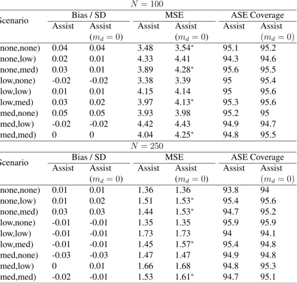
Simulation 1: Here we compare bias and MSE for three types of assisted estimators for difference in value. We use the assisted estimator, Vˆmˆd(d; ˆβ) with mˆd, an estimator of E[µ2(H2, d2(H2))|H1, A1], and Vˆ0(d; ˆβ), to estimate the contrast between embedded policies (1,1,1) and (0,0,0). We also consider Vˆmd(d; ˆβ) in which md is the unknown

(30)

prac-tice the optimalmdwill be unknown. The coverage of confidence intervals based on the

(31)

T able 2.1: Simulat ion 1: Statistical properties of the assisted estimators of the contrast between v alues of policies (1,1,1) and (0,0,0). Oracle = contrast estimator based on ˆVm d ( d ; ˆ_β) with the true optimal md . Assist = contrast estimator based on ˆVˆm d ( d ; ˆ_β) with a w orking estimate of the optimal md . Assist ( md = 0 ) = contrast estimator based on ˆV0 ( d ; ˆβ) . The displayed numbers for confidence interv al co v erage are the co v erage proportion × 100. An Asterisk indicates that the MSE of Oracle or Assist ( m d = 0 ) is significantly dif ferent from MSE of Assist (at 0 . 05 le v el). N = 100 Scenario T rue V alue Bias / SD MSE ASE Co v erage Oracle Assist Assist (m d = 0 ) Oracle Assist Assist (m d = 0 ) Assist Assist (m d = 0) (none,none) 0 0.04 0.04 0.04 3.51 ∗ 3.46 3.51 ∗ 95.7 95.4 (none,lo w) -2.4 0.01 0.01 0.01 4.26 4.26 4.31 95.1 95.6 (none,med) -5.2 0.03 0.03 0.01 3.94 3.93 4.3 ∗ 95.2 95.4 (lo w ,none) -1.4 -0.01 -0.01 -0.01 3.31 3.3 3.31 95.5 96.3 (lo w ,lo w) -3.8 0 0 0 4.08 4.14 4.12 95.5 95.9 (lo w ,med) -6.6 0.04 0.04 0.04 4.09 4.1 4.25 ∗ 95.6 96.3 (med,none) -3.6 0.03 0.03 0.03 3.96 3.93 3.96 95.9 95.4 (med,lo w) -6.0 -0.01 -0.01 -0.01 4.33 4.36 4.38 95.2 95.5 (med,med) -8.8 0.01 0.01 0 4.02 4.04 4.24 ∗ 95 95.7 N = 250 Scenario T rue V alue Bias / SD MSE ASE Co v erage Oracle Assist Assist (m d = 0 ) Oracle Assist Assist (m d = 0 ) Assist Assist (m d = 0) (none,none) 0 0 0 0 1.3 1.31 1.3 95 95 (none,lo w) -2.4 0.03 0.03 0.03 1.44 1.45 1.47 ∗ 95.1 95.1 (none,med) -5.2 0.03 0.02 0.02 1.4 1.4 1.48 ∗ 94.6 95.6 (lo w ,none) -1.4 -0.01 -0.01 -0.01 1.31 1.32 1.31 95.7 95.6 (lo w ,lo w) -3.8 -0.02 -0.02 -0.02 1.69 1.71 1.71 93.2 93.6 (lo w ,med) -6.6 0 -0.01 0 1.42 1.42 1.54 ∗ 95.3 95.2 (med,none) -3.6 -0.03 -0.03 -0.03 1.38 1.38 1.38 95.2 95.1 (med,lo w) -6.0 0 0 0.01 1.64 1.64 1.67 94.8 95 (med,med) -8.8 -0.02 -0.02 -0.01 1.55 1.55 1.63 ∗ 94.8 94.7

(32)

The simulation results with N = 100 and N = 250 are shown in Table 2.1. Based on the ratio of bias and standard deviation, we conclude that, as expected, the assisted estimators provide an unbiased estimate of the contrast between policies. The MSEs of all the three estimators are similar;Vˆmˆd(d; ˆβ)tends to be slightly more efficient thanVˆ0(d; ˆβ). The coverage of the confidence intervals based on the asymptotic standard errors is close to 95% in all cases.

In the appendix we provide additional simulations; these simulations illustrate that ˆ

Vmˆd(d; ˆβ)will provide a noticeable efficiency improvement overVˆ0(d; ˆβ)in some extreme settings. However, in most practical scenarios, a sophisticated chosenmddoes not

substan-tially improve the efficiency overmd ≡ 0; therefore for simplicity we recommend using

the assisted estimator withmd≡0.

Simulation 2: Here we assess the robustness via the bias, MSE and confidence inter-val coverage provided by the assisted estimators to misspecification of the SNMM. As a comparison we consider estimators from the marginal mean model [41] as these estimators do not require the SNMM. The marginal mean models are estimated via a non-parametric inverse-weighted estimator. Note that when the goal is to evaluate the difference between two policies, the estimators in [46] under particular choices of nuisance functions reduce to the marginal mean model estimators.

ˆ

Vmˆd(d; ˆβ) is estimated with two differently mis-specified SNMMs in addition to the correctly specified SNMM. The true SNMM is implied by the generative model in (2.5), i.e.,µ1(H1, A1) =A1(1, X1T)β1, µ2(H2, A2) =A2(1, X2T, A1, R, RX2T, RA2)β2. The first mis-specification of the SNMM excludes X11 from the model for µ1(H1, A1) and ex-cludesX21, RX21 from the model for µ2(H2, A2)(denoted as Assist2 in Table 2.2). The second mis-specification models µ1(H1, A1) as A1(1, X1∗T)β1 and models µ2(H2, A2) as

A2(1, X2∗T)β2, whereX1∗andX2∗are 3-dimensional and 7-dimensional covariates (denoted as Assist3 in Table 2.2). X₁∗ and X₂∗ generated independently of all the other covariates; the dimensions ofX₁∗andX₂∗are chosen so that the model complexity is the same as in the correctly specified SNMM.

We focus on the estimation of two contrasts: the first is the contrast between the policies (1,1,1) and (0,0,0), and the second is the contrast between a “tailored” treatment policy and the policy (0,0,0). This tailored treatment policy assigns a1 = 1 if X13 > 0; a2 = 1 to all early responders and a2 = 1 to early non-responders if X21 < 0. In each of the nine simulation scenarios we compare the marginal-mean-model-based estimator with the assisted estimators for three differently specified SNMMs.

(33)

T able 2.2: Simulation 2: Comparison between the mar ginal-mean-model-based estimators and the assiste d estimators , with respect to the performance in estimating the polic y contrasts, with N = 100 . MM = Mar ginal-mean-model-based estimator . Assist1 = Assisted estimator with correctly specified SNMM. Assist2 = Assisted estimator with mis-specified SNMM that excludes X11 ,X 21 ,R X21 . Assist3 = Assisted estimator with mis-specified SNMM that excludes all the co v ariates interacting with treatments. Bias significantly dif ferent from 0, and co v erage proportion significantly dif ferent from 95%, are mark ed with an asterisk. Relati v e MSE is calculated as the ratio of MSE with that of MM. N = 100 Estimation of the first contrast,(1, 1, 1) vs (0,0,0) Scenario Bias x 100 Co v erage of 95% CI x 100 Relati v e MSE MM Assist1 Assist2 Assist3 MM Assist1 Assist2 Assist3 Assist1 Assist2 Assist3 (none,none) 2.4 4.9 5.2 4.9 95.2 96.2 96 96.1 0.94 0.93 0.99 (none,lo w) 5.8 4.6 4.7 6 94.5 96 95.4 95.2 0.95 0.94 1.04 (none,med) 12 -6.8 -6.8 -2.6 93.6 ∗ 93.9 93.6 ∗ 94.6 0.95 0.95 1.01 (lo w ,none) -1.9 2.5 1.7 4.8 95.6 94.6 94 95 1.01 1.01 1.09 (lo w ,lo w) -12.5 -10.8 -11 -10.3 94.3 94.5 93.5 ∗ 94.6 0.92 0.92 0.97 (lo w ,med) 11 -9.9 -10.4 -5.8 93.9 94.8 94.7 95.5 0.84 0.84 0.93 (med,none) 8.9 4.2 5.4 3.4 95.5 95.9 95.3 96.2 0.89 0.87 0.89 (med,lo w) 9.7 -1.9 -2.7 -7.1 94.3 94.8 94.1 94.9 0.85 0.85 0.93 (med,med) 28.9 ∗ 4.2 5.4 4.7 93.7 94.9 95.2 94.9 0.8 0.79 0.85 Estimation of the second contrast, the tailored polic y vs (0,0,0) Scenario Bias x 100 Co v erage of 95% CI x 100 Relati v e MSE MM Assist1 Assist2 Assist3 MM Assist1 Assist2 Assist3 Assist1 Assist2 Assist3 (none,none) 6 1 2.4 2.3 96.2 97 ∗ 96.6 ∗ 96.1 0.78 0.76 0.57 (none,lo w) 6.4 4.8 -2.8 16.7 ∗ 95.6 96 95.7 94.7 0.79 0.77 0.59 (none,med) 11.5 -2.8 -22.1 ∗ -43.9 ∗ 94.9 95.8 95.1 94.4 0.78 0.77 0.67 (lo w ,none) 5.3 11.2 ∗ 9.7 42.9 ∗ 95.5 95.3 94.8 93.8 0.81 0.8 0.69 (lo w ,lo w) -7.3 -6.3 -15.1 ∗ 46.3 ∗ 93.9 95.3 93.9 95 0.77 0.74 0.59 (lo w ,med) 6.7 -1.8 -23.6 ∗ -2.8 94 96.3 94.9 95.7 0.7 0.69 0.5 (med,none) 9.3 8 9.1 50 ∗ 95.9 96.5 ∗ 95.8 95.4 0.76 0.74 0.57 (med,lo w) 13.7 ∗ 9.4 -0.3 53.3 ∗ 93.2 ∗ 95 95.2 94.1 0.7 0.67 0.57 (med,med) 24.7 ∗ 5.2 -15.1 ∗ 9.9 ∗ 93.1 ∗ 95.5 95.3 95.6 0.66 0.64 0.49

(34)

T able 2.3: Simulation 2: Comparison between the mar ginal-mean-model-based estimators and the assiste d estimators , with respect to the performance in estimating the polic y contrasts, with N = 250 . MM = Mar ginal-mean-model-based estimator . Assist1 = Assisted estimator with correctly specified SNMM. Assist2 = Assisted estimator with mis-specified SNMM that excludes X11 ,X 21 ,R X21 . Assist3 = Assisted estimator with mis-specified SNMM that excludes all the co v ariates interacting with treatments. Bias significantly dif ferent from 0, and co v erage proportion significantly dif ferent from 95%, are mark ed with an asterisk. Relati v e MSE is calculated as the ratio of MSE with that of MM. N = 250 Estimation of the first contrast,(1, 1, 1) vs (0,0,0) Scenario Bias x 100 Co v erage of 95% CI x 100 Relati v e MSE MM Assist1 Assist2 Assist3 MM Assist1 Assist2 Assist3 Assist1 Assist2 Assist3 (none,none) 2.6 4.7 4.4 4.8 93.5 ∗ 94.6 94.4 94.4 0.87 0.86 0.89 (none,lo w) 2 1.5 1.6 2.5 93.8 94.7 94.5 94.6 0.82 0.81 0.87 (none,med) 7.2 -1.2 -1.4 0.3 94.6 94.7 94.9 94.9 0.82 0.83 0.85 (lo w ,none) -4.6 -2.4 -3.3 -3.8 95.2 95.1 95 95.3 0.83 0.83 0.86 (lo w ,lo w) -5.1 -6 -5.8 -6.4 94.5 93.9 93.6 ∗ 93.8 0.87 0.87 0.89 (lo w ,med) 6 -0.3 -0.5 1.3 96 95.4 95.4 95.8 0.79 0.8 0.84 (med,none) -2.3 -1.3 -1.8 -1.1 94.5 94.3 94.3 95.9 0.75 0.76 0.78 (med,lo w) 9.3 ∗ 7.6 7.9 8.1 94.4 94.5 94.3 94.1 0.79 0.79 0.8 (med,med) 20.6 ∗ 11.2 ∗ 10.6 ∗ 14.3 ∗ 94.5 94.5 93.7 94.2 0.73 0.74 0.78 Estimation of the second contrast, the tailored polic y vs (0,0,0) Scenario Bias x 100 Co v erage of 95% CI x 100 Relati v e MSE MM Assist1 Assist2 Assist3 MM Assist1 Assist2 Assist3 Assist1 Assist2 Assist3 (none,none) -0.8 0.2 -0.2 2.3 95.1 93.6 ∗ 93.3 ∗ 95.4 0.69 0.67 0.48 (none,lo w) 0.2 0.5 -7.3 ∗ 13.2 ∗ 93.6 ∗ 94.7 94.3 94.9 0.65 0.64 0.46 (none,med) 6.7 0.9 -20 ∗ -39.5 ∗ 93.8 94.6 93.7 92.8 ∗ 0.69 0.71 0.58 (lo w ,none) -1.6 0.1 -1 38.5 ∗ 95.1 95.1 95.1 92.4 ∗ 0.67 0.66 0.6 (lo w ,lo w) -3.8 -1.5 -9.2 ∗ 49.1 ∗ 95.5 94.8 94.9 91.5 ∗ 0.68 0.68 0.62 (lo w ,med) 0.7 -0.5 -21.9 ∗ -0.7 95.1 95.2 94.7 96 0.68 0.7 0.45 (med,none) 2 3.6 2.4 46.9 ∗ 95.3 94.9 95.4 91.1 ∗ 0.6 0.59 0.55 (med,lo w) 10.4 ∗ 7.3 ∗ -0.5 63.7 ∗ 94.4 94.6 94.8 88.8 ∗ 0.62 0.6 0.65 (med,med) 8.7 ∗ 6.7 -15 ∗ 15.3 ∗ 94.7 95.4 94.9 94.1 0.64 0.62 0.46

(35)

The experiment results whenN = 100are shown in Table2.2; results forN = 250are shown in Table2.3. Instead of the MSE of the estimators, we present the relative MSE of the assisted estimators, with the MSE of the marginal-mean-model-based estimator (MM) as the reference. From the simulation results withN = 100, we found that, for the compar-ison between the two embedded policies, the assisted estimators with correctly specified SNMM outperform MM in terms of the MSE in most cases; mis-specifying the SNMM does not seem to introduce bias, but severe mis-specification (Assist3 in the Table) can lead to lower efficiency, and sometimes can even cause the assisted estimators to have a larger MSE than MM. For the comparison between the tailored policy and the reference policy, the assisted estimators with correctly specified SNMM outperform MM in terms of the MSE, and the advantage is greater than that of the first contrast. Mis-specifying the SNMM introduces bias; in particular, severe mis-specification (Assist3) leads to consid-erable bias. However, this bias does not seem to greatly impact the performance of the confidence interval. Interestingly, for the estimation of this contrast, mis-specifying the SNMM may even result in a smaller MSE despite of the bias, due to a smaller standard deviation in the estimate.

With a larger sample size (N = 250 as compared to N = 100), the advantage of the assisted estimators in terms of having a lower MSE than the marginal-mean-model-based estimators is more evident. Similar to the N = 100 experiments, mis-specifying the SNMM introduces bias in some scenarios, but even in those scenarios the performance of the assisted estimators in terms of the MSE does not worsen, because reduction in the variance dominates the bias-variance tradeoff. We notice that under the most severe mis-specification of SNMM (Assist3), the confidence interval of the contrast between the tai-lored policy and the policy (0,0,0)has noticeable under-coverage. However, we expect that in practice, such severe mis-specification, which fails to use any variable correlated with the variables in the true SNMM, might be unlikely to happen.

2.5 Illustration with the ExTENd Data

The ExTENd study (see Figure 2.1) includes 302 participants, with 49 participants drop-ping out prior to experiencing two heavy drinking days. These participants are removed from our analysis as they did not experience the first randomization and both they and the clinicians were blind to this randomization. Only three participants dropped out during the first treatment stage after experiencing two heavy drinking days. The data from these participants is also removed for simplicity. Thus the data we analyze has a sample size of 250.