by
Chua Lai Choon
A Dissertation Presented to the
DEPARTMENT OF STATISTICS AND APPLIED PROBABILITY NATIONAL UNIVERSITY OF SINGAPORE
In Partial Fulfillment of the Requirements for the Degree of
DOCTOR OF PHILOSOPHY
07 January 2012
Advisor
Professor Chen Zehua
National University of Singapore
To my wife, Bi and my daughters, Qing and Min.
I would like to take this opportunity to express my indebtedness and gratitude to all the people who have helped me made this thesis possible. I have benefited from their wisdom, generosity, patience and continuous support.
I am most grateful to Professor Chen Zehua, my supervisor and mentor, for his guid-ance and insightful sharing throughout this endeavour. Professor Chen first taught me Time Series in 2004 when I pursue my Master in Statistics and later in Survival Analysis in 2009 when I embark on this programme. I was not only impressed with Professor Chen’s encyclopedic erudition and versatility but was also in awe with his ability to de-liver complex concepts in simple terms. More importantly, Professor Chen ensures that his students received the concepts he delivered. I will always remember his simple but golden advice on getting to the “root” of a concept and how it can serve as a launching pad to more ideas. It was based on this that our thesis evolved. I am thankful that Professor Chen willingly took me under his wings and facilitated a learning experience that is filled with agonies and gratifications, as well as one that is enriching, endearing and fun. He had definitely rekindled the scholastic ability in me. Professor Chen has also been a great confidante and a pillar of strength. It really is an honour to be his student.
I am also very grateful to Professor Bai Zhidong, Professor Chan Hock Peng, Asso-ciate Professor Zhang Jin-Ting and Professor Howell Tong. I have benefited from their modules and their teaching have equipped and reinforced fundamental skills of statistics in me. The sharing of their experiences had impacted me positively and helped me set realistic expectations throughout this journey. Thanks also to all other faculty members and staffs of the Department of Statistics and Applied Probability for making this expe-rience an enriching one.
I would also like to thank my sponsor - The Ministry of Education - for this oppor-tunity to develop myself and to realize my potential. In particular, I would like to thank my superiors, Mr Tang Tuck Weng, Mr Chee Hong Tat, Mr Lau Peet Meng, Ms Lee Shiao Wei, Mr Chua Boon Wee for their strong recommendations and our peer leader, Dr Teh Laik Woon, for his useful advice and referral.
Last but not least, to my enlarged family, thank you for the patience and support.
I look forward to apply all the learning from this rigorous research and contribute positively to the work of the Ministry of Education - to enhance the quality of education in Singapore and to help our children realize their fullest potential.
This thesis focuses on one of the most important aspect of statistics - variable selection. The role of variable selection cannot be over emphasized with increasing number of pre-dictor variables being collected and analyzed. Parsimonious model is much sought after and numerous variable selection procedures have been developed to achieve this. The penalized regression is one such procedure and is made popular with the wide spectrum of penalty functions to meet different data structures and the availability of efficient computational algorithms.
In this thesis, we provide a penalty function called the Minimax Concave Bridge Penalty (MCBP) for the implementation of penalized regression that will produce vari-able selection with desired properties and addresses the issue of separation in logistic regression problems - when one or more of the covariates perfectly predict the response. It is known that separation of data often occurs in small data sets with multinomial dependent response and leads to infinite parameter estimates which are of little use in model building. In fact, the chance of separation increases with increasing number of covariates and thus is an issue of concern in this modern era of high dimensional data. Our penalty function addresses this issue.
The MCBP function that we developed is a product that draws strengths from ex-isting penalty functions and is flexibly adapted to achieve the characteristics required of penalty function to possess the different desired properties of variable selection. It rides on the merits of the Minimax Concave Penalty (MCP) as well as Smoothly Clipped Absolute Deviation (SCAD) functions in terms of its oracle property and the Bridge penalty function,Lq; q <1, in terms of its ability to estimate non-zero parameters
with-out asymptotic bias while shrinking the estimates of zero regression parameters to 0 with positive probability.
The MCBP function is inevitably nonconvex and this translates to a nonconvex ob-jective function in penalized regression with MCBP function. Nonconvex optimization is numerically challenging and often leads to unstable solutions. In this thesis, we also provide a matching computation algorithm that befits the theoretical attractiveness of the MCBP function and one which will facilitate the fitting of MCBP models. The com-putation algorithm uses the concave-convex procedure to overcome the nonconvexity of the objective function.
Dedication ii Acknowledgements iii Abstract v Contents vii List of Tables x List of Figures xi 1 Introduction 1
1.1 High dimensional data . . . 1
1.2 Model selection . . . 4
1.3 Logistic Model and Separation . . . 9
1.4 New Penalty Function . . . 11
1.5 Thesis Outline . . . 12
2 Penalty Functions 14 2.1 Penalized Least Square . . . 15
2.2 Penalized Likelihood . . . 16 vii
2.3 Desired Properties of Penalty Function . . . 17
2.3.1 Sparsity, Continuity and Unbiasedness . . . 17
2.4 Some Penalty Functions . . . 20
2.4.1 L0 and Hard Thresholding . . . 21
2.4.2 Ridge and Bridge . . . 21
2.4.3 Lasso . . . 23
2.4.4 SCAD and MCP . . . 25
3 Separation and Existing Techniques 28 3.1 Separation . . . 28
3.2 Overcoming separation . . . 31
4 Minimax Concave Bridge Penalty Function 34 4.1 Motivation . . . 34
4.2 Basic Idea . . . 35
4.3 Minimax Concave Bridge Penalty . . . 37
4.4 Properties and Justifications . . . 40
5 Computation 43 5.1 Some methods on non-convex optimization . . . 43
5.1.1 Local Quadratic Approximation . . . 44
5.1.2 Local Linear Approximation . . . 45
5.2 Methodology for the computation of MCBP solution path . . . 47
5.2.1 CCCP . . . 48
5.2.2 Predictor-corrector algorithm . . . 49
5.3 Computational Algorithm . . . 50
5.3.3 MCBP Penalized GLM model . . . 53 5.4 Package mcbppath . . . 62
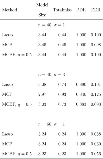
6 Numerical Study 68
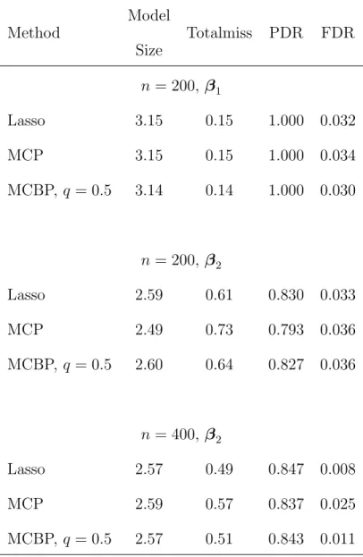
6.1 Case I, d < n . . . 69 6.2 Case II, d > n . . . 72 6.3 Analysis of CGEMS prostate cancer data . . . 76
7 Conclusion 85
7.1 Summary . . . 85 7.2 Future Work . . . 86
Bibliography 88
6.1 Output on Data Setting 1 (Linear regression) . . . 79
6.2 Output on Data Setting 2 (Logistic regression) . . . 80
6.3 Output on Data Setting 3 (Separation) . . . 81
6.4 Output on Data Setting 4 . . . 82
6.5 Output on Data Setting 5 . . . 83
6.6 Output on CGEMS data . . . 84
2.1 L0 and Hard, λ = 2, penalty functions (left panel) and PLS estimators
(right panel) . . . 22
2.2 Bridge, q = 0.5 and Ridge penalty functions (left panel) and PLS estima-tors (right panel) . . . 23
2.3 Lasso penalty functions (left panel) and PLS estimators (right panel) . . 24
2.4 SCAD, a= 3.7 and MCP, γ = 3.7 penalty functions (left panel) and PLS estimators (right panel) . . . 26
3.1 Configuration of data involving multinomial dependent response . . . 29
4.1 Minimax Concave Bridge Penalty function, γ = 3, r= 2/3 . . . 38
4.2 Plot of |β|+p0(|β|) . . . 40
4.3 PLS estimator or thresholding rule of MCBP function . . . 41
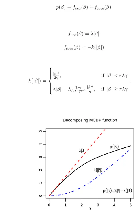
5.1 Decomposing MCBP into the sum of a concave and a convex function . . 52
Introduction
The advancement in technology and quantum leap in information management have led to the ubiquity of high dimensional data. A natural approach to the study of high di-mensional data is dimension reduction and the penalized approach has been proven to be a viable way. Separately, logistic regression is widely seen in statistics given the frequent encounter of binary or categorical responses. In fact, on many occasions, continuous responses are dichotomized and analyzed via logistic regression. Inherent in logistic re-gression, however, is the problem of separation which will result in indefinite parameter estimate. In the following, we give a brief introduction to the motivation behind our work and a sketch of our proposed method and the layout of the thesis.
1.1
High dimensional data
Prevalence of high dimensional data
Technological innovations and the development of biotechnology coupled with creative management of information have allowed massive complex data to be collected easily and
dimension, the number of covariates,p, is huge and is considerably larger than the num-ber of observations,n. Such data is also typically classified with the tag of smallnlargep.
High dimensional data is in abundance today. It can be found frequently in genomics such as gene expression and proteomics studies, biomedical imaging, signal processing, image analysis and finance, where the number of variables or parametersp can be much larger than sample size n [18]. For example, in genome-wide association study (GWAS) between phenotype such as body mass index and genotypes, a relatively small sample size is considered but hundreds of thousands of Single Nucleotide Polymorphism (SNPs) are typically investigated. Also, in disease classification using microarray gene expres-sion data, a small number of microarray chips each containing expresexpres-sion levels of tens of thousands of genes are usually involved [47] [21].
High dimensional data is also frequently encountered in health studies. For example, in a smoking cessation study, each of a few hundred participants is provided a hand-held computer, which is designed to randomly prompt the participants five to eight times per day over a period of about 50 days to provide 50 questions at each prompt to collect momentary assessment data. As such, the data consist of a few hundred of subjects and each of them may have more than ten thousand observed values [37]. Financial engineering and risk management data is likely small n large p. For example, the price of a stock depends not only on its past values, but also its bond and derivative prices. In addition, it depends on the prices of related companies and their derivatives, and on overall market conditions. Thus, the number of dimensions involved is huge.
Challenges of small
n
large
p
The characteristics of small n large p problem goes beyond the obvious - small sample size, n, and huge number of features, p. The dimensionality grows rapidly when in-teractions, which are necessary for many scientific endeavours, are considered. In high dimensional data, it is often believed that only a small fraction of the data is informative, which means that the number of causal or relevant features is only a few -sparsity. This is seen in genetic epidemiology study where the number of genes exhibiting a detectable association with a trait is extremely small. Indeed, for type I diabetes, only ten genes have exhibited a reproducible signal as illustrated by Wellcome Trust [50]. As such, studies on high dimensional data are like searching for a few needles hidden in a haystack -extracting a sparse number of features from the huge number of available features.
There are challenges of high dimensionality in feature selection. Firstly, the spurious correlation between a covariate and the response can be large because of the dimensional-ity even if all the features are stochastically independent. Secondly, in high dimensional feature space, important predictors can be highly correlated with some unimportant ones and this usually increases with dimensionality. This makes the partitioning of the impor-tant and the unimporimpor-tant predictors more difficult. Thirdly, the computation amount is prohibitive. The design matrix, X is rectangular with more columns than rows and the matrix XTX is huge and is singular. Fan and Lv provided comprehensive insights into the challenges of high dimensionality [19]. In addition, because p is larger than n, many off-shelf statistical methods are either inapplicable or inefficient. There is a need to overcome this curse of dimensionality as coined by Bellman [7].
1.2
Model selection
Goals of model selection
In general, there are two goals to model selection. They are
G1 To construct a good predictor. In this case, the interest is centered in the expected loss and the value of the coefficients is secondary.
G2 To give causal interpretations of the covariates on the response and to determine the relative importance of the covariates.
The former is the concept of persistency which was introduced by Greenshtein and Ritov [26] and the latter is the concept of consistency. G1 is generally the focus of machine learning problems such as tumor classifications based on microarray or asset allocations in finance, where the interests often center on the classification errors, or returns and risks of selected portfolios rather than the accuracy of estimated parameters. In studies when concise relationship among response and independent variables are required, G2 is the focus. Studies with such statistical endeavour generally involve health studies where one not only needs to identify risk factors but also to accurately assess their risk contributions. These are needed for prognosis and understanding the relative importance of risk factors. Approaches to model selection are dependent on the goal of the study.
Model Selection Approaches
Traditional model selection method such as stepwise procedure or best subset procedure is greedy and intensive in computation. They involve a combinatoric number of cases and is NP-hard. Though the criterion that is used in the selection of model with this method had been enhanced from AIC, BIC,Cp to EBIC which takes into consideration
high dimensionality, these methods remain infeasible for high dimensional data study. Furthermore, stepwise procedure does not guarantee that the exact model is among the model assessed. Such methods are more plausible for low dimensional data.
A model selection approach that has gained popularity and is viable for both low and high dimensional data is the penalized likelihood approach, or more generally, the penalized model selection. In such an approach, a penalty function with a tuning pa-rameter is added to the likelihood function to form the penalized likelihood. The tuning parameter, as the name suggests, is allowed to gradually decrease from a large value to a small value and this generates a sequence of nested models. With suitable penalty function, depending on data structure, the exact model is among the sequence of models and can be identified.
Penalty functions and computation
Different penalty functions were introduced to meet specific needs and challenges in penalized model selection. Briefly, the characteristics of the function will determine its performance in eliciting the model and its estimates as well as its ease of implementation. In the following, we will provide some common penalty functions and their properties.
Hoerl and Kennard [29], knowing that the best subset approach lacks stability [11], proposed the ridge regression (L2) to stabilize the estimates. Though computationally
friendly given its convexity, the ridge regression suffers from drawbacks of biasedness and does not have the function of variable selection. Frank and Friedman [24] intro-duced the bridge regression (Lq, 0 < q < 2) as a generalization of the ridge regression.
re-non-convex (q < 1) to convex (q ≥ 1) yields strikingly different competencies. Similar to ridge regression, bridge regression with q >1 does not shrink coefficients to zero and is not able to perform variable selection. For bridge regression with q < 1, the bridge estimator is able to distinguish between covariates whose coefficients are zeros and covari-ates whose coefficients are non-zero in situation when the number of covaricovari-ates is finite [34] as well as when the number of covariates increases to infinite with increasing sample size [30]. However, bridge regression remains unstable forq <1 and is biased whenq≥1.
Tibshirani [48] introduced the Least Absolute Shrinkage and Selection Operator, Lasso (L1) or equivalently Basis Pursuit [14] which does continuous shrinkage and
au-tomatic variable selection simultaneously. Lasso’s ability to shrink coefficient to zero is much welcomed in studies involving high dimension. As with most statistical methodolo-gies, a readily available efficient package is usually a catalyst to popular usage. Lasso is no otherwise. One of the main reason for Lasso’s popularity is the availability of efficient algorithms that traces its entire regularization path. Efron et. al. [16] and Osborne et. al. [42] showed that the solution path in the parameter space is piecewise linear. Efron et al. went further and used the idea of equiangular vector to develop the LARS algorithm to trace the entire path efficiently. Separately, Park and Hastie [43] use the predictor and corrector approach of convex optimization and intuitive choices of step length to generate the entire path with a much reduced number of iterations.
As mentioned earlier, Lasso’s ability to handle small n large p study and produce sparse models for easy interpretation are the main reasons for its continuous presence in statistical analysis especially in exploratory studies involving large number of covariates.
So important is Lasso that many studies were devoted to uncover the behaviour of Lasso estimate as the number of covariates grows. Zhao and Yu [57] as well as Zou [59] found that the sparsity pattern of the Lasso estimator can only be asymptotically identical to the true sparsity pattern if the design matrix satisfies the so called irrepresentable condition, a condition which can be easily violated in the presence of highly correlated variables. Meinshausen and Yu [39] further relaxed the irrepresentable condition and con-cluded that Lasso will select all important variables with high probability. Separately, Zou [59] and Wang et. al. [52] noted that if an adaptive amount of shrinkage is allowed for each regression coefficient according to its estimated relative importance, that is, not subjecting the same amount of shrinkage to each coefficient, then the resulting estimator can be as efficient as the oracle. All these findings endorse Lasso’s rigour in producing consistent selection and deeply entrenched its popularity with statisticians. Despite its popularity, Lasso’s inability to stay unbiased for large coefficient due to excessive penalty for large values of the coefficient remains a concern.
Fan and Li [17] proposed a unified approach via nonconcave penalized likelihood to simultaneously select and estimate the coefficients without the inherent shortcoming of bias in Lasso while still retaining the good features of the best subset selection and the ridge regression. They advocated that the penalized likelihood should also produce sparse solutions, ensure continuity of the selected models and have unbiased estimates for large coefficients - properties that have become synonymous with a good penalized variable selection procedure. Fan and Li further derived the conditions for such a penalty function to possess these properties and developed the Smoothly Clipped Absolute De-viation (SCAD) penalty function. For SCAD, it had been shown that its estimates have an oracle property in terms of selecting the correct subset model and estimating the true
The nonconcave penalty functions that satisfy the conditions spelt out by Fan and Li will necessarily have to be singular and nonconvex. This implies that conventional convex optimization algorithms are not applicable. Fan and Li suggested using the lo-cal quadratic approximation (LQA) to lolo-cally approximate the penalty function by a quadratic function iteratively. With the aid of the LQA, the optimization of penalized likelihood function can be carried out using a modified Newton Raphson algorithm. How-ever, as pointed out by Fan and Li, the LQA algorithm shares a drawback of backward stepwise variable selection, that is, a covariate that is being removed in any step in the LQA algorithm will not be included in the final selected model. Though Hunter and Li [31] attempted to address this issue by optimizing a slightly perturbed version of LQA, the choice of the size of pertubation remains unanswered. Subsequently, Zou and Li [61] proposed a unified algorithm to solve nonconcave penalized likelihood based on Lo-cal Linear Approximation (LLA). Similar to the LQA algorithm, the maximization of the penalized likelihood can be solved iteratively till it converges using the unpenalized maximum likelihood estimate as the initial value. The LLA algorithm inherits the good features of Lasso in terms of computational efficiency and therefore efficient algorithm such as LARS can be used. With computational algorithms developed for its use, SCAD, with its impeccable statistical properties also enjoy wide popularity especially in situa-tion where more refined selecsitua-tion is required.
Zhang [55] developed the MC+ method which shed deep and new insights into non-concave penalized models. The penalty function in Zhang’s method is known as the minimax concave penalty (MCP) function which mirrors the properties of the SCAD
penalty. MCP provides sparse convexity to the broadest extent by minimizing the max-imum concavity. It has a single knot compared to the double knot in SCAD and this gives it the versatility and simplicity over SCAD. In addition, Zhang proposes the pe-nalized linear unbiased selection (PLUS) algorithm to efficiently compute the estimate of the coefficients. The PLUS algorithm differs from most existing nonconvex optimiza-tion algorithms in its approach, computing exact local optimizers instead of iteratively approximating them. It has been shown that PLUS has the same efficiency as LARS.
Many penalty functions were developed using a combination of basic penalty functions such as those listed above. Such penalty functions make good use of the characteristics of each of the basic penalty function to achieve specific purposes. For example, the Elastic Net [60], which is a combination of Lasso and Ridge penalty, can be perceived as a two stage procedure which facilitates the selection of highly correlated predictors as a group -either all in together or all out together. Similarly, the two stage procedure proposed by Zhao and Chen [56] make use of Lasso’s efficiency in achieving sparsity to perform initial screening and utilizes SCAD to perform finer selection. Other penalty functions are a convolution of others. Particularly, SCAD has a Lasso for small parameter to achieve sparsity and a constant penalty for large parameter to achieve unbiasedness.
1.3
Logistic Model and Separation
Logistic regression is probably the most common statistical analysis after linear regres-sion. Its widespread use can be attributed to the high occurrences of binary or categorical responses. Common examples that require the use of logistic regression include the anal-ysis of the presence of disease (binary) in biomedical research as well as the analanal-ysis
continuous responses are dichotomized and analyzed via logistic regression.
With its prevalent use, it is important for one to be aware of the common pitfalls in logistic regression analysis. One of the potential problems when running a logistic regression is separation. It is an issue that commonly occurs in small or sparse datasets with highly predictive covariates as well as in data which possesses ceiling or floor ef-fect. Separation, using traditional likelihood approach, results in indefinite parameter estimate and is a challenge to many researchers. In some cases, researchers are forced to choose between omitting clearly important covariates and undertaking posthoc data or estimation corrections leading to non-optimal analysis. In extreme scenarios, separation may lead to the discontinuation of a study.
In terms of penalized model selection that addresses separation, the most popular one is Firth’s [22] penalized maximum likelihood estimator which reduces the bias of maximum likelihood estimates and ensures the existence of estimates by removing the first-order bias at each iteration step. Firth’s approach, in exponential families with canonical parameterization, is equivalent to penalizing the likelihood with the Jeffreys invariant prior, 12log|I(θ)|, where θ is the parameter vector and I(θ) is the Fisher in-formation matrix [33]. Although Firth’s approach has been shown empirically, by Bull et. al. [12] and Heinze and Schemper [27], to be superior to other methods which over-come separation in small samples and Firth’s estimator was equivalent to the maximum likelihood estimator as sample size increases, the asymptotic properties of its penalized likelihood estimator have not been examined. Riding on Firth’s approach, Gao and Shen [25] propose a double penalty by introducing a second penalty term to Firth’s penalty.
They added a ridge penalty which forces the parameters to spherical restriction and thereby achieving asymptotic consistency under mild regularity conditions.
1.4
New Penalty Function
We develop a penalty function that possesses desired properties in variable selection such as sparsity, continuity and unbiasedness; able to automatically select and estimate coef-ficients and is capable of handling separation in data. A synthesis of the characteristic of each of the different penalty functions and an in-depth understanding of the issue of separation in data provided us with the fundamentals to construct our penalty function. The basic idea requires covariates that lead to separation to be sufficiently penalized and yet not too much to maintain unbiasedness. The ability of bridge regression (q < 1) to estimate non-zero regression parameters at the usual rate without asymptotic bias while shrinking the estimates of zero regression parameters to 0 with positive probability [34] [30] provided us with a viable way to achieve the balance we are seeking.
Briefly, our proposed penalty function - Minimax Concave Bridge Penalty (MCBP) function, has a Lq, q <1 penalty instead of a constant penalty function in MCP for large
parameter. It is envisaged that MCBP function will yield estimators that have the oracle property and is able to address the issue of data with separation at the same time. MCBP function will necessarily need to be non-convex. Non-convex optimization has always been a challenge and this practical issue has, at times, lead to a compromise in the pursuit of sound rigorous statistical methodologies. In this thesis, we also propose an algorithm to overcome this computational challenge via the ideas of predictor and corrector approach [43] and the concave and convex procedure [54]. Last but not least, as a by-product,
selection and this facilitates understanding of their theoretical properties and increases confidence of its usage. The simultaneous selection and estimation of the coefficients allows the distribution of the estimates to be determined and this enables the asymptotic behaviour of the estimates to be established.
1.5
Thesis Outline
In Chapter 2, we provide an overview of the evolution of the penalized selection proce-dure. We see how penalty function is applied in least square selection procedure followed by its natural extension to the penalized likelihood selection procedure. We will also deliberate on the desired properties of penalty functions and how some of the common penalty functions - both convex and non-convex measure up in these desired properties. In Chapter 3, we discuss separation in data. Particularly, we share how separation arises and the consequences of it. We will share some existing methods of handling separation in data and highlight the importance of resolving it.
In Chapter 4, we propose our penalty function. We will provide insights into the development of the proposed penalty function and justify its strengths and properties. In Chapter 5, we lay down the details of the algorithm for the computation. We perceive the non-convex penalized likelihood as a sum of concave and convex functions and apply the Concave and Convex Procedure with suitable transformations to transform it into an adaptive Lasso and use the predictor and corrector approach to facilitate the optimiza-tion of our penalized likelihood.
In Chapter 6, we subject our penalty function to test with both simulated and real data. We make comparison of the performance of our proposed penalty function with other penalty functions in terms of selection consistency. Finally, summary of the main points of the thesis and future directions are shared in Chapter 7.
Penalty Functions
Parsimonious models are desirable [49] [8]. They are simpler and easier to interpret. The availability of massive data has heightened interest in the development of methodologies in dimension reduction. Penalized model selection, a viable approach to handling large number of covariates, also grow in tandem and different penalty functions have been introduced to elicit the true model for different constructs of data sets.
In this chapter, we will provide an overview of the evolution of the penalized model selection. We will see how the penalty function is applied in least square selection pro-cedure followed by its natural extension to the penalized likelihood selection propro-cedure. We will also deliberate on the desired properties of penalty functions and how some of the common penalty functions, both convex and non-convex, measure up in these desired properties.
2.1
Penalized Least Square
The Ordinary Least Square (OLS) regression is unequivocally the first introduction to statistical modelling for most people. Consider the linear regression model
yi =xTi β+i, i= 1,2, . . . , n
whereyi is the response variable,xi is a d-dimensional vector of fixed independent
vari-ables, β = (β1, . . . , βd)T is an unknown d-dimensional vector of regression coefficients
and i’s are i.i.d random noises with mean zero and variance σ2. The OLS estimate is
obtained by minimizing the residual square error:
min β n X i=1 (yi−xTi β) 2
Despite its shortcomings in prediction accuracy and parsimony [48], OLS is still much alive for its simplicity and easiness in comprehension. However, the ubiquity of high di-mensional data with smallnlargeplimited the application of OLS for the obvious reason of having too many parameters to estimate with few observations. Furthermore, multi-collinearity, a frequently occurring phenomena especially in high dimensional data will render the matrix XTX to be singular which in turn makes the inverting of the matrix impossible. A possible remedy to this is to use ridge regression [29] where a constantλ is added to the diagonal elements ofXTX to make the matrix non-singular. This is equiv-alent to adding a penalty to the model. Hence, taking a leaf from optimization problem with constraints, a penalized least square regression - an OLS with additional constraints can be a viable approach to restrict parameter estimates and achieve model selection. Thus, a penalized least square estimate is the solution to the following optimization problem:
min β n X i=1 (yi−xTi β) 2 subject to d X j=1 pλj(|βj|)≤t
wherepλj(.) is a penalty function.
An alternate form of penalized least square regression could be the following:
min β 1 n n X i=1 (yi−xTi β) 2 + d X j=1 pλj(|βj|) (2.1)
The introduction of the additional constraint, called the penalty function, inevitably restrict the possibilities of the estimate. The dependency of the penalty function on j allows for the manipulation of model complexity. In particular, with careful selection of penalty function, the penalized least square regression is able to shrink coefficient to zero value and thus achieving model selection.
2.2
Penalized Likelihood
For generalized linear models, statistical inferences are based on underlying likelihood functions. Suppose that the data (xi, Yi) are collected independently. Conditioning on
xi, Yi has a density fi(g(xTβ),yi), where g is a known link function. The maximum
likelihood estimate is the solution to
max β 1 n n X i=1 logfi(g(xTiβ), yi).
Thus, similar to penalized least square, a natural extension into likelihood-based generalized linear model produces the penalized (maximum) likelihood estimate which is the solution to
max β 1 n n X i=1 logfi(g(xTi β),yi)− d X j=1 pλj(|βj|) which is equivalent to min β − 1 n n X i=1 logfi(g(xTi β),yi) + d X j=1 pλj(|βj|)
In particular, for logistic regression, the penalized likelihood is
min β − 1 n n X i=1 [yi(xTi β)−log[1 + exp(x T i β)]] + d X j=1 pλj(|βj|)
With suitable penalty function, the penalized likelihood can be used to perform model selection. It can simultaneously perfom variable selection and parameter estimation and these facilitate the establishment of the distribution of the resulting estimators and the study of their asymptotic properties.
2.3
Desired Properties of Penalty Function
Penalized model selection is indeed an extension of OLS and maximum likelihood. It has an additional constraint, a penalty function, to adhere to. What characteristics should penalty functions possess to enable them to perform selection and estimation - a highly valued competency in model selection? In the following, we list a few logical and desired outcomes in model selection as well as the conditions that penalty functions need to have to achieve these desired outcomes in model selection.
2.3.1
Sparsity, Continuity and Unbiasedness
Fan and Li [17], in their introduction of the SCAD penalty function to overcome draw-backs of existing penalty functions, listed three main properties that estimators from a
(P1) Sparsity: The resulting estimator should automatically set small estimated coeffi-cients to zero to achieve model selection.
(P2) Continuity: The resulting model should be continuous from model to model to reduce instability in model prediction.
(P3) Unbiasedness: The resulting estimator is asymptotically unbiased.
Such properties will enable the attainment of the desired outcomes of model selec-tion. In sparsity, one is able to shrink coefficients to zero and achieve parsimony and this facilitates knowledge discovery from massive data. The unbiasedness property will improve accuracy and the continuity will ensure stability, providing continuous solution and avoid discrete jump that will lead to model variation.
The conditions for a penalty function to produce penalized estimator that have the properties of sparsity, continuity and unbiasedness are derived by Antoniadis [6] and Fan and Li [17]. The conditions involve the derivative ofpλ(.) and are namely
(C1) Sparsity: if minβ [|β|+p0λ(|β|)]>0.
(C2) Continuity: iff arg minβ [|β|+p0λ(|β|)] = 0.
(C3) Unbiasedness: if p0λ(|β|)→0 as |β| → ∞ .
Oracle Property
Apart from the sparsity, continuity and unbiased properties, Fan and Li also introduced the concept of oracle property in variable selection. It is observed that under certain regularity conditions, the rate of convergence for the penalized likelihood estimator is
dependent on the tuning parameter (λ) and with proper choice of the tuning parameter, the penalized likelihood estimator can be made to possess the oracle property - a desired property that implies that it will
(O1) estimate true parameters with zero value as zero with probability tending to 1 as n → ∞ (Sparsity );
(O2) estimate true parameters that are non-zero as well as when the correct submodel is known (Asymptotic normality ).
Formally, Fan and Li [18] expressed the oracle property in the following manner: Denote β0 to be the true value ofβ. Without loss of generality, assume that the first s components of β0, denoted by β01, are non-zero and do not vanish and the remaining d−s coefficients, denoted byβ02, are 0. Denote by
Σ = diag{p00λ 1(|β01|), . . . , p 00 λs(|β0s|)} and b= (p0λ 1(|β01|)sgn(β01), . . . , p 0 λs(|β0s|)sgn(β0s)) T Theorem 1
Assume that as n → ∞, min1≤j≤s|β0j|/λj → ∞ and the penalty function pλj(|βj|)
satisfies lim inf n→∞ lim infβj→0+ p0λ j(βj)/λj >0 Ifλj →0, p
n/dλj → ∞ and d5/n → 0 as n → ∞, then with probability tending to 1,
the rootn/d consistent local maximizers ˆβ= ( ˆβT1,βˆT2)T must satisfy:
positive definite symmetric matrix,
√
nAI−11/2{I1+ Σ}{βˆ1−β01+ (I1+ Σ)−1b}
D
→N(0,G)
whereI1 =I1(β01,0), the Fisher information knowing β02= 0
That is, a penalized likelihood estimator with oracle property will perform as well as the maximum likelihood estimates for estimating β1 knowing β2 = 0. It asymptotically correctly identifies the non-zero parameter and points to the true underlying model as well as attains an information bound mimicking that of an oracle estimator.
2.4
Some Penalty Functions
As the form of the penalty function determines the behaviour of the estimator, different penalty functions, each with its own characteristics, are introduced to meet different purposes and situations. Some penalty functions are a convolution of other penalty functions or a combination of a sequence of one penalty function followed by another. Such penalty functions exploit the characteristics of the basis penalty functions with the aim to achieve specific outcomes or to overcome unique underlying data structure. In the following, we list some penalty functions that usually form the basis for other penalty functions. We will only highlight the characteristics of each of the penalty functions and leave the discussion of the computation issue to Chapter 5.
2.4.1
L
0and Hard Thresholding
The entropy or theL0 penalty
pλ(|β|) =
1 2λ
2I{|β| 6= 0}
where I is the indicator function, makes the penalized least square (2.1) dependent on the size of the candidate model, m=Pd
j=1I{|βj| 6= 0}. For each m, the selected model
is the one with the minimum residual sum of squares. The selection of which m is then done through some criteria such as adjusted R2 or generalized cross-validation (GCV).
It has been shown that many of the popular variable selection criteria such as adjusted R2, GCV, RIC are asymptotically equivalent to (2.1) with the entropy penalty function
and with different λ [18] [23] [40]. Thus, the selection of variables via best subset can be done through the entropy or L0 penalty.
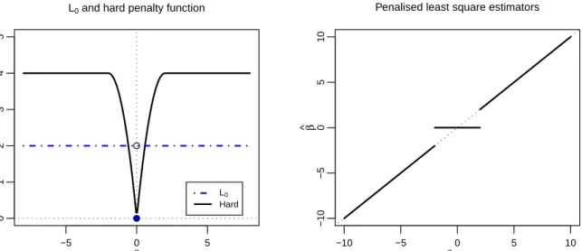
The hard thresholding penalty [5],
pλ(|β|) =λ2−(|β| −λ)2I{|β|< λ},
is smoother than theL0 penalty and will yield the same hard thresholding rule as theL0
penalty in (2.1) (See Figure 2.1).
These penalty functions, besides not being computationally tractable when the num-ber of covariates is large, will also not produce models that are continuous, leading to instability in model.
2.4.2
Ridge and Bridge
Ridge penalty was introduced by Hoerl and Kennard [29] to overcome the instability of estimates from best subset approach. Its penalty function is as follows:
−5 0 5 0 1 2 3 4 5 β p ( β )
L0 and hard penalty function
L0 Hard ● ● −10 −5 0 5 10 −10 −5 0 5 10 β ^ βOLS
Penalised least square estimators
Figure 2.1: L0 and Hard, λ= 2 penalty functions (left panel) and PLS estimators (right
panel)
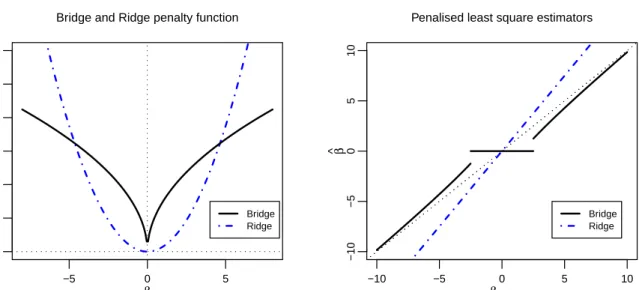
and is a special case of the more generic Bridge penalty function
pλ(|β|) =λ|β|q, q >0
introduced by Frank and Friedman [24] (See Figure 2.2).
The ridge penalty, though computationally friendly, suffers from drawbacks of being biased and does not perform model selection as it does not shrink coefficients to zero - an indispensable capability in dealing with high dimensional data. Similar to ridge regression, bridge regression with q > 1 does not perform variable selection. For bridge regression withq <1, the bridge estimator is able to distinguish between covariates whose coefficients are zeros and covariates whose coefficients are non-zero in situation when the number of covariates is finite [34] as well as when the number of covariates increases to infinite with increasing sample size [30]. In addition, Bridge regression remains not stable forq <1 and is biased when q ≥1.
−5 0 5 0 1 2 3 4 5 6 β p ( β )
Bridge and Ridge penalty function
Bridge Ridge −10 −5 0 5 10 −10 −5 0 5 10 β ^ βOLS
Penalised least square estimators
Bridge Ridge
Figure 2.2: Bridge, q= 0.5 and Ridge penalty functions (left panel) and PLS estimators (right panel)
2.4.3
Lasso
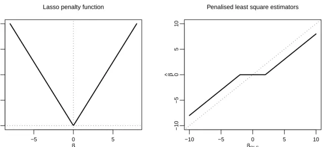
Lasso (Least Absolute Shrinkage Selection Operator), a special case of bridge penalty, was first introduced by Tibshirani [48] and has a L1 penalty
pλ(|β|) = λ d X
j=1
|βj|.
The resulting estimator from the Lasso penalty has both the sparsity and continuity properties but not the unbiasedness property. It is worth pointing out that Lasso could also be limited in the following situations as pointed out by Zou and Hastie [60]:
(a) In situations where d > n, Lasso selects at most n variables given the nature of the convex optimization problem and this is a limiting feature for variable selection procedure.
(b) When a group of variables are highly pairwise correlated, Lasso select only one variable from the group.
−5 0 5 0 2 4 6 8 β p ( β )
Lasso penalty function
−10 −5 0 5 10 −10 −5 0 5 10 β ^ βOLS
Penalised least square estimators
Figure 2.3: Lasso penalty functions (left panel) and PLS estimators (right panel)
(c) The prediction prowess of Lasso is overshadowed by ridge regression in situations where n > d.
Despite this, Lasso enjoys wide popularity because of its ability to select variables and its ease in implementation given its convexity. Lasso’s prevalence leads to many studies to uncover the behaviour of its estimates as the number of covariates grow. Zhao and Yu [57] and Zou [59] found that the sparsity pattern of the Lasso estimator can only be asymptotically identical to the true sparsity pattern if the design matrix satisfies the so called irrepresentable condition1, a condition which can easily be violated in the
presence of highly correlated variables. Meinshausen and Yu [39] further relaxed the irrepresentable condition and concluded that Lasso will select all important variables with high probability. Separately, Zou [59] and Wang et al. [52] noted that if an adaptive amount of shrinkage is allowed for each regression coefficient according to its estimated
1The irrepresentable condition is dependent on the covariance of the predictor variables and the
condition will hold if the total amount of an irrelevant covariate represented by the covariates in the true model did not reach 1. See [57] for formal representation of the irrepresentable condition.
relative importance, the resulting estimator can be as efficient as the oracle. All these findings endorse Lasso’s rigour to produce consistent selection secured its position as one of the most commonly used penalty function. However, Lasso’s inability to have unbiased estimators remains a concern.
2.4.4
SCAD and MCP
Fan and Li [17] proposed a unified approach via nonconcave penalized likelihood to simultaneously select and estimate the coefficients without the inherent shortcoming of biasedness in Lasso while still retaining the good features in Lasso. They introduced the Smoothly Clipped Absolute Deviation (SCAD) penalty function.
pλ(|β|) = λ|β|, if 0≤ |β|< λ
−|β|2−2(2a−aλ|β|1)+λ2, if λ≤ |β|< aλ
(a+1)λ2
2 , if |β| ≥aλ
This penalty function is constructed in such a way that it retains the good property of Lasso in sparsity with aL1 penalty for small parameter, a constant penalty for large
parameter to overcome the issue of bias and uses a quadratic spline at two knots λ and aλ, wherea >2, to generate a continuous differentiable penalty function.
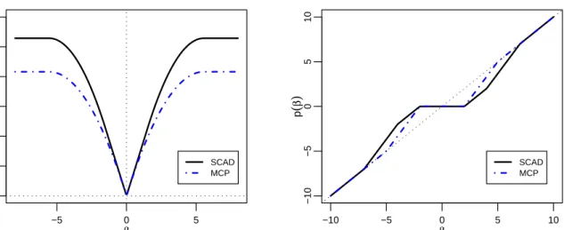
Although SCAD penalty function produces estimator that has all 3 properties, it is nonconvex. It is therefore more difficult than Lasso in terms of computation. Nonethe-less, the good statistical properties of SCAD motivated many algorithms to be developed and thus SCAD is also commonly used in model selection.
unbi-−5 0 5 0 1 2 3 4 5 6 β p ( β )
SCAD and MCP penalty function
SCAD MCP −10 −5 0 5 10 −10 −5 0 5 10 β p ( β )
Penalised least square estimators
SCAD MCP
Figure 2.4: SCAD, a = 3.7 and MCP, γ = 3.7 penalty functions (left panel) and PLS estimators (right panel)
asedness. It provides sparse convexity to the broadest extent by minimizing the maximum concavity. Following the conditions it needs to possess such properties, its penalty func-tion can be expressed asλR|β|
0 (1−
x
γλ)+dx which can be expressed as
pλ(|β|) = λ(|β| − |β|2λγ2), |β|< λγ λ2γ 2 , |β| ≥λγ
Visually, MCP is a refinement of SCAD where it uses a single knot rather than two to achieve the desired properties. A larger value of the tuning parameter γ affords less unbiasedness and more concavity. As such, MCP is “simpler” than SCAD in a way and in fact any similar penalty function within the region between the MCP and the SCAD, as shown in Figure 2.4, will have the desired properties. Nevertheless, the computation and analytical difficulties of such nonconvex minimization remain a concern.
There are penalty functions that are Lasso-like which make use of combinations of Lasso-type of penalty functions to address specific issues. An example is the Elastic Net proposed by Zou and Hasite [60], which is a combination of Lasso and Ridge penalty to address the issue of grouping of variables. It can be perceived as a two stage procedure which facilitate the selection of highly correlated predictors as a group - either all in together or all out together. There are also multiple-stage methods which make good use of each of the characteristics of the different Lasso-type of penalty functions to perform initial screening and final selection. One example is the two stage procedure proposed by Zhao and Chen [56] which makes use of Lasso’s efficiency in achieving sparsity to perform initial screening and utilizes the SCAD to perform finer selection. Other penalty func-tions are a convolution of others. Particularly, SCAD has a lasso for small parameters to achieve sparsity and a constant penalty for large parameter to maintain unbiasedness.
In summary, penalty function determines the behaviour of the estimator. With good understanding of the characteristics and properties of a basis of penalty functions, one can generate a wide spectrum of different penalty functions via composition or convolutions to meet different needs. It is with this understanding that we formulate our penalty function to overcome the prevalent problem of separation in logistic regression.
Separation and Existing Techniques
Logistic regression is probably the most common statistical analysis after linear regres-sion. Its widespread use could be attributed to the high occurrences of binary or cat-egorical responses. In fact, on many occasions, continuous responses are dichotomized and analyzed via logistic regression, making it pervasive in statistical analysis.
In this chapter, we will discuss separation, a common pitfall in logistic regression analysis. Particularly, we will highlight how separation arises and the consequences of it. We will also list some existing methods that help to ameliorate the issue of separation in data and emphasize the importance of resolving it.
3.1
Separation
According to Albert and Anderson [3], the configuration of data involving categorical response variable can be categorized into 3 mutually exclusive categories:
(a) Separation,
(b) Quasi-separation and
(c) Overlap
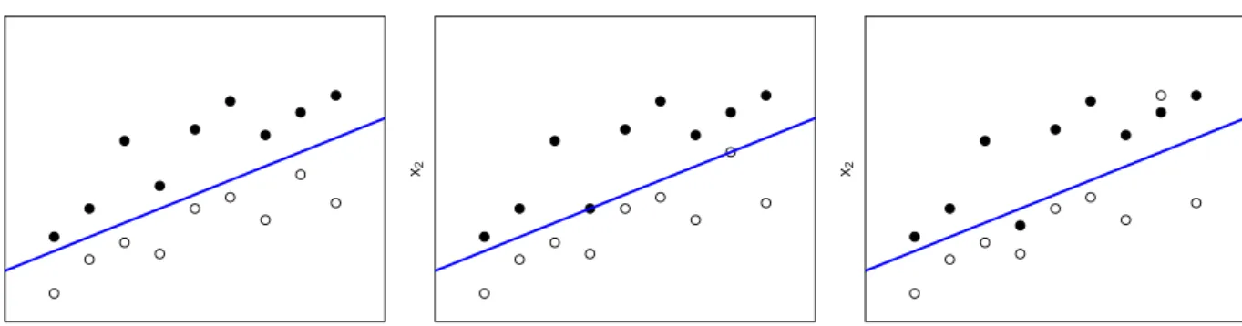
In particular, for the archetypical logistic regression model for a binary dependent variable, separation occurs when there exists a subvector of the covariates by which all subjects can be correctly classified in terms of their responses of either 0 or 1. This is equivalent to the existence of a hyperplane passing through the space of the covariates such that on one side of the hyperplane are observations with 0s’ while on the other side are observations with 1s’ as interpreted by Agresti [1]. Pictorially, it can be illustrated [46] as follows: ● ● ● ● ● ● ● ● ● ● ● ● ● ● ● ● ● ● x1 x2 Separation ● ● ● ● ● ● ● ● ● ● ● ● ● ● ● ● ● ● x1 x2 Quasi−separation ● ● ● ● ● ● ● ● ● ● ● ● ● ● ● ● ● ● x1 x2 Overlap
Figure 3.1: Configuration of data involving multinomial dependent response
That is, separation occurs when the categorical response can be perfectly separated by a single variable or a non-trivial linear combination of the variables (separating vari-ables) [36]. Quasi-separation occurs when the response variable are “almost” perfectly separated, with some responses lying on the line of separation generated from the sepa-rating variables.
In both separation and quasi-separation, the maximum likelihood estimates of the parameters associated with the separating variables are infinite. This is the main issue
population are finite [27]. This thorny problem, on many occasions, has often forced researchers to embark on difficult and consequential decisions due to ignorance or lack of skills to tackle it. In addition, it is worth pointing out that the actual estimates of parameter of the separating variables in most standard statistical software packages are dependent on the arbitrary choice of the convergence criteria for the estimation routine in the algorithm of the package. This, in the hand of unsuspecting researchers, can be pernicious and is undesirable.
Besides being pervasive in situations where data is sparse and strong relationships are present, separation can also be found in inconspicuous situations. In fact, Heinze and Schemper [27] showed that separation can actually be quite prevalent under a host of other conditions. In particular, they showed that separation can occur even when the underlying model parameters are low in absolute value. They also showed that the probability of separation is dependent on the number of dichotomous covariates, the magnitude of the odds ratios and the degree of balance in their distribution.
Furthermore, addressing the issue of separation in data is implicitly variable selec-tion. The importance of variable selection, especially in high-dimensional data space, cannot be overly emphasized. Hence, it is important that one is equipped with ways to overcome separation and best if one can have a method that not merely address the issue of separation but also possess the desired properties of variable selection.
3.2
Overcoming separation
Numerous approaches have been introduced and employed to handle data with sepa-ration. At the upstream is simple “solution” that includes increasing sample size or removing the separating variables that cause the problem or combining variables. There are also methodologies and approaches that are capable of overcoming separation and these include exact logistic regression, Jeffreys invariant prior and Firth’s method.
Upstream approaches are simple but are generally contentious and not preferred by many researchers. Increasing sample size, for example, is not always feasible particularly in observational or other non-experimental contexts and is likely to be subjected to query. On the other hand, omitting the separating variable that causes the problem but bearing a strong relationship to the response not only provide no information about the effect of this highly predictive variable but also does not allow the adjustment of the effects of other variables with respect to this separating variable. It is in fact a deliberate spec-ification bias. Another upstream approach, data manipulation, also has its drawbacks. Agresti and Yang [2] showed that simply adding a constant to ensure existence of esti-mates can have undesirable properties. Clogg et. al.’s [15] approach of adding artificial responses and non-responses and then analyzing the augmented data has been proven to be inferior [27].
Beyond upstream approaches, exact logistic regression was specifically developed to overcome separation. Briefly, exact logistic regression replaces the unsuitable maximum likelihood estimate with a median unbiased estimate. This, however, is computationally intensive and will fail when there are variables that lead to degenerate distributions of all sufficient statistics as illustrated by Heinze and Schemper [27].
Separately, Firth’s approach to reduce bias in maximum likelihood estimators is found to be particularly useful in addressing separation. Firth, unlike others preceding him, took a preventive approach instead of a corrective one by introducing a bias into the score function to reduce bias in maximum likelihood estimators. This approach removes the leading term in the asymptotic bias of the maximum likelihood estimator and thereby achieving bias reduction. Unlike corrective approaches, the preventive approach by Firth allows it to nip the problem at its bud and is useful in addressing separation where the parameter estimates are infinite.
Firth’s method of bias reduction, also known to be equivalent to Jeffreys invariant prior, has been comprehensively studied. Heinze and Schemper [27], with simulation, applied Firth’s method to logistic regression with separation in data and showed it to be better than other methods. Separately, Bull et. al. [12] extended Firth’s method in multinomial logistic regression and also proved it to be superior over other methods in small samples and Firth’s estimator was equivalent to the maximum likelihood estima-tor as sample size increases. Gao and Shen [25], through adaptation of Firth’s method, further showed that Firth’s method was asymptotically consistent.
There are other viable methods, often as a by product, that can overcome separation. Particularly, in glmpath algorithm, a ridge penalty with a finite small positive factor is added to L1 penalty to facilitate smooth computation and to avoid non-convergence.
The introduction of this ridge penalty with a small fixed tuning parameter prevents the parameter estimates from escalating to infinity and indirectly overcome separation, if any.
Addressing the issue of separation is not merely about producing finite parameter estimates for interpretation. It has far reaching ramifications if not adequately resolved. Overcoming separation also solve some common issues faced in statistical analysis. In particular, it permits Monte Carlo studies of small sample settings which generally results in frequent cases of separation to be performed. Studies involving bootstrapping which results in separation among resample even though there is no separation in the original sample will no more be a problem.
With this background, we aim to provide an alternate and competent penalty func-tion that will go beyond the addressing of separafunc-tion in data to one possessing desired properties in model selection and is computationally efficient in selecting variables in high dimensional feature space.
Minimax Concave Bridge Penalty
Function
Having reviewed the penalized approach to model selection and the issue with separation in logistic regression, we will lay out our proposed penalty function in this chapter. We will sketch the development of our proposed penalty function and discuss its associated desired properties in model selection with high-dimensional feature space which makes it superior over existing methods.
4.1
Motivation
The idea of this proposed penalty function stems from the work of Zhao and Chen [56] where they developed a two-stage penalized logistic regression approach to case-control genome-wide association study (GWAS). In their approach, Zhao and Chen first use the Lasso penalty to screen out apparently unrelated variables and reduce the number of variables to a tractable level. They subsequently apply the SCAD penalty to rank the variables which survive the initial screening to facilitate the final model selection. A
Jeffreys invariant prior penalty was added to the SCAD penalty to manage the issue of separation or quasi-separation which is prevalent in logistic model.
In the first stage of their approach in case-control GWAS, Zhao and Chen need not introduce a Jeffrey’s prior to the Lasso penalty as its unbounded penalty for large param-eters will resolve the issue of separation in data, if any. However, SCAD, with bounded penalty will not be able to penalize these covariates sufficiently and hence the introduc-tion of the Jeffrey’s prior.
Ibrahim and Laud [32] as well as Poirier [44], however, have cautioned statisticians in the use of Jeffrey’s prior, particularly in instances when there is a large number of nuisance parameters.
4.2
Basic Idea
We would like our penalty function to have the desired properties of model selection such as sparsity, continuity and unbiasedness as well as the capability of handling separation. These require us to synthesize the characteristics of each of the different basic penalty functions and put them together in such a way that we draw out the strengths of each to address the issue we face. Particularly, to be able to address separation, we need a penalty function that will sufficiently penalize the separating variables and yet not too much to maintain unbiasedness.
min β n X i=1 (yi−xTi β) 2+λ d X j=1 |βj|q
proved the following theorem:
Theorem 2
Suppose thatq <1. If λ/nq/2 →λ0 ≥0 then
√ n( ˆβ−β)→D arg min(V) where V(u) = −2uTW +uTCu+λ0 d X j=1 |uj|qI(βj = 0)
whereu= (u1, . . . , ud)T and n1 Pni=1xTi xi →C and W ∼N(0, σ2C).
This theorem shows that with Lq penalty, q < 1, we are able to estimate non-zero
regression parameters at the usual rate without asymptotic bias while shrinking the esti-mates of zero regression parameters to 0 with positive probability. Subsequently, Huang et al. [30] also showed that this ability to estimate non-zero parameters without bias while shrinking zero parameters to 0 with Lq, q < 1, holds true also for the case of
infi-nite number of covariates. This property of Lq, q < 1, provided us with a viable way to
achieve the balance we are seeking in the development of our proposed penalty function.
In other words, the constant penalty function for large parameter, introduced to achieve unbiasedeness, in SCAD or in MCP can be replaced with a Lq penalty, q < 1.
In this way, we will not overly under-penalize large parameter and will simultaneously address separation in data and achieve unbias estimators.
4.3
Minimax Concave Bridge Penalty
As reviewed earlier, the MCP penalty function mirrors the properties of the SCAD penalty function with MCP providing sparse convexity to the broadest extent by mini-mizing the maximum concavity. Its single knot compared to the double knots in SCAD makes it superior in terms of versatility and simplicity. As such, our proposed penalty function, Minimax Concave Bridge Penalty (MCBP) function, will also feature a single knot with minimized maximum concavity. It is envisaged that the MCBP function will yield estimators that have the desired properties of model selection as well as the oracle property and is able to address the issue of separation in data at the same time.
Details of the construction of MCBP
For the MCBP function to provide sparse convexity to the broadest extent by minimizing the maximum concavity, its derivative needs to abide by the necessary conditions spelt out in Chapter 2. As such, the derivative of the MCBP function for parameters before the single knot can be expressed as
p0(|β|) =λ(1− |β|
λγ)
We observed that the derivative of Lq penalty is never zero. Hence, to be able to use
a single knot to join the above and the derivative ofLq, we allow the knot to be at rλγ
where r∈(0,1) to achieve continuity in the first derivative of the MCBP function at the knot. That is, the derivative of MCBP function is of the form
p0(|β|) = λ(1− |β|λγ), |β|< rλγ λ(rλγ1−r)q−1|β|q−1, |β| ≥rλγ
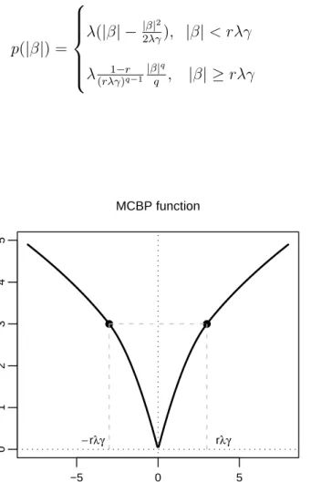
p(|β|) = λ(|β| − |β|2λγ2), |β|< rλγ λ(rλγ1−r)q−1 |β|q q , |β| ≥rλγ (4.1) −5 0 5 0 1 2 3 4 5 ● ● rλγ −rλγ β p ( β ) MCBP function
Figure 4.1: Minimax Concave Bridge Penalty function, γ = 3, r = 2/3
We observe that forp(|β|) to be continuous at the knot rλγ, we require, λ(rλγ− (rλγ) 2 2λγ ) = λ 1−r (rλγ)q−1 (rλγ)q q which reduces to r−r 2 2 = r(1−r) q and thus q= 2− 2 2−r = 2(1−r) 2−r With this relationship between q and r, we observe that
1. we have the MCP penalty function when r→1, and 2. we have the L1 penalty function whenr →0.
This is expected based on the construction of the MCBP function. This shows that our penalty function is indeed more general with the Lasso and the MCP as special cases.
We would like to highlight that the MCBP function is developed with implementation and computation in mind. The number of tuning parameters that need to be estimated is kept to the minimum. The MCBP function is made continuous at the single knot by simply establishing a relationship between r and q rather than by a translation of the derivative via an arbitrary constant. In this manner, though we have inevitably compro-mised in terms of a wider spectrum of penalty function, we have gained in the need to estimate a larger number of tuning parameters.
The penalized likelihood with the MCBP function for the generalized linear model is therefore min β − 1 n n X i=1 logfi(g(xTi β),yi) + d X j=1 p(|βj|) (4.2)
where yi has a densityfi(g(xTi β),yi)) and g is the inverse link function.
Particularly, the penalized likelihood with the MCBP function that will address data with multinomial dependent response and possibly separation is as follows:
min β − 1 n n X i=1 [yi(xTi β)−log[1 + exp(xTi β)]] + d X j=1 p(|βj|) (4.3)
4.4
Properties and Justifications
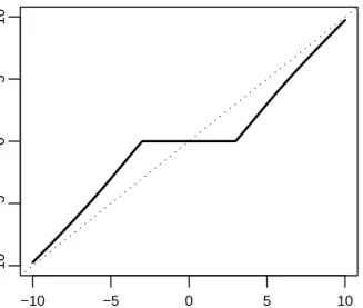
The plot of the sum of|β| and the derivative of MCBP function is as follows:
−5 0 5 0 2 4 6 8 ● ● rλγ −rλγ β Figure 4.2: Plot of |β|+p0(|β|)
From the plot, it is not difficult to see that MCBP function satisfies the conditions for sparsity and continuity as laid out by Fan and Li [17]. The MCBP function has a singularity at zero and therefore has the important property of sparsity, a much desired property for model selection with high dimensional data. Unlike the bridge penalty function which does not have the continuity property despite having oracle property, a much lamented deficiency highlighted by Zou [59], MCBP function, with γ > 1, has the continuity property and is able to provide a “smooth” transition from one plausible model to another. The unbiasedness property is inferred from the work done by Knight and Fu as well as Huang et.al..
−10 −5 0 5 10 −10 −5 0 5 10 β ^ βOLS
Penalised least square estimators
Figure 4.3: PLS estimator or thresholding rule of MCBP function
be unlike L1 and will not over penalize true parameters that are large. At the same
time, unlike SCAD or MCP, the MCBP function will not under-penalize untrue large pa-rameters that arise from situation with separation. Hence, MCBP function is a penalty function that possesses the desired properties in model selection and is able to address the issue of separation. Separately, MCBP function, though non-convex, is explicit in form and its asymptotic properties can be examined analytically when compared to methods featured in Chapter 3.
Finally, MCBP function can be perceived as a versatile penalty function. With suit-able choice ofr, it can be the Lasso penalty function or the MCP penalty function or in between. An algorithm developed for the implementation of this penalty function will enable a one-stop analysis without the need to switch fromLARs for Lasso to PLUS or ncvreg for MCP.
In the next chapter, we develop the computational algorithm for the implementation of the MCBP function.
Computation
In Chapter 4, we have justified that the Minimax Concave Bridge Penalty function has all the desired properties in model selection as well as the capability to resolve separation in data. It is, however, a nonconvex penalty function. Practitioners have been lukewarm in embracing methods that have nonconvex objective functions due to the numerical challenges in optimizing and the often unstable solutions. In studies involving high dimensionality, it is inevitable that practitioners factor computational efficiency as part of the equation to decide on the approach to the analysis. As such, to complete our proposal, we will provide a matching efficient computation algorithm that befits the theoretical attractiveness of the MCBP function and one which will facilitate the fitting of MCBP models.
5.1
Some methods on non-convex optimization
In Chapter 2, we observed that a necessary condition for penalty functions to possess the desired properties of model selection is to be nonconvex. SCAD and MCP are two examples of such nonconvex penalty functions and numerous computation algorithms
5.1.1
Local Quadratic Approximation
Fan and Li, in their introduction to the SCAD penalty function, proposed to locally approximate penalty functions that are singular at the origin and do not have a continuous second order derivative with a quadratic function. In particular, supposeβ(0) is an initial value that is close to the true value ofβ, Fan and Li proposed locally approximating the first order derivative of the penalty function by a linear function:
[pλ(|βj|)]0 =p0λ(|βj|)sgn(βj)≈
[p0(|βj(0)|)
|βj(0)|] βj forβj(0) 6= 0.
This linear approximation of the first order derivative leads to a local quadratic ap-proximation (LQA) of the penalty function:
pλ(|βj|)≈pλ(|β (0) j |) + 1 2{ p0λ|βj(0)|) |βj(0)| }(β 2 j −β (0)2 j ).
A modified Newton-Raphson algorithm is subsequently applied to optimize this ap-proximated penalized likelihood. Specifically, using the unpenalized maximum likelihood asβ(0), we solve iteratively β(m+1) = arg min{−1 n n X i=1 li(β) + d X j=1 p0λ(|βj(m)|) 2|βj(m)| β 2 j} till β(n) converges.
This algorithm, however, has a similar drawback to stepwise variable selections. A covariate that is being removed during the LQA algorithm will not be included in the final selected model [17]. Hunter and Li [31] managed to alleviate this issue by optimizing a slightly perturbed version of the LQA but the size of perturbation to adopt remains unanswered. Fan and Li [17] suggested using the one-step (ork-step) estimate from the iterative LQA algorithm with good starting estimators to overcome the computational difficulty but such an approach cannot have sparse representation and this runs against the desired property of the nonconvex penalty function.
5.1.2
Local Linear Approximation
Zou and Li [61] proposed a unified algorithm to solve nonconvex penalized likelihood based on locally linearly approximating (LLA) the penalty function. That is,
pλ(|βj|)≈pλ(|βj(0)|) +p 0 λ(|β (0) j |)(|βj| − |βj(0)|) forβj ≈β (0) j .
Similar to the LQA algorithm, the maximization of the penalized likelihood can be solved iteratively using
β(m+1) = arg min{−1 n n X i=1 li(β) + d X j=1 p0λ(|βj(m)|)|βj|}
with the unpenalized maximum likelihood estimate, β(0), used as the initial value till β(n) converges.
com-coefficient to avoid numerical instability and is shown to be the best convex minoriza-tion maximizaminoriza-tion (MM) algorithm [61]. The convergence of the LLA algorithm is also assured by the ascent property of MM algorithm [35]. The LLA algorithm inherits the good features of LASSO in terms of computational efficiency and can therefore ride on the many algorithms developed for Lasso such as least angle regression (LARs) [16].
Both the LQA and LLA are just some of the numerous computational algorithms that estimate parameters of nonconvex penalized likelihood. One assumption made in these algorithms is a good inital estimate,β(0), in the vicinity of the trueβ. Both LQA and LLA suggested the use of the unpenalized MLE as the initial value. In data with separation, however, MLE does not exist and this limits the utility of these approaches. In addition, this also implicitly assumes thatd << nand therefore these methods are not applicable in situations when d is larger than n. Furthermore, these methods optimize the penalized likelihood discretely and do not provide a whole solution path and will be a challenge to implement when high-dimensional data is involved.
Many other similar methods that approximate the nonconvex penalty function with a convex penalty function followed by iterative application of convex optimization al-gorithm to arrive at an estimate have been developed. Separately, Breheny and Huang [9] proposed to apply the coordinate descent algorithms to SCAD and MCP regression models and have made ncvreg , the algorithm in R package, available for use.