Robust Model Selection in Dynamic Models with an Application to Comparing Predictive Accuracy

(1)

CAE Working Paper #06-09

Robust Model Selection in Dynamic Models with an

Application to Comparing Predictive Accuracy

by

Hwan-sik Choi

and

Nicholas M. Kiefer

September 2006

.

(2)

Robust model selection in dynamic models with an

application to comparing predictive accuracy

Hwan-sik Choi

∗

Cornell University

Nicholas M. Kiefer

†

Cornell University

September, 2006

Abstract

A model selection procedure based on a general criterion function, with an example of the Kullback-Leibler Information Criterion (KLIC) using quasi-likelihood functions, is considered for dynamic non-nested models. We propose a robust test which generalizes Lien and Vuong’s (1987) test with a Heteroscadasticity/Autocorrelation Consistent (HAC) variance estimator. We use the fixed-b asymptotics developed in Kiefer and Vogelsang (2005) to improve the asymp-totic approximation to the sampling distribution of the test statistic. The fixed-b approach is compared with a bootstrap method and the standard normal approximation in Monte Carlo simulations. The fixed-b asymptotics and the bootstrap method are found to be markedly superior to the standard normal approximation. An empirical application for foreign exchange rate forecasting models is presented.

JEL classification: C12, C14, C15, C52

Keywords: Kullback-Leibler Information Criterion (KLIC), quasi-likelihood, dynamic models, fixed-b asymptotics, bootstrap method, Monte Carlo simulation. ∗_{[email protected]. 404 Uris Hall, Department of Economics, Cornell University, Ithaca, NY, 14850, USA.} †_{[email protected]. 490 Uris Hall, Department of Economics and Department of Statistical Science, Cornell}

(3)

1 Introduction

Since Cox (1961, 1962), many methods for distinguishing separate families of hypotheses for model selection have been developed. Model selection is quite different from nested hypothesis testing. The null hypothesis in nested hypothesis testing is well defined but the alternative hypothesis can be arbitrarily close to, though different from, the null, and therefore difficult to detect. Further, these close alternatives may not be importantly different from the null in any practical sense. In contrast, non-nested hypothesis testing has clear separation between candidate models but presents the difficulty of choosing a sensible null hypothesis. Cox used centered log likelihood ratios between two nested models under the null hypothesis that one of the models is true. A test for non-nested linear regression models was developed in Pesaran (1974). Along the tradition of the nesting approach of Atkinson (1970) which sets up a general model that contains the candidate models, the_J test of Davidson and MacKinnon (1981) is popular (McAleer (1995)). See Gourieroux and Monfort (1999) for a summary.

There is a different approach that does not assume the true model is among the candidates. Vuong (1989) considered a selection criterion based on the difference in the Kullback-Leibler In-formation Criterion (KLIC, Kullback and Leibler (1951)) between the (unknown) true model and the competing models, and the null hypothesis is that two models are equivalent in KLIC. This approach has the advantage of treating two competing models symmetrically and it does not re-quire the specification of a nesting model. Vuong’s approach is sometimes calledmodel selection in contrast to non-nested hypothesis testing (Davidson and MacKinnon (2004)). It has recently been extended for dynamic models using different criterion functions (see Rivers and Vuong (2002)).

In non-nested hypothesis testing, the usual asymptotic approximation to the distribution of the J test statistic is known to be poor even with large samples (Godfrey and Pesaran (1983), McAleer (1995)) and the bootstrap is an attractive alternative in these cases (see Fan and Li (1995), Godfrey (1998), Davidson and MacKinnon (2002), and Choi and Kiefer (2005)). But in model selection, less is known about the performance of the asymptotic approximations of the Vuong (1989) and Rivers and Vuong (2002) test.

(4)

This paper proposes a generalized model selection test for dynamic models using a Heteroscadas-ticity/Autocorrelation Consistent (HAC) estimator of the long run variance as in Rivers and Vuong (2002), and using Kiefer-Vogelsang-Bunzel (KVB) fixed-b asymptotics (Kiefer, Vogelsang, and Bun-zel (2000), Kiefer and Vogelsang (2002a,b, 2005)) to approximate the finite sample distribution of our test statistic. Our approach is applicable to general criterion functions and robust to un-known (nonparametric) serial correlation in the data. Specifically, we represent the idea using a model selection criterion based on quasi-likelihood functions and the resulting test statistic forms a difference-in-KLIC measure. Many general criterion functions can be interpreted as quasi-likelihood functions. The quasi-likelihood functions were used for Monte Carlo study of performance of our test statistic. Our method is compared with a bootstrap method and the conventional standard normal approximation and shown to be remarkably superior to the standard normal approximation. We also considered a prediction accuracy measure for an empirical application. Our approach was used for two competing exchange rate forecasting models. In the forecasting model comparison literature, a bootstrap method is also used by White (2000). White considers a “benchmark” model and a group of alternative models. The null is that none of the other models dominates the benchmark. The differences between the forecast errors from the benchmark model and all alternatives are arranged in a vector. Then, the test is that the maximum of these differences is negative, so no model dominates the benchmark. The distribution of this maximum is obtained by the stationary bootstrap of Politis and Romano (1994). Thus, this test is like ours, but the null is different, favoring a benchmark model, and of course there is no HAC estimator or fixed-b approximation. Hansen (2005b) also considers comparing a benchmark model with a number of alternatives. He tests the superiority of the benchmark model and uses the stationary bootstrap methods as in White (2000). Hansen (2005b) differs from White (2000) in that he studentizes the statistic before taking the maximum. White is essentially using the null that is closest to the alternative. Hansen estimates the null mean, rather than using zero.

Instead of testing a superiority of prediction accuracy, the idea of testing equivalence in a criterion function is used in Diebold and Mariano (1995) (DM test). The DM test compares forecast accuracy of two competing models, where the accuracy is measured by some criterion function (such

(5)

as a goodness of fit measure) and the null is that the forecasts are equally accurate. It is similar to Vuong (1989), except the likelihood is not used, rather a fairly general function of the fit. The variance estimator in the DM test is also a HAC estimator. Harvey, Leybourne, and Newbold (1997) attempted to improve finite sample performance of the DM test by using a correction factor to the DM test statistic (MDM (Modified DM) test).

Our approach is applicable to the DM test. An empirical application for the DM test is presented for testing equality of predictive accuracy of the foreign exchange rate forecasting models considered in Diebold and Mariano (1995) using USD/EURO and YEN/USD exchange rate data. Although we aim to improve the ﬁnite sample properties of the DM test statistic, our approach is diﬀerent from the MDM test in two aspects. First, our test considers a better approximation to the whole distribution of the test statistic whereas the MDM test considers thescaled normal approximations only. Second, our approximation depends on the kernel function and bandwidth used in a HAC estimator whereas MDM is derived for a particular kernel function (the uniform kernel) and a bandwidth (a forecasting horizon) used in the DM test.

2 KVB fixed-b asymptotics

HAC variance estimators are used frequently in econometrics for test statistics involving serially correlated observations. The standard (normal) approximation to the sampling distributions of HAC estimators assumes that the long-run variance is known and equal to its estimated value. The resulting distribution does not depend on the kernel or bandwidth used in variance estimation and is known to give a poor approximation to the sampling distribution, especially for size calcula-tion. Kiefer, Vogelsang, and Bunzel (2000), Kiefer and Vogelsang (2002a,b, 2005) proposed a new asymptotic approximation to the sampling distribution of HAC estimator (and test statistic). They proposed to generate the approximate distribution by fixing theratio _M/T =_{b >}0 as _T goes to infinity. (In the conventional approach,_b converges to zero.) Under this new set-up, the limit of HAC estimator does not converge to the long-run variance but to the long-run variance multiplied by a functional of aBrownian bridge. This approach is called the ‘fixed-b’ approach in comparison

(6)

to the conventional ‘small-b’ approach.

Let_V_T be a HAC estimator (used in the denominator of a test statistic) given by

VT = T−1 j=1−T K j M ˆ γ(_j)_, (2.1)

where_K(_x) is the kernel with support [−1_,1],_T is the sample size,_M is the number of lags or the truncation number, and

ˆ γ(_j) = 1 T T t=j+1 (ˆ_u_t−_u¯)(ˆ_u_t₋_j−¯_u)_, (2.2) where{_uˆ_t}is the estimated values of the stochastic process of interest, for example, residuals, scores, or other criteria used in a test statistic, and ¯_uis the sample mean of ˆ_u_t (Often we have ¯_u= 0 as in residuals from linear regression with a constant term or scores). The limiting distribution of_V_T under the ﬁxed-b asymptotics assumption _M/T = _b as _T → ∞ depends on the kernel function K(_x) and the bandwidth_b.When the functional central limit theorem (FCLT) holds for the partial sum, i.e. T−1/2 [rT] t=1 ut⇒λW(r), (2.3)

where_λ2=∞_j₌_−∞_γ(_j) and_W(_r) is the standard Brownian motion deﬁned on_C[0_,1], and when the Bartlett (triangular) kernel is used, we have

VT ⇒ 2_λ2 b 1 0 W (_r)2 _dr− ₁₋_b 0 W (_r+_b)_W(_r)_dr , (2.4)

where_W(_r) is aBrownian bridge deﬁned as_W(_r) =_W(_r)−_rW(1)_,under the assumption_M/T = b >0 as_T → ∞. In testing applications, _λ2 is cancelled out with the asymptotic variance of the numerator of a test statistic making the test statistic pivotal.

Conditions for the FCLT are slightly weaker than the assumptions required for the consistency of HAC estimator. A discussion of the assumptions imposed for the FCLT is given in Kiefer and Vogelsang (2005). Cases with diﬀerent kernel functions are also in Kiefer and Vogelsang (2005). A simple example is in Choi and Kiefer (2005). We assume a FCLT applies to the related partial

(7)

sums in this paper.

3 Dynamic Model Selection Testing

3.1 The test statistic and limiting distributions

Let _p₁(_z₁_{, θ}₁) and _p₂(_z₂_{, θ}₂) be two models to compare, and (_z_i_{, θ}_i) are the variables and the parameter vector used in the model_i= 1_,2_.

Assumption 3.1 The stochastic process_z_i={_z_it}∞_t₌_−∞ is weakly stationary for _i= 1_,2.

We consider{_z₁_t_{, z}₂_t}T

t=1 are the available data used for the model comparison (and estimation of the parameter vectors).

Assumption 3.2 For _i= 1_,2, the estimator _θˆ_i of _θ_i converges to a fixed vector _θ∗_i in probability, i.e.

ˆ

θi→p θi∗. (3.1.1)

The limits _θ∗_i (_i = 1_,2) are called pseudo-true values when the models are misspeciﬁed. This high-level assumption can itself be based on assumptions about the objective function (for example identiﬁcation) and the parameter space (for example compactness in the case of an extremum esti-mator). We assume 3.2 directly, noting that there are many routes to the result such as (quasi) max-imum likelihood estimation (MLE), generalized method of moments (GMM), minmax-imum divergence estimators (MDE), generalized empirical likelihood (GEL), and other parametric, semiparametric methods.

We consider a model selection procedure that compares_Q_i (of a criterion function) from model i= 1_,2, then chooses the model that has the smallest_Q_i_.We assume that_Q_i satisﬁes the following assumption.

Assumption 3.3 (Weak law of large numbers) Let the value of the model selection criterion at pseudo-true values _θ∗_i be _Q_i = _Q_i(_z_i_{, θ}_i∗) for models _i = 1_,2_. We have a function _Q_iT =

(8)

QiT({zit}Tt=1,θˆi) of the data available that satisfies Qi= plim T→∞ QiT. (3.1.2) Denoting_QT_it=_Q_i(_t,{_z_is}T_s₌₁_,_θˆ_i)_, we have plim T→∞ T t=1 QTit/T p →Qi,

and when_Q₁=_Q₂, we also have an approximation of√_T(_Q₂_T −_Q₁_T)given by √ T(_Q₂_T −_Q₁_T)− T t=1 (_QT₂_t−_QT₁_t)_/√_T p →0_. (3.1.3)

Assumption 3.3 allows us to calculate the asymptotic variance of (_Q₂_T −_Q₁_T) using {_QT₂_t−

QT1t}Tt=1 under Q1=_Q₂. This assumption is satisﬁed in many model selection criterion including lack of ﬁt measures such as the mean squared error (_QT

it = (yit−yˆit)2) or mean absolute error (_QT

it = |yit−yˆit|). When the criterion function is a quasi-likelihood, we use ﬁrst order Taylor expansion of_Q_iT = ln ˆ_σ2_i around the pseudo-true value (_σ∗_i)2 and get

QTit= ln(_σ∗_i)2+ uˆ 2 it (_σ_i∗)2 −1 , (3.1.4)

where ˆ_σ_i2 = T_t₌₁_uˆ2_it_/T and ˆ_u_it are residuals from the quasi-maximum likelihood estimation (QMLE) of the models_i= 1_,2. This approach was used in Lien and Vuong (1987).

We introduce an additional assumption on _QT_it for asymptotic approximation of the sampling distribution of our test statistic to be described later.

Assumption 3.4 (Functional Central Limit Theorem) Let {_vˆ_t}T

t=1 = {QT2t−QT1t}Tt=1. We have T−1/2 [rT] t=1 ˆ vt⇒λW(r), (3.1.5)

(9)

{_vˆ_t}.

Assumption 3.4 holds under a variety of regularity conditions and permits conditional het-eroscadasticity in {_vˆ_t} but rules out most form of unconditional heteroscadasticity. A set of suffi-cient conditions can be found in Phillips and Durlauf (1986) which require that the process{_vˆ_t}is weakly stationary, satisfies_α-mixing conditions, and each element ˆ_v_t has a finite moment greater than two. The condition holds for stationary and invertible ARMA processes with innovations with finite fourth moments (Hall and Heyde (1980), see Kiefer, Vogelsang, and Bunzel (2000) for further discussion).

Our null hypothesis is that the competing models are asymptotically “equal”, i.e.

Q1−Q2= 0, (3.1.6)

and the test statistic is given by

τT = _T t=1(QT2t−QT1t)/ √ T VT , (3.1.7)

where_V_T is the HAC variance estimator of the serially correlated process{ˆ_v_t}={_QT

2t−QT1t}given by VT = T−1 j=1−T K j M ˆ γ(_j)_, (3.1.8)

where _K(_x) is the kernel function, _M is the bandwidth used in the kernel estimation and the autocovariance function estimator ˆ_γ(_j) is given by

ˆ γ(_j) = 1 T T t=j+1 (ˆ_v_t−_v¯)(ˆ_v_t₋_j−_v¯)_, (3.1.9) where ¯ v= 1 T T t=1 ˆ vt. (3.1.10)

(10)

This approach does not specify a correct model and treats two competing models symmetrically. Also it is directional, under an alternative, favoring the model 1 when_τ_T a.s.→ +∞ and vice versa, if we exclude the cases where_Q_i is not deﬁned under the alternative.

Theorem 3.5 Under the assumption 3.1−3.4, the limiting distribution of the test statistic_τ_T under

M/T →b >0 is given by the KVB fixed-b asymptotics_. For example, with the Bartlett kernel and for a bandwidth_M/T →_b∈(0_,1]_,we have

τT −→d N(0_,1) 2 b ₁ 0 W(r)2 dr− ₁₋b 0 W(r+b)W(r) dr . (3.1.11)

Proof. The result directly follows from Theorem 1 in Kiefer and Vogelsang (2005).

Diﬀerent kernels give diﬀerent denominators in the limiting distribution, thus our approximating distribution depends both on the kernel and bandwidths used.

3.2 Quasi-likelihood criterion

In general, the selection criterion_Q_i should also be the objective function used in estimation, but this is not necessary. See Rivers and Vuong (2002) for a discussion of using a different model selection criterion than the estimation criterion. See also Pötscher (1991) and Hansen (2005a) for how a model selection step can affect the inference for the models.

We consider the quasi-likelihood function for both the estimation and selection criteria as an example (Many other estimation methods have QMLE interpretation). The quasi-likelihood we specify is the likelihood under normality with independent observations (Heyde (1997)). The quasi-likelihood method leads to consistent parameter estimation under certain conditions (for example, OLS with exogenous regressors and serially correlated errors is consistent). When it is not con-sistent, its probability limits are pseudo-true values. Using quasi-likelihood also gives our model selection criterion a KLIC interpretation. See Vuong (1989).

(11)

quasi-log likelihood ratio ln_p₁(ˆ_θ₁)−ln_p₂(ˆ_θ₂) =T 2 ln(ˆσ 2 2/σˆ12), (3.2.1) and given by τT = √ Tln(ˆ_σ2₂_/ˆ_σ₁2) VT , (3.2.2)

The HAC variance estimator_V_T for ˆ vt=QT2t−QT1t (3.2.3) = ln(_σ∗₂)2−ln(_σ∗₁)2+ uˆ 2 2t (_σ₂∗)2 − ˆ u21t (_σ₁∗)2 , (3.2.4)

is given by plugging ˆ_v_t into eq. (3.1.9) and using the estimated ˆ_σ2_i for (_σ∗_i)2 in eq. (3.2.4). The sampling distribution of the test statistic_τ_T is approximated by diﬀerent ﬁxed-b asymptotic ap-proximations depending on the kernel function and the bandwidth.

If the data are i.i.d., this test can be implemented easily (see Lien and Vuong (1987) and Vuong (1989)). Our approach is similar to Lien and Vuong (1987), but we consider serial correlation in ˆ

vt.Our approach includes Lien and Vuong (1987) as a special caseM = 1. It should be noted that our quasi-likelihood function is applicable to nonlinear models, and our approach in general can be used for any model selection criteria satisfying the assumption 3.3 such as the lack of fit criterion, mean squared prediction error (used in Rivers and Vuong (2002)) or mean absolute error (used in Diebold and Mariano (1995)). Our test statistic is also similar to the one considered in Rivers and Vuong (2002). But we use a different approximate distribution given by the KVB approach. We use the quasi-likelihood criterion and show by Monte Carlo simulations that the KVB fixed-b approach gives a superior approximation to the standard normal approximation based on the usual HAC asymptotics.

(12)

3.3 The bootstrap method

Bootstrap methods are popular alternatives to the conventional asymptotic approximation in econo-metrics. In the non-nested hypothesis context, the bootstrap is known to improve the approximation of the sampling distributions of test statistics. See Fan and Li (1995), Godfrey (1998), Davidson and MacKinnon (2002), and Choi and Kiefer (2005).

We used a bootstrap method for our test statistic in a similar way to the method in Hall and Horowitz (1996) and White (2000). In the fixed-b asymptotics, the leading term in the asymptotic expansion is not normal, and the validity of the bootstrap is an open question. Recently, Gon¸calves and Vogelsang (2006) showed that the “naive” block bootstrap has the same limiting distribution as the fixed-b asymptotics. The argument proceeds by writing the test statistic and the bootstrap test statistic as the same functions of the data and the bootstrap data respectively. Using appropriate assumptions on the bootstrap data and the continuous mapping theorem gives the result that the limit distributions are identical. Showing that the resulting distribution is an improvement on the normal approximation is more difficult. Gon¸calves and Vogelsang (2006) are able to obtain this result for a special case (estimation of a normal mean). See also Jansson (2004) who shows that the fixed-b asymptotics can improve on the normal approximation in terms of rate of error in rejection probability (ERP). Our simulation results indicate that the bootstrap is practically useful in our settings.

Our null hypothesis does not assume a speciﬁc form of the true model, therefore we can not use the explanatory variables as given and generate bootstrap samples. This implies that since neither of the candidate models is correct, we should not bootstrap from one particular model. Instead, we should bootstrap from the joint empirical distribution of the dependent variable and the explanatory variables (sampling together (_y_t_{, x}_t) for example). Consequently, when the bootstrap samples are drawn from the original samples which may happen to be a realization in favor of one model over the other, the distribution of the bootstrap test statistic will be biased and give inaccurate critical values. This happens because it is hard to implement the null hypothesis in generating bootstrap samples in our setting. We correct the bootstrap test statistics using the statistics from the original

(13)

sample as standard in bootstrap literature. We use the quasi-likelihood criterion and the bootstrap test statistics is given by

tb= √ Tln(˜_σ2₂_/˜_σ₁2)−_C₀ VT , (3.3.1)

where ˜_σ₁2 and ˜_σ₂2are the variance estimators calculated with the bootstrap samples, and

C0= lnσˆ 2 2 ˆ

σ2₁, (3.3.2)

where ˆ_σ₁2 and ˆ_σ₂2 are variance estimators from the original sample, and _V_T is calculated from eq. (3.1.8) and (3.1.9) with ˜ vt= ˜ u22t ˆ σ22 − ˜ u21t ˆ σ21 −D1 , (3.3.3) where D1= σ˜ 2 2 ˆ σ22 − ˜ σ21 ˆ σ21. (3.3.4)

We have applied the bootstrap method to our examples in the simulation section of this paper. Direct (without modiﬁcation) bootstrap is not recommended in any case. For all examples, we considered block bootstraps with the block sizes one (the i.i.d. bootstrap) and ﬁve.

We also emphasize that a special concern is required for the candidate models with lagged variables. Since the bootstrap cannot be semi-parametric for the nature of the problem, it is hard to generate the bootstrap {_y_t} sequentially. We propose to use non-parametric bootstrap with

{yt, yt−j, xt}, where yt−j is the vector of all the lagged variable used as explanatory variables in the candidate models and_x_t is the vector of all the other explanatory variables, and we drop the ﬁrst_J observation where_J is the highest lagged number used. We used this method for our MA(2) example later in this paper.

(14)

3.4 Linear models: A Curious Result

We consider a special case in which the true model is linear when the quasi-likelihood criterion is used. The true model is

yt=wtδ+xtα1+ztα2+ut(t= 1, ..., T), (3.4.1)

where{_u_t}is a mean zero weakly stationary process with autocovariance function_γ(_j)_,and_w_t_{, x}_t_{, z}_t are weakly stationary and correlated each other. The competing models are

H1:_y_t=_w_t_δ₁+_x_t_β₁+_u₁_t_, (3.4.2)

H2:yt=wtδ2+ztβ2+u2t, (3.4.3)

where_t= 1_{, ..., T} (_T is the number of observations),_w_tis the (_l×1) vector of common regressors, and_x_t,_z_tare (_k₁×1) and (_k₂×1) explanatory variables respectively. The parameters (_δ_i_{, β}_i_{, σ}_i2) are conditional mean and variance parameter vectors for model_H_i. As typical for economic data, wt, xtandztare serially correlated and the unknown true model’s errors are also serially correlated. We rule out data generating processes (DGPs) for which the models_H₁and_H₂are identical (_δ₁=_δ₂ and_β₁=_β₂= 0 for our example), as in this case there is no real testing problem. Let (_δ∗₁_{, δ}₂∗) be the pseudo true values of (_δ₁_{, δ}₂) and (_β₁∗_{, β}₂∗) be the pseudo true values of (_β₁_{, β}₂)_.

Assumption 3.6 With _ξ_t= (_w_t_{, x}_t_{, z}_t)_,two processes, {_u_t} and{_ξ_t}_,are independent.

Assumption 3.7 The regressors _w_t_{, x}_t_, and _z_t are serially uncorrelated but possibly correlated contemporaneously.

Assumption 3.8 Two competing models are equal in quasi-likelihood criterion from the true model, i.e. plim_σˆ₁2=plim_σˆ2₂_.

We have the following theorem under the above assumptions.

Theorem 3.9 Under assumptions 3.6, 3.7 and 3.8, the autocovariance function Cov(_U_t_{, U}_t₋_j)of

(15)

Proof. We have Ut=u22t−u21t = (_y_t−_w_t_δ₂∗−_z_t_β∗₂)2−(_y_t−_w_t_δ₁∗−_x_t_β₁∗)2 ={_w_t(_δ₁∗−_δ∗₂) +_x_t_β₁∗−_z_t_β₂∗}[2_y_t− {_w_t(_δ∗₁+_δ∗₂) +_x_t_β∗₁+_z_t_β₂∗}] ={_w_t(_δ₁∗−_δ∗₂) +_x_t_β₁∗−_z_t_β₂∗}[2 (_u_t+_w_t_δ+_x_t_α₁+_z_t_α₂)− {_w_t(_δ₁∗+_δ∗₂) +_x_t_β∗₁+_z_t_β₂∗}] ={_w_t(_δ₁∗−_δ∗₂) +_x_t_β₁∗−_z_t_β₂∗}[2_u_t+_w_t{2_δ−(_δ∗₁+_δ₂∗)}+_x_t(2_α₁−_β₁∗) +_z_t(2_α₂−_β₂∗)] = 2_u_t{_w_t(_δ₁∗−_δ∗₂) +_x_t_β₁∗−_z_t_β₂∗} +{_w_t(_δ₁∗−_δ₂∗) +_x_t_β∗₁−_z_t_β₂∗}[_w_t{2_δ−(_δ₁∗+_δ∗₂)}+_x_t(2_α₁−_β₁∗) +_z_t(2_α₂−_β₂∗)]_. Under assumption 3.8 we have

E(_U_t) = 0_, therefore Cov(_U_t_{, U}_t₋_j) =_E(_U_t_{, U}_t₋_j)_. If we put At={wt(δ∗1−δ2∗) +xtβ1∗−ztβ2∗}, Bt={wt(δ∗1−δ2∗) +xtβ1∗−ztβ2∗}[wt{2δ−(δ∗1+δ2∗)}+xt(2β1−β∗1) +zt(2β2−β2∗)], we have E(_U_t_{, U}_t₋_j) =_E(2_u_t_A_t+_B_t) (2_u_t₋_j_A_t₋_j+_B_t₋_j) = 4_E(_u_t_u_t₋_j_A_t_A_t₋_j) +_E(_B_t_B_t₋_j) = 4_γ(_j)_γ_A(_j) +_γ_B(_j)_, (3.4.4)

(16)

from the independence between_u_tand_A_tby the assumption 3.6. Assumption 3.7 implies_γ_A(_j) = 0 and_γ_B(_j) = 0 for all_j = 0. Therefore we have_Cov(_U_t_{, U}_t₋_j) = 0 for_j= 0_.

Theorem 3.9 implies that under the assumptions 3.6 and 3.8, autocorrelation in_u_tdoes not aﬀect the asymptotic variance of the numerator of our statistic unless the regressors are autocorrelated. The Monte Carlo simulations supported this.

3.5 Power of the test

For the comparison of two different test statistics, size corrected power is often used. Since we have proposed different approximations to the distribution of the same test statistic, size corrected power comparisons are not applicable. To check the finite sample power properties of the fixed-b approximation, we did the following experiments.

• For different sample sizes, compare the powers as a function of the levels implied by the fixed-b approximating distrifixed-butions given a fixed alternative, a kernel function, and a fixed-bandwidth. We considered_T = 50_, 100_, 200.

• For the diﬀerent sample sizes, compare the local powers given a level, a kernel function, and a bandwidth.

• For different kernel functions, compare the local powers given a level, a bandwidth, and a sample size. We considered five different kernels, Bartlett, Parzen, Quadratic spectral, Daniell, and Bohman. In the fixed-b approach, different kernels give different approximating distributions. We calculated the critical values using the formula given in Kiefer and Vogelsang (2005) for each kernel.

Note that the asymptotic power was not available for the traditional standard normal approx-imation, since the test statistic’s (traditional) limiting distribution under the local alternative is identical regardless of the choice of kernels and bandwidths. The fixed-b asymptotics makes possi-ble comparison of the asymptotic powers for different kernels and bandwidths as shown in Kiefer and Vogelsang (2005). Our finite sample power comparison showed that the fixed-b asymptotic

(17)

power comparison can be useful in understanding the actual difference in the finite sample powers among kernels and bandwidth choices. The simulation in the next section showed that the fixed-b approximation has reasonable power.

4 Monte Carlo Study

We consider two data generating processes. An MA(2) model, and linear regression with autocor-related regressors and errors.

4.1 Size Comparison

4.1.1 MA(2) model

Consider the following MA(2) true data generating process

yt=εt+ 0.5εt−1+εt−2 (t= 1, ..., T), (4.1.1)

where_ε_t∼i.i.d._N(0_,1)_.The competing models are AR models

H1:yt=α1+βyt−1+ε1t, (4.1.2)

H2:_y_t=_α₂+_δy_t₋₂+_ε₂_t_, (4.1.3)

where_ε₁_t and _ε₂_tare assumed to be white noises. The true model has _γ(1) =_γ(2), and we know ˆ

β−→p γ(1)_/γ(0) and ˆ_δ−→p _γ(2)_/γ(0)_.Thus we have the same pseudo true values,_β∗=_δ∗. From this fact we can easily show

plim ˆ_σ2₁= plim ˆ_σ₂2_, (4.1.4)

which implies they are equivalent in our quasi-log likelihood criterion function. The variance ˆ_σ2₁ and ˆ_σ₂2were calculated based on_T−1 observations in_H₁and_T−2 observations in_H₂respectively, and the HAC denominator was based on_T−2 residuals from_H₁and_H₂(we dropped out the ﬁrst

(18)

residual from_H₁)_.The test statistic is given by τT = √ T−2 lnˆ_σ₂2_/_σˆ₁2 VT . (4.1.5)

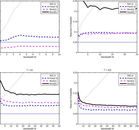
The number of iteration of the simulation was 5_,000. We used four sample sizes_T = 12_,27_,52_,102 for the convenience of the bootstrap. The test are 5% level two tail tests. For the bootstrap tests, we resampled the lagged variables {_y_t_{, y}_t₋₁_{, y}_t₋₂} together, dropping the first two observations. Therefore the bootstrap sample size is_T−2, and our choice of sample sizes makes the block bootstrap simple. We used two different block sizes, one (the i.i.d. bootstrap) and five. Of course the i.i.d. bootstrap ignores the serial dependence in the data. The bootstrap critical values were obtained from the 2.5% and 97.5% quantiles of the empirical distribution of the 1_,200 bootstrap iterations. The empirical rejection rates of the standard normal, fixed-b, i.i.d. bootstrap (‘boot(1)’),and block bootstrap (‘boot(5)’) are shown in Figure 1.

The fixed-b asymptotics showed great improvement upon the standard normal approximation especially when a large_M is used for all sample sizes considered. Also the i.i.d. bootstrap approach was better than the block bootstrap and similar to, but a little bit worse than, the fixed-b approx-imation. For large sample sizes (_T = 52_,102) the block bootstrap improves, but in all cases the fixed-b approximation was better than the others. We surmise that a more sophisticated bootstrap approach is required in this setting.

4.1.2 Linear regression model

We generated the following variables for_t= 1_{, ..., T}

ut=αut−1+εt, εt∼i.i.d.N (0,1), (4.1.6)

wt=ρwt−1+ζ1t, (4.1.7)

xt=ρxt−1+ζ2t, (4.1.8)

(19)

and _⎛ ⎜ ⎜ ⎜ ⎜ ⎝ ζ1t ζ2t ζ3t ⎞ ⎟ ⎟ ⎟ ⎟ ⎠∼i.i.d. N ⎛ ⎜ ⎜ ⎜ ⎜ ⎝0, ⎡ ⎢ ⎢ ⎢ ⎢ ⎣ 1 _κ₁ _κ₁ κ1 1 _κ₂ κ1 κ2 1 ⎤ ⎥ ⎥ ⎥ ⎥ ⎦ ⎞ ⎟ ⎟ ⎟ ⎟ ⎠, (4.1.10)

where_{α, ρ, κ}₁_{, κ}₂are parameters we choose for the simulation. We consider two cases as true models

Case I :_y_t=_w_t+ 0_.5_x_t+ 0_.5_z_t+_u_t_, (4.1.11)

Case II :_y_t=_w_t+ 0_.5_x_t+ 0_.5_z_t+ 0_.5_y_t₋₁+_u_t_. (4.1.12)

Note that we have lagged dependent variable in the second case. The competing models are

H1:yt=α1+wtδ1+xtβ1+u1t, (4.1.13)

H2:yt=α2+wtδ2+ztβ2+u2t. (4.1.14)

InCase I, our competing models are missing one variable, but inCase II, both models are missing one variable and one lagged dependent variable. We generated _T = 50 observations. We have chosen_κ₁ =_κ₂ = 0_.5 and_ρ= 0_,±0_.5_,0_.9_{, α} = 0_,±0_.5_,0_.9. The number of iterations was 5_,000 for each case. For the bootstrap tests we have used the modiﬁed bootstrap we proposed with block size one and ﬁve as in the previous example. We performed 5% level two tail tests. But note that the test can be directional. For example, in the right tail test, the rejection favors the model_H₁ over_H₂. The results under Case I are shown in Figures 2−5. The results under Case II are in Figures 6−9_.

As shown in the theorem 3.9, if regressors are serially uncorrelated (_ρ = 0), the value of _α does not make much diﬀerence in the distribution of the test statistic although there were cases with under rejection due to the fact that we have to estimate the pseudo-true values. For _ρ= 0 of course_, it’s perhaps best to ignore possible autocorrelation. In all cases, if a robust test is used when unnecessary (_ρ = 0) then the normal approximation is a disaster and both ﬁxed-b approximation and bootstrap method are better, with very similar performance, although i.i.d.

(20)

bootstrap seems a little better than block bootstrap. With positive autocorrelation in regressors and errors (the expected case), the robust test is required and the normal approximation is bad. The fixed-b and bootstrap methods beat the normal approximation and are about the same, except when both correlations are quite strong (_ρ = _α = 0_.9), in which case the bootstrap methods outperform the fixed-b approach. The ranking of the i.i.d. and block bootstrap when the regressors are highly autocorrelated depends on the actual value of the error autocorrelation, with the block bootstrap performing better with high autocorrelation. Perhaps this is understandable, since the block bootstrap was designed for this case. However it is interesting that the i.i.d. bootstrap is better with moderate error autocorrelation (_α = 0_.5). This is true with and without lagged dependent variables (Case II and I respectively). With negative regressor autocorrelation, as might arise from differencing the regressors, the bootstrap and fixed-b methods perform similarly and dominate the normal approximation. In the case of lagged dependent variables and strong positive error autocorrelation as well, the fixed-b tends to under-reject relative to both i.i.d. and block bootstraps. In all cases of negative error autocorrelation, the fixed-b and bootstrap methods perform similarly and dominate the normal approximation.

Although not shown in the ﬁgures, we found that when the common regressor_w_t is strongly correlated with the other regressors the power of the test is reduced since the wrong model still contains much information through_w_t about the true model.

4.2 Power Comparison

4.2.1 MA(2) model

For the power comparison, we used the same candidate models as in the size comparison and the true DGP,

yt=εt+ 0.5(1 +c)εt−1+εt−2, (4.2.1)

where_c∈[0_,1] is the deviation parameter (_c= 0 gives the null hypothesis) and the errors are from the i.i.d. standard normal distribution. We generated 300 observations and truncated the ﬁrst 100 observations. Figures 10−12 are the power comparisons from 5,000 iterations for each of following

(21)

experiments.

Experiment 1 (Figure 10): For the sample sizes _T = 50_, 100_, 200, compare the powers as a function of the levels implied by the ﬁxed-b approximating distributions given a ﬁxed alter-native_c= 0_.6, Bartlett kernel, and bandwidths_b= 0_.02_, 0_.25_, 0_.5_, 1_.

Experiment 2 (Figure 11): For the sample sizes _T = 50_, 100_, 200, compare the local powers given 5% level, Bartlett kernel, and bandwidths_b= 0_.02_, 0_.25_, 0_.5_, 1.

Experiment 3 (Figure 12): For the ﬁve diﬀerent kernel functions, Bartlett, Parzen, Quadratic spectral, Daniell, and Bohman, compare the local powers given 5% level, bandwidths _b = 0_.02_, 0_.25_, 0_.5_, 1, and the sample size_T = 200.

The first experiment showed the type II errors (1−_{P ower}) for various levels of the test given by fixed-b asymptotic distributions. The power improves as the sample size increases. Larger bandwidths decreased the power but they gave better size behavior. Note that the critical values from the standard normal approximations are smaller than the fixed-b asymptotics critical values thus they will imply larger power at the cost of larger actual size.

The second experiment showed the local power curves with respect to the deviation parameter_c ranging from zero to one. Clearly, the power curves are steeper with larger sample sizes. We could also see that smaller bandwidths gave better powers.

In the third experiment, we can see the clear diﬀerence between two groups of kernels. The quadratic spectral (QS) and Daniell kernels behaved very similarly and the Bartlett, Parzen, and Bohman kernels gave similar results. The local power curves from the QS and Daniell kernels are sensitive to the bandwidth and large bandwidth decreases the power more than the other kernels. But they showed good size. The power curve of the Bartlett kernel was robust to the bandwidth, and the Parzen and Bohman were also robust but less than the Bartlett kernel. This supports the asymptotic power comparison given in Kiefer and Vogelsang (2005). Small bandwidths increased power as also shown in Kiefer and Vogelsang (2005).

(22)

4.2.2 Linear regression model

We use the same candidate models as in the size comparison and the power of the tests was compared with the true DGP

Case I :_y_t=_w_t+ 0_.5(1 +_c)_x_t+ 0_.5(1−_c)_z_t+_u_t_, (4.2.2)

Case II :_y_t=_w_t+ 0_.5(1 +_c)_x_t+ 0_.5(1−_c)_z_t+ 0_.5_y_t₋₁+_u_t_, (4.2.3) where_c∈[0_,1] is the deviation parameter. We set_ρ= 0_.5_{, α}= 0_.5 for the regressors and the error DGP speciﬁcation in the size comparison section and the other settings are the same. We generated 300 observations and dropped the ﬁrst 100 observations. Figures 13−15 (CASE I) and Figures 16−18 (CASE II) are the power comparisons from 5,000 iterations for the three experiments as in the MA(2) model power comparison.

We got similar results to the MA(2) power results. The ﬁrst experiment showed the type II error decreases (the power increases) as sample size becomes larger and small bandwidths give better powers. In the second experiment, larger sample size and smaller bandwidths give better local power. The third experiment shows the Bartlett kernel is robust to the bandwidth for detecting the local alternatives. The QS and Daniell kernels had low local powers when the bandwidth is close to one, but they showed good size in small bandwidths. It is notable that the QS and Daniell kernels behave very similarly and the Parzen and Bohman kernels show close power curves. If we compare CASE I and II, in CASE II where the candidate models are missing the lagged dependent variable _y_t₋₁_, the powers decreased in all experiments. The power decrease is more severe when we increase the AR(1) coeﬃcient for_y_t. We found that the Bartlett kernel has a reasonably good size property with very robust power behavior. Choosing small bandwidth leads to good power but larger size distortion, and a large bandwidth reduces size distortion but lowers the power. The power decrease can be mitigated by using the Bartlett kernel.

Though not shown in figures in the paper, we found that the regressor and the error serial correlation_ρand_αaffect the power. The power gets worse as serial correlation gets stronger and the effect of_αis greater than that of_ρ.

(23)

5 Exchange Rates

Diebold and Mariano (1995) considered a test for equality of predictive accuracy of two exchange rate models in forecasting 3-months ahead spot rates. They considered a random walk model (no diﬀerence in 3 months) and forward exchange rate model (current 3-months forward rate). The accuracy is compared with mean absolute error criterion. We revisit their analysis using New York Federal reserve bank’s USD/EURO and YEN/USD, end of month, noon-buying rates (spot rates) and 3-months forward rates. The data range from 1999_.1 to 2006_.7 and all changes are measured with diﬀerence in logs of exchange rates.

The selection criterion is the mean absolute error,

E|eit|=E|yt+3−yˆit|, fori= 1,2, (5.0.1) where_y_t₊₃= log(_s_t₊₃_/s_t) is the change in (actual) spot rates in 3 months,{_s_t}is the spot exchange rate process, and ˆ_y_it is the prediction from model _i = 1_,2. The prediction from the model 1 is ˆ

y1t = log(ft/st), where ft is 3-months forward rate at t, and the model 2 gives a random walk prediction ˆ_y₂_t = 0. The null hypothesis is _E[_d_t] =_E[|_e₁_t| − |_e₂_t|] = 0 and our HAC robust test statistics is the same as the DM test given by

τT = √ Td¯ VT , (5.0.2)

where ¯_d is the sample mean of {_d_t} and _V_T is the HAC variance estimator for {_d_t} with ˆ_v_t =

|e1t| − |e2t|in eq. (3.1.9), but we use the ﬁxed-b approximation.

Figure 19 shows the actual changes of USD/EURO and YEN/USD rates, predictions from the forward rate and the random walk models. The average absolute error in the forward rate model for USD/EURO (YEN/USD) is 0.0194 (0.0173) and for the random walk model, 0.0187 (0.0163). In both currencies, the random walk model wins. We test the statistical signiﬁcance of the superiority of the random walk model.

(24)

lags and varying degree of correlation in higher order lags. The DM test uses (_h−1) as a choice of bandwidths for the_h-step ahead forecasting problem (in our case,_h= 3) and the uniform kernel. We use the Bartlett kernel and explore all bandwidths.

Figure 21 shows the values of our test statistic for a range of bandwidths and the critical values from the fixed-b approximations with 5% level two sided tests. For USD/EURO, we could reject the null for small bandwidths but could not reject for large bandwidths at 5% level (two sided). The tests for YEN/USD could not reject the null for most of the bandwidths. We can see that if we used the standard normal approximation, using large bandwidths will reject the null in the both currencies, and this rejection may have come from the size distortion of the conventional approximation. Also for YEN/USD, the standard normal approximation rejects the null for very low bandwidth but could not reject the null for a wide range of bandwidths up to about_M/T = 1_/2, then rejects the null again for large bandwidths. This confirms the fact that the DM test shows over rejection as the forecasting horizon_hgets larger since it uses a bandwidth equal to (_h−1) (Harvey, Leybourne, and Newbold (1997)). The fixed-b approximation properly addresses the size distortion problem by giving larger critical values for larger bandwidths.

6 Conclusion

For comparing non-nested dynamic models, a robust test statistic was proposed based on a general criterion function or a quasi-log likelihood ratio using a HAC variance estimator. The test treats two competing models symmetrically and does not assume a true model. The test procedure is directional, favoring one over the other. In the special cases of linear models where regressors are serially uncorrelated, serial correlation in the errors has little impact on the distribution of the test statistic. An important improvement in the finite sample properties was made by using the KVB asymptotics. We have shown by Monte Carlo simulations that KVB fixed-b asymptotics corrects the size distortion especially when a large truncation number _M is used. A bootstrap method is compared with the normal and fixed-b approximations. It shows similar performance to the fixed-b asymptotics. The fixed-b approach showed reasonable local power in our examples especially when

(25)

the Bartlett kernel is used. There is a trade-off between size and power in the bandwidth selection and the Bartlett kernel gave robust power and reasonably good size. The power is influenced by the correlation in the regressors and the errors and also by the degree of misspecification.

Using the standard normal approximation for dynamic model selection test is not desirable unless the regressors are not correlated and small_M is used for linear models. In general cases, the robust test should be used and the normal approximation should not. The KVB and bootstrap approximations are practical alternatives.

(26)

References

Atkinson, A. C._{(1970): “A Method for Discriminating Between Models,”} _{Journal of the Royal} Statistical Society, Series B, 32, 211–243.

Choi, H.-s.,andN. M. Kiefer_{(2005): “Robust Nonnested Testing and the Demand for Money,”} Working paper, Cornell University.

Cox, D.(1961): “Tests of separate families of hypotheses,” inProceedings of the Fourth Berkeley Symposium on Mathematical Statistics and Probability, vol. 1, pp. 105–123.

(1962): “Further results on tests of separate families of hypotheses,”Journal of the Royal Statistical Society, Series B, 24, 406–424.

Davidson, R.,and J. MacKinnon(1981): “Several tests for model speciﬁcation in the presence

of alternative hypotheses,”Econometrica, 49, 781–793.

(2002): “Bootstrap J tests of nonnested linear regression models,”Journal of Econometrics, 109, 167–193.

(2004): “Model selection based on information criteria,” in Econometric Theory and Methods, pp. 675–676. Oxford University Press, New York.

Diebold, F. X., and R. S. Mariano (1995): “Comparing Predictive Accuracy,” Journal of Business & Economic Statistics, 13(3), 253–263.

Fan, Y., and Q. Li (1995): “Bootstrapping J-Type Tests for Non-Nested Regression Models,” Economics Letters, 48, 107–112.

Godfrey, L.(1998): “Tests of non-nested regression models: some results on small sample

be-haviour and the bootstrap,”Journal of Econometrics, 84, 59–74.

Godfrey, L., and M. Pesaran (1983): “Tests of non-nested regression models: small sample

(27)

Gonc¸alves, S.,andT. J. Vogelsang(2006): “Block Bootstrap HAC Robust Tests: The

Sophis-tication of the Naive Bootstrap,”Working paper, Universit´e de Montr´eal and Cornell University.

Gourieroux, C., and A. Monfort_{(1999): “Testing Non-Nested Hypotheses,” in}_{Handbook of} Econometrics, vol. 4, pp. 2583–2637. Elsevier Science Pub Co., North-Holland.

Hall, P., and C. C. Heyde (1980): Martingale Limit Theory and Its Applications. Academic

Press, New York.

Hall, P.,andJ. L. Horowitz_{(1996): “Bootstrap Critical Values for Tests Based on Generalized}

Method of Moments Estimators,”Econometrica, 64, 891–916.

Hansen, B. E. (2005a): “Challenges for Econometric Model Selection,” Econometric Theory,

21(1), 60–68.

Hansen, P. R.(2005b): “A Test for Superior Predictive Ability,”Journal of Business & Economic Statistics, 23(4), 365–380.

Harvey, D., S. Leybourne,andP. Newbold(1997): “Testing the Equality of Prediction Mean

Squared Errors,”International Journal of Forecasting, 13, 281–291.

Heyde, C. C. _(1997): _{Quasi-Likelihood and Its Application: A General Approach to Optimal} Parameter Estimation, Springer Series in Statistics. Springer-Verlag, New York, NY.

Jansson, M.(2004): “The Error in Rejection Probability of Simple Autocorrelation Robust Tests,” Econometrica, 72(3), 937–946.

Kiefer, N. M., and T. J. Vogelsang (2002a): “Heteroskedasticity-Autocorrelation Robust

Standard Errors Using the Bartlett Kernel Without Truncation,”Econometrica, 70, 2093–2095.

Kiefer, N. M., and T. J. Vogelsang (2002b): “Heteroskedasticity-Autocorrelation Robust

Testing Using Bandwidth Equal to Sample Size,”Econometric Theory, 18, 1350–1366.

(28)

Heteroskedasticity-Kiefer, N. M., T. J. Vogelsang,andH. Bunzel(2000): “Simple Robust Testing of Regression

Hypotheses,”Econometrica, 68, 695–714.

Kullback, S.,andR. Leibler(1951): “On information and suﬃciency,”Annals of Mathematical Statistics, 22(1), 79–86.

Lien, D., and H. Q. Vuong _{(1987): “Selecting the best linear regression model: A classical}

approach,”Journal of Econometrics, 35, 3–23.

McAleer, M.(1995): “The signiﬁcance of testing empirical non-nested models,”Journal of Econo-metrics, 67, 149–171.

Pesaran, M. H.(1974): “On the general problem of model selection,”Review of Economic Studies,

41, 153–171.

Phillips, P. C. B.,andS. N. Durlauf(1986): “Multiple Time Series Regression with Integrated

Processes,”The Review of Economic Studies, 53(4), 473–495.

Politis, D. N.,andJ. P. Romano_{(1994): “The Stationary Bootstrap,”}_{Journal of the American} Statistical Association, 89(428), 1303–1313.

P¨otscher, B. M.(1991): “The Eﬀect of Model Selection on Inference,” Econometric Theory, 7,

163–185.

Rivers, D., and H. Q. Vuong (2002): “Model selection tests for nonlinear dynamic models,” Econometrics Journal, 5, 1–39.

Vuong, H. Q. (1989): “Likelihood ratio tests for model selection and non-nested hypothesis,” Econometrica, 57, 307–333.

(29)

(30)

1 2 3 4 5 6 7 8 9 10 0 0.05 0.1 0.15 0.2 0.25 T = 12 Bandwidth M Rejection Probability N(0,1) Fixed−b Boot(1) Boot(5) 5 10 15 20 25 0 0.05 0.1 0.15 0.2 0.25 T = 27 Bandwidth M Rejection Probability N(0,1) Fixed−b Boot(1) Boot(5) 5 10 15 20 25 30 35 40 45 50 0 0.05 0.1 0.15 0.2 0.25 T = 52 Bandwidth M Rejection Probability N(0,1) Fixed−b Boot(1) Boot(5) 10 20 30 40 50 60 70 80 90 100 0 0.05 0.1 0.15 0.2 0.25 T = 102 Bandwidth M Rejection Probability N(0,1) Fixed−b Boot(1) Boot(5)

(31)

5 10 15 20 25 30 35 40 45 50 0 0.05 0.1 0.15 0.2 0.25 CASE I: ρ = 0 and α=0 Bandwidth M Rejection Probability 5 10 15 20 25 30 35 40 45 50 0 0.05 0.1 0.15 0.2 0.25 CASE I: ρ = 0 and α=0.5 Bandwidth M Rejection Probability 5 10 15 20 25 30 35 40 45 50 0 0.05 0.1 0.15 0.2 0.25 CASE I: ρ = 0 and α=−0.5 Bandwidth M Rejection Probability 5 10 15 20 25 30 35 40 45 50 0 0.05 0.1 0.15 0.2 0.25 CASE I: ρ = 0 and α=0.9 Bandwidth M Rejection Probability N(0,1) Fixed−b Boot(1) Boot(5) N(0,1) Fixed−b Boot(1) Boot(5) N(0,1) Fixed−b Boot(1) Boot(5) N(0,1) Fixed−b Boot(1) Boot(5)

Figure 2: ( CASE I ) Two Competing Linear Models. AR(1) coeﬃcient of the regressors is_ρ= 0, of the errors is_α.

(32)

5 10 15 20 25 30 35 40 45 50 0 0.05 0.1 0.15 0.2 0.25 CASE I: ρ = 0.5 and α=0 Bandwidth M Rejection Probability 5 10 15 20 25 30 35 40 45 50 0 0.05 0.1 0.15 0.2 0.25 CASE I: ρ = 0.5 and α=0.5 Bandwidth M Rejection Probability 5 10 15 20 25 30 35 40 45 50 0 0.05 0.1 0.15 0.2 0.25 CASE I: ρ = 0.5 and α=−0.5 Bandwidth M Rejection Probability 5 10 15 20 25 30 35 40 45 50 0 0.05 0.1 0.15 0.2 0.25 CASE I: ρ = 0.5 and α=0.9 Bandwidth M Rejection Probability N(0,1) Fixed−b Boot(1) Boot(5) N(0,1) Fixed−b Boot(1) Boot(5) N(0,1) Fixed−b Boot(1) Boot(5) N(0,1) Fixed−b Boot(1) Boot(5)

Figure 3: ( CASE I ) Two Competing Linear Models. AR(1) coeﬃcient of the regressors is_ρ= 0_.5, of the errors is_α.

(33)

5 10 15 20 25 30 35 40 45 50 0 0.05 0.1 0.15 0.2 0.25 CASE I: ρ = −0.5 and α=0 Bandwidth M Rejection Probability 5 10 15 20 25 30 35 40 45 50 0 0.05 0.1 0.15 0.2 0.25 CASE I: ρ = −0.5 and α=0.5 Bandwidth M Rejection Probability 5 10 15 20 25 30 35 40 45 50 0 0.05 0.1 0.15 0.2 0.25 CASE I: ρ = −0.5 and α=−0.5 Bandwidth M Rejection Probability 5 10 15 20 25 30 35 40 45 50 0 0.05 0.1 0.15 0.2 0.25 CASE I: ρ = −0.5 and α=0.9 Bandwidth M Rejection Probability N(0,1) Fixed−b Boot(1) Boot(5) N(0,1) Fixed−b Boot(1) Boot(5) N(0,1) Fixed−b Boot(1) Boot(5) N(0,1) Fixed−b Boot(1) Boot(5)

Figure 4: ( CASE I ) Two Competing Linear Models. AR(1) coeﬃcient of the regressors is_ρ=−0_.5, of the errors is_α.

(34)

5 10 15 20 25 30 35 40 45 50 0 0.05 0.1 0.15 0.2 0.25 CASE I: ρ = 0.9 and α=0 Bandwidth M Rejection Probability 5 10 15 20 25 30 35 40 45 50 0 0.05 0.1 0.15 0.2 0.25 CASE I: ρ = 0.9 and α=0.5 Bandwidth M Rejection Probability 5 10 15 20 25 30 35 40 45 50 0 0.05 0.1 0.15 0.2 0.25 CASE I: ρ = 0.9 and α=−0.5 Bandwidth M Rejection Probability 5 10 15 20 25 30 35 40 45 50 0 0.05 0.1 0.15 0.2 0.25 CASE I: ρ = 0.9 and α=0.9 Bandwidth M Rejection Probability N(0,1) Fixed−b Boot(1) Boot(5) N(0,1) Fixed−b Boot(1) Boot(5) N(0,1) Fixed−b Boot(1) Boot(5) N(0,1) Fixed−b Boot(1) Boot(5)

Figure 5: ( CASE I ) Two Competing Linear Models. AR(1) coeﬃcient of the regressors is_ρ= 0_.9, of the errors is_α.

(35)

5 10 15 20 25 30 35 40 45 50 0 0.05 0.1 0.15 0.2 0.25

CASE II: ρ = 0 and α=0

Bandwidth M Rejection Probability 5 10 15 20 25 30 35 40 45 50 0 0.05 0.1 0.15 0.2 0.25

CASE II: ρ = 0 and α=0.5

CASE II: ρ = 0 and α=−0.5

CASE II: ρ = 0 and α=0.9

Bandwidth M Rejection Probability N(0,1) Fixed−b Boot(1) Boot(5) N(0,1) Fixed−b Boot(1) Boot(5) N(0,1) Fixed−b Boot(1) Boot(5) N(0,1) Fixed−b Boot(1) Boot(5)

Figure 6: ( CASE II ) Two Competing Linear Models. AR(1) coeﬃcient of the regressors is_ρ= 0, of the errors is_α.

(36)

5 10 15 20 25 30 35 40 45 50 0 0.05 0.1 0.15 0.2 0.25

CASE II: ρ = 0.5 and α=0

CASE II: ρ = 0.5 and α=0.5

CASE II: ρ = 0.5 and α=−0.5

Figure 7: ( CASE II ) Two Competing Linear Models. AR(1) coeﬃcient of the regressors is_ρ= 0_.5, of the errors is_α.

(37)

5 10 15 20 25 30 35 40 45 50 0 0.05 0.1 0.15 0.2 0.25

CASE II: ρ = −0.5 and α=0

CASE II: ρ = −0.5 and α=0.5

CASE II: ρ = −0.5 and α=−0.5

CASE II: ρ = −0.5 and α=0.9

Figure 8: ( CASE II ) Two Competing Linear Models. AR(1) coeﬃcient of the regressors is ρ=−0_.5, of the errors is_α.

(38)

5 10 15 20 25 30 35 40 45 50 0 0.05 0.1 0.15 0.2 0.25

CASE II: ρ = 0.9 and α=0

CASE II: ρ = 0.9 and α=−0.5

Figure 9: ( CASE II ) Two Competing Linear Models. AR(1) coeﬃcient of the regressors is_ρ= 0_.9, of the errors is_α.

(39)

0 0.2 0.4 0.6 0.8 1 0 0.1 0.2 0.3 0.4 0.5 0.6 0.7 0.8 0.9 1 ( MA[2] ) b = 0.02

Level α from Fixed−b Distribution

1 − Power T = 50 T = 100 T = 200 0 0.2 0.4 0.6 0.8 1 0 0.1 0.2 0.3 0.4 0.5 0.6 0.7 0.8 0.9 1 ( MA[2] ) b = 0.25

1 − Power T = 50 T = 100 T = 200 0 0.2 0.4 0.6 0.8 1 0 0.1 0.2 0.3 0.4 0.5 0.6 0.7 0.8 0.9 1 ( MA[2] ) b = 0.5

1 − Power T = 50 T = 100 T = 200 0 0.2 0.4 0.6 0.8 1 0 0.1 0.2 0.3 0.4 0.5 0.6 0.7 0.8 0.9 1 ( MA[2] ) b = 1

1 − Power

T = 50 T = 100 T = 200

Figure 10: ( MA(2) ) Type II error (1−_{P ower}) as a function of the level_αimplied by the ﬁxed-b approximating distribution. _b=_M/T is the bandwidth and_T is the sample size.