near the zero lower bound
Richard John Harrison
A thesis submitted to Birkbeck, University of London for the degree of Doctor of Philosophy in Economics.
I certify that the thesis I have presented for examination for the PhD degree of Birkbeck is solely my own work, except where stated otherwise.
This thesis contributes to the ongoing debate on the conduct of monetary and fiscal policies near the lower bound on the policy rate.
Chapter 1 studies optimal monetary policy in a model with portfolio adjustment costs. Central bank purchases of long-term debt (quantitative easing; ‘QE’) influence the average portfolio return and hence aggregate demand and inflation. It is optimal to adopt QE rapidly with large scale asset purchases triggered when the policy rate hits the lower bound, consistent with observed policy responses to the Global Financial Crisis. Optimal exit is gradual.
Chapter 2 examines the effects of money-financed fiscal transfers at the lower bound. It is assumed that money may earn interest so that money-financed transfers at the lower bound are feasible, while the short-term policy rate is used to stabilize the economy in normal times. A simple financial friction generates a wealth effect on household spending from government liabilities. This encourages households to spend rather than save a transfer from the government. While temporary money-financed transfers to households can stimulate spending and inflation at the lower bound, similar effects could be achieved by bond-financed tax cuts.
Chapter 3 explores optimal monetary policy in a model with long-term government debt and ‘active’ fiscal policy. This means that stabilization of government debt is a binding constraint on monetary policy. Away from the lower bound, policy cannot fully offset the effects of shocks to the natural rate of interest, reducing welfare. At the lower bound, recessionary shocks increase debt and generate the anticipation that inflation will be higher in future, to stabilize the real value of debt. This mechanism mitigates the effects of recessionary shocks. For sufficiently long debt duration, improved performance at the lower bound may outweigh welfare losses in normal times.
This thesis would not have been possible without the help of many people.
I would like to thank my supervisor, Ron Smith, for his patience, encyclopedic knowledge of so many strands of the literature and for giving me a decisive push to help get me over the line. Undertaking a PhD on a part-time basis makes it difficult to find opportunities to interact with other faculty members and my fellow students. Those relatively rare occasions have invariably led to interesting discussions and probing questions, helping me to develop and sharpen my arguments.
Though this thesis is my own work and does not necessarily reflect the views of the Bank of England or any of its policy committees, I am fortunate to be surroun-ded by so many thoughtful and talented people in my day job. I am particularly grateful to Gareth Ramsay and James Bell, my managers, for their flexibility and understanding. Chapter 2 was written jointly with Ryland Thomas, who has been a constant source of enthusiasm and challenge.
Throughout my life I have been very fortunate to have the wholehearted encourage-ment of my parents. They have done everything in their power to help me pursue my academic goals, build a career and ultimately (finally!) take on the challenge that has been tempting me and scaring me in equal measure for two decades. I am forever grateful.
My wife has been a constant support throughout my PhD experience and, perhaps more importantly, the many years of uncertainty and indecision beforehand. Her unwavering belief in me has been a source of great comfort and strength, particularly in the inevitable times of self doubt.
Abstract 3 Acknowledgements 4 Contents 5 List of Figures 11 List of Tables 13 Introduction 14
1 Optimal quantitative easing 20
1.1 Introduction . . . 20
1.2 The portfolio balance mechanism . . . 23
1.3 The model . . . 28
1.3.1 Short-term and long-term bonds . . . 29
1.3.2 Households . . . 30
1.3.3 Firms . . . 32
1.3.4 Fiscal and monetary policies . . . 32
1.3.5 Market clearing and aggregate output . . . 35
1.3.6 Model equations . . . 36
1.3.7 Parameter values . . . 36
1.4 The monetary policy problem . . . 41
1.4.1 Solution approach . . . 44
1.5 Results . . . 45
1.5.1 Stock and flow effects . . . 45
1.5.2 QE entry and exit . . . 47
1.5.3 Discussion . . . 54
1.6 Welfare and alternative delegation schemes . . . 56
1.7 Robustness analysis . . . 61
1.7.2 The upper bound on QE . . . 63
1.8 Conclusion . . . 66
Appendices . . . 68
1.A Additional results . . . 68
1.A.1 Macroeconomic conditions at liftoff . . . 68
1.A.2 Policy functions for alternative parameterizations . . . 69
1.A.3 Policy functions for alternative assumptions about maximal QE 70 1.B Model derivation . . . 72
1.B.1 Households . . . 73
1.B.2 Firms . . . 76
1.B.3 Market clearing and the efficient allocation . . . 78
1.B.4 The ‘gap’ representation . . . 80
1.C Utility-based loss function . . . 81
1.D Rates of return and calibration of stock and flow effects . . . 85
1.E Profits and losses on the central bank’s asset portfolio . . . 87
1.F The optimal policy problem . . . 89
1.F.1 Interior optimum for the policy instruments . . . 90
1.F.2 Bounded instruments . . . 92
1.F.3 Solution algorithm details . . . 94
1.G Equilibrium without the zero bound . . . 95
2 Monetary financing with interest-bearing money 99 2.1 Introduction . . . 99 2.2 The model . . . 103 2.2.1 Individual households . . . 104 2.2.2 Firms . . . 108 2.2.3 Monetary policy . . . 109 2.2.4 Fiscal policy . . . 109 2.2.5 Money-financed transfers . . . 110 2.2.6 Market clearing . . . 112 2.2.7 Aggregation . . . 112 2.2.8 Parameter values . . . 113 2.2.9 Simulation approach . . . 114
2.3 Pitfalls of money-financed government spending . . . 115
2.3.1 Stimulus from money-financed government spending . . . 115
2.3.2 Financing government spending with interest-bearing money . 119 2.3.3 Broader implications of a weak policy response to inflation . . 120
2.4 Money-financed transfers at the effective lower bound . . . 122
2.4.1 A recessionary scenario . . . 122
2.4.2 Money-financed transfers with interest-bearing money . . . 123
2.4.3 A ‘permanent’ money-financed transfer . . . 126
2.5 Robustness to alternative monetary frictions . . . 129
2.5.1 A cash in advance friction . . . 129
2.5.2 Additively separable money demand . . . 133
2.6 Discussion . . . 136
2.6.1 Interest-bearing money and bank deposits . . . 136
2.6.2 Wealth effects via ‘irredeemable’ money . . . 138
2.6.3 Debt versus money finance . . . 139
2.6.4 Welfare implications . . . 140
2.6.5 Permanent liquidity trap versus temporary lower bound episode141 2.7 Conclusion . . . 141
Appendices . . . 142
2.A Additional results . . . 142
2.A.1 Money vs debt financing whenγ = 1 . . . 142
2.A.2 Additively separable money demand . . . 142
2.B Derivation of the baseline model . . . 144
2.B.1 Households . . . 144
2.B.2 Derivation of the aggregate consumption equation . . . 146
2.B.3 Firms and supply side . . . 152
2.B.4 The model equations . . . 154
2.B.5 Flexible price allocations . . . 155
2.B.6 Steady state . . . 155
2.C Cash in advance variant . . . 158
2.C.1 Overview of the differences from the baseline model . . . 158
2.C.2 Household budget constraints and timing . . . 158
2.C.4 The government budget constraint, monetary and fiscal policies162
2.C.5 Aggregation . . . 163
2.C.6 Equilibrium and parsimonious model representation . . . 164
2.C.7 Steady state . . . 167
2.D Additively separable money demand . . . 168
3 Flexible inflation targeting under fiscal dominance 172 3.1 Introduction . . . 172
3.2 Literature review . . . 179
3.2.1 Government debt accumulation, sustainability and stabilization179 3.2.2 Monetary and fiscal policy configurations . . . 182
3.2.3 Monetary and fiscal policies and the ‘consensus assignment’ . 183 3.2.4 Fiscal theories . . . 184 3.2.5 A new consensus? . . . 185 3.3 Model . . . 186 3.3.1 Households . . . 186 3.3.2 Firms . . . 188 3.3.3 Government . . . 188 3.3.4 Log-linearized model . . . 190
3.3.5 Welfare-based loss function . . . 191
3.3.6 A ‘textbook New Keynesian’ benchmark . . . 191
3.3.7 Parameter values . . . 192
3.4 Time-consistent policy without a zero bound . . . 194
3.4.1 The optimal policy problem . . . 195
3.4.2 Impulse responses . . . 198
3.5 Time-consistent monetary policy at the lower bound . . . 205
3.5.1 Optimal policy problem and solution . . . 207
3.5.2 Outcomes at the zero bound . . . 208
3.6 Time-consistent monetary policy with fiscal uncertainty . . . 213
3.6.1 Fiscal reaction functions . . . 214
3.6.2 A simple debt reduction scenario . . . 216
3.6.3 The importance of expectations . . . 218
3.6.5 Exogenous fiscal uncertainty . . . 221
3.6.6 Endogenous fiscal uncertainty . . . 225
3.6.7 Risk reduction and time-consistent policy . . . 230
3.7 Conclusion . . . 237
Appendices . . . 238
3.A The log-linear model . . . 238
3.A.1 Households . . . 238
3.A.2 Firms . . . 239
3.A.3 Government . . . 240
3.A.4 Market clearing and the efficient allocation . . . 241
3.A.5 The ‘gap’ representation . . . 242
3.B The utility-based loss function . . . 244
3.C Time-consistent linear-quadratic policy . . . 248
3.C.1 Model properties under time-consistent policy . . . 252
3.D Global analysis of stable roots under time-consistent policy . . . 255
3.E Optimal policy under commitment . . . 256
3.F Solution of the model accounting for the lower bound . . . 259
3.F.1 First order conditions . . . 259
3.F.2 Conditional solutions . . . 260
3.F.3 State space and policy functions: notation . . . 263
3.F.4 Expectations . . . 264
3.F.5 Derivatives . . . 266
3.F.6 Algorithm . . . 267
3.F.7 Practical implementation . . . 268
3.G Optimal monetary policy in the presence of fiscal uncertainty . . . 269
3.G.1 Structure of uncertainty . . . 269
3.G.2 Timing . . . 270
3.G.3 Model structure . . . 270
3.G.4 Policymaker behavior . . . 271
3.G.5 Shocks and uncertainty . . . 271
3.G.6 Solution algorithm . . . 272
3.G.7 Computing expected paths . . . 288
3.G.9 Internalizing the effects of endogenous probabilities . . . 292
3.G.10 Derivatives . . . 294
3.G.11 Adjusting the solution algorithm to incorporateTt . . . 297
3.G.12 The modified solution algorithm . . . 298
3.G.13 Expected loss computations . . . 299
3.G.14 Simulation to study time consistency . . . 299
Conclusion 301
1.1 Approximate measure of q for the United Kingdom . . . 40
1.2 Model implied estimates of ‘stock effects’ and ‘flow effects’ . . . 46
1.3 Policy function comparison . . . 48
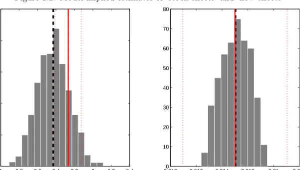
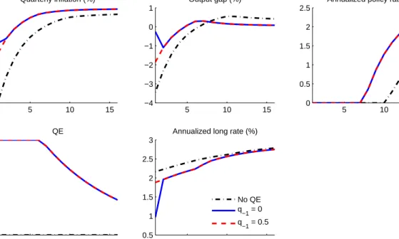
1.4 Modal simulation of a severe recessionary scenario . . . 51
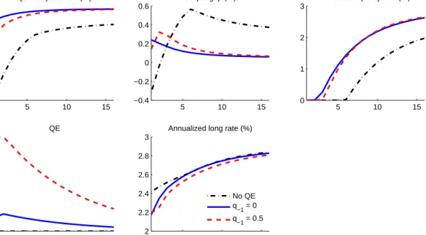
1.5 Modal simulation of a mild recessionary scenario . . . 52
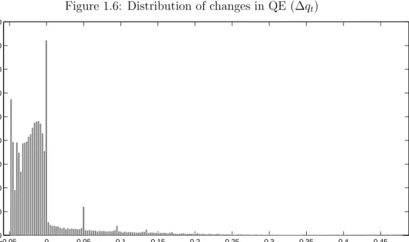
1.6 Distribution of changes in QE (∆qt) . . . 53
1.7 Mean outcomes under ‘permanent QE’ and alternative inflation targets . 58 1.8 Mean outcomes with active QE under alternative delegated loss functions 60 1.9 Distributions of portfolio revaluation K for alternative ¯q . . . 65
1.10 Distributions of variables at liftoff . . . 68
1.11 Policy functions for alternative parameter values . . . 70
1.12 Policy functions for alternative ¯q . . . 71
2.1 A government spending increase under debt financing and money financing117 2.2 Government spending increase financed via interest-bearing money vs debt119 2.3 Responses to a preference shock under alternative monetary policy rules 121 2.4 A money-financed transfer at the effective lower bound . . . 125
2.5 A permanent money-financed transfer at the effective lower bound . . . . 128
2.6 A money-financed transfer at the effective lower bound: cash in advance model . . . 131
2.7 Marginal effects of money-financed transfers in different model variants . 133 2.8 Money-financed transfers at the lower bound: additively separable money 135 2.9 Money-financed and debt-financed government spending with γ = 1 . . . 142
2.10 Financing government spending with interest-bearing money: additively separable case . . . 143
3.1 Solutions for Fˆπ and Fdˆ . . . 197
3.2 Responses to shocks: baseline model and New Keynesian benchmark . . 199
3.3 Responses to shocks under ‘average’ and ‘long’ debt duration . . . 201
3.4 Normalized losses for each model variant . . . 203
3.6 A recessionary scenario that causes the ZLB to bind . . . 208
3.7 An expansionary shock with for different assumptions about initial debt . 211 3.8 Recessionary scenario under average debt levels . . . 213
3.9 A debt reduction scenario . . . 216
3.10 The fiscal risk environment . . . 220
3.11 Debt reduction with fiscal risk: baseline model . . . 222
3.12 Debt reduction with fiscal risk: long duration debt variant . . . 224
3.13 Ex ante probabilities of fiscal rule switch . . . 228
3.14 Debt reduction with endogenous fiscal risk: baseline model, ξ= 46 . . . . 230
3.15 Endogenous probability function, (3.33), for ξ= 10 and ξ= 46 . . . 231
3.16 Debt reduction with endogenous fiscal risk: baseline model, ξ= 10 . . . . 232
3.17 Debt reduction with zero perceived fiscal risk: baseline model . . . 233
3.18 Ex ante probabilities of switch to active fiscal policy rule . . . 234
3.19 Expected losses when effects of endogenous probabilities are internalized and ignored . . . 235
3.20 Debt reduction experiment with deviation from time consistency . . . 236
3.21 Global analysis of Fπˆ and Fdˆ. . . 256
3.22 Responses to shocks in baseline model: time-consistent policy and com-mitment . . . 258
1.1 Parameter values . . . 37
1.2 Statistics from model simulations . . . 56
1.3 Model statistics for alternative parameterisations . . . 62
1.4 Model statistics for alternative ¯q. . . 72
2.1 Model parameters . . . 113
3.1 Baseline parameter values . . . 193
3.2 Macaulay duration of domestic government debt, selected countries . . . 193
3.3 Shock process parameters . . . 206
3.4 Summary statistics from alternative model variants . . . 210
The interaction of monetary and fiscal policy has been the subject of extensive study for many years. The wide range of important questions in this area has generated several strands of literature. For example, Blinder (1982) examines the appropriate level of coordination between monetary and fiscal policies using Tinbergen-Theil analysis, large scale macroeconomic models and game-theoretic approaches.
Indeed, analysis of these questions predates modern economics, in part because many central banks were formed to assist in the financing of the central government (for example, in France, Spain and the United Kingdom). For the United Kingdom, Ricardo (1824) discusses the incentives for the government to use monetary policy for fiscal purposes.
However, the recent experience with interest rates at the zero lower bound has raised new questions.
Shortly after the Global Financial Crisis in 2007–8, short-term policy rates in the United States and United Kingdom reached their lower bounds. Policymakers embarked on large scale purchases of assets (primarily government debt) financed by the creation of central bank reserves. This unconventional policy – commonly known as quantitative easing (QE) – was introduced in a bid to stimulate the economy, when conventional instruments were unavailable. Such policy measures were introduced without a clear understanding of some key questions. For example, how should QE be optimally used alongside the short-term policy rate? Is there scope for QE to become part of the conventional monetary policy toolkit?
Unconventional monetary policies were accompanied by discretionary fiscal stim-ulus in a number of countries. However, many of these programs were reversed, at least in part because of concerns about rapidly rising government debt. How should monetary policy be optimally conducted if the government is unwilling or unable
While the monetary and fiscal responses to the financial crisis were bold and unprecedented, some economists and commentators have proposed even more radical policy options. In particular, some have argued that financing government spending increases, tax cuts or direct monetary transfers to households by printing money would boost spending when in an economy trapped at the zero bound. Others argued that such policies risked creating runaway inflation. What are the possible effects of such ‘monetary financing’ policies in a standard macroeconomic framework?
This thesis addresses these questions.
Chapter 1 looks at the optimal use of quantitative easing (‘QE’): the purchase of long-term government bonds by the central bank, financed by the creation of reserves. It adds to the literature by studying the optimal deployment of QE in a model containing a ‘portfolio balance channel’. This is the mechanism through which most monetary policymakers believe that QE operates.
Portfolio rebalancing effects arise from the assumption that the relative demand for assets in an investor’s portfolio will depend on their relative returns. The mech-anism that captures this effect in the model follows the ideas of James Tobin and William Brainard in the 1950s and 1960s. Different assets are imperfect substitutes because they have individual non-pecuniary properties that investors value. In the model, investors face a particular type of portfolio adjustment costs that give rise to asset demand functions similar to those studied by Tobin and Brainard.
The presence of a portfolio balance effect creates the potential for a policymaker to influence relative asset prices by altering the relative supplies of assets available to investors. In particular, QE reduces the available supply of long-term government bonds, which increases their price and hence reduces long-term interest rates. A reduction in long-term interest rates can be used to stimulate spending and hence inflation when the short-term interest rate is stuck at its lower bound.
The model is calibrated to match evidence on the effects of QE in the United States. I use the model to study how QE should be optimally used alongside the
term government debt purchased by the central bank cannot be negative or exceed a pre-specified upper bound. This upper bound can be interpreted as a proxy for central bank solvency concerns highlighted by some monetary policymakers.
The analysis delivers three main results. First, QE is only adopted when the economy hits the zero bound and in such cases asset purchases are often large and occur rapidly. Second, exit from QE is gradual. Third, QE policy generally starts to tighten before the policy rate rises from the ELB.
The first two results are consistent with both observed QE policies and com-munications about exit plans by policymakers in the United Kingdom and United States. But the third result is not consistent with the observed behavior of both the FOMC and the MPC: ‘liftoff’ from the zero bound has preceded a QE unwind. I demonstrate that the third result could be reconciled with actual policy behavior by accounting for the fact that total total government debt was rising during the period of large scale asset purchases, a factor that is abstracted from in the simple model.
Chapter 2 studies fiscal policy actions financed by the creation of money. Vari-ants of this type of policy have been advocated in light of the slow recovery from the Global Financial Crisis in many economies, despite the deployment of unconven-tional policies, such as QE considered in Chapter 1. The use of monetary financing as a policy tool is regarded as even more unconventional or extreme than QE, given historical experiences of high inflation (or even hyperinflation) when governments have relied on money creation to finance their deficits.
I use a small sticky price model to examine the effects of two types of money-financed fiscal policies: using money creation to finance government spending and using money creation to finance direct transfers to households. The latter has some similarities to Milton Friedman’s famous ‘helicopter drop’ experiment.
With respect to money-financed government spending increases, I verify exist-ing results regardexist-ing their apparently powerful effects. Specifically, money-financed government spending has large effects on output and inflation because this policy
the inflationary effects of a government spending increase.
I contribute to the literature by extending existing results to demonstrate that the adoption of a money-financing rule may generate very poor macroeconomic outcomes in response to other economic shocks, such as an unanticipated change in private sector demand.
These results show that the effects of adopting a monetary financing rule stem from the implications of that rule for the behavior of the short-term nominal interest rate, rather than a special role for money.
The subsequent analysis focuses on money-financed transfers to households, re-lying on two model features. First, that money may earn a strictly positive rate of return. Second, a simple financial friction implies that households regard govern-ment liabilities as net wealth.
The fact that money earns interest allows control of the stock of money inde-pendently of the short-term bond rate. So monetary transfers can be used without altering the monetary policy response to shocks away from the zero bound. The financial friction creates a special role for money (and other government liabilit-ies). Importantly, it introduces an incentive to spend, rather than save, a monetary transfer from the government.
Simulations of money-financed transfers to households demonstrate that they can increase spending and inflation when the short-term nominal interest rate is temporarily stuck at the lower bound. Moreover, such transfers increase household wealth and hence spending and inflation, even if they are implemented in the form of atemporary increase in the stock of money.
However, the results also suggest three reasons to be cautious about the use of money-financed transfers to stimulate spending and inflation. First, the scale of the monetary transfers required to deliver a meaningful increase in aggregate demand and inflation is likely to be extremely large. Second, the frictions in the model suggest that equivalent effects could be achieved by an increase in conventional
nature of the frictions giving rise to a meaningful role for money and the policy rule used to set the short-term bond rate.
While Chapters 1 and 2 examine alternative monetary and fiscal policy options close to the zero bound, they share a common assumption about the broad con-figuration of monetary and fiscal policies. In particular, fiscal policy operates in a so-called ‘passive’ fashion: taxes and/or spending are adjusted to ensure that the real government debt stock is stabilized for any path of prices. This behavior means that the government’s intertemporal budget constraint is irrelevant for the monetary policymaker.
Chapter 3 studies the opposite case: fiscal policy is ‘active’ and monetary policy decisions must ensure that the real value of (nominal) government debt is stabilized. This policy configuration is sometimes called ‘fiscal dominance’.
I use a textbook New Keynesian model extended to include long-term nominal government debt. While the presence of this debt has no implications for optimal monetary policy under the textbook assumption of passive fiscal policy, it plays an important role when fiscal policy is active.
I first ignore the lower bound on the short-term interest rate and demonstrate three key results.
First, the duration of government debt plays a key role in determining the equi-librium behavior of output and inflation and underpins the extent of the so-called ‘debt stabilization bias’.
Second, the monetary policymaker cannot fully offset disturbances to the natural rate of interest under active fiscal policy, giving rise to costly fluctuations in output and inflation (that are fully offset when fiscal policy is passive).
Third, welfare losses generated by shocks that generate a trade-off between sta-bilizing the output gap and inflation may be smaller under active fiscal policy than passive fiscal policy. A cost-push shock that reduces inflation today increases the real value of outstanding nominal government debt. Stabilizing the real debt stock
These results also provide intuition for the behavior of the model in the presence of a lower bound on the short-term interest rate. My key result is that when the lower bound is accounted for, welfare losses may be smaller when fiscal policy is active than for the textbook model with passive fiscal policy.
This result is driven by the balance between two effects. Away from the zero bound, welfare losses are larger under active fiscal policy, since shocks to the natural rate of interest cannot be fully stabilized. But when the short-term interest rate is constrained by the lower bound, the combination of active fiscal policy and long-duration debt reduces welfare losses. Deflationary shocks that drive the policy rate to the lower bound raise the real value of government debt. This requires future policymakers to generate higher inflation to stabilize the debt stock, thus increasing inflation expectations. Higher inflation expectations at the lower bound reduce the real interest rate, stimulating spending and mitigating the recessionary effects of the deflationary shock. If the duration of government debt is long enough, the reduction in welfare losses at the zero bound outweighs the higher welfare losses from poorer performance away from the zero bound.
Finally, I consider the effects of a risk that fiscal policy behavior switches from passive to active during a debt reduction program. These experiments are motivated by recent debates over fiscal sustainability and so-called austerity programs in many countries. While the debt reduction program has no implications for the output gap or inflation under passive fiscal policy, even a small risk that fiscal policy becomes active can generate sizable effects. In the event that fiscal policy does become active in the future, delivering the debt reduction program will require higher inflation. The risk of higher future inflation increases expected longer-term inflation expectations and the optimal time consistent policy is to allow inflation to rise in the near term.
Optimal quantitative easing
Abstract
I study optimal monetary policy in a simple New Keynesian model with portfolio adjustment costs. Purchases of long-term debt by the central bank (quantitative easing; ‘QE’) alter the average portfolio return and hence influ-ence aggregate demand and inflation. The central bank chooses the short-term policy rate and QE to minimize a welfare-based loss function under discretion. Adoption of QE is rapid, with large scale asset purchases triggered when the policy rate hits the zero bound, consistent with observed policy responses to the Global Financial Crisis. Optimal exit is gradual. Despite the presence of portfolio adjustment costs, a policy of ‘permanent QE’ in which the central bank holds a constant stock of long-term bonds does not improve welfare.
1.1
Introduction
Central bank purchases of long-term government debt – often called quantitative easing (QE) – have been deployed as a monetary policy tool since the depth of the Great Recession, when short-term policy rates became constrained at their effective lower bounds. The widespread use of an unconventional monetary policy instru-ment has spawned much research. Perhaps surprisingly, however, there has been relatively little investigation of the optimal conduct of monetary policy when QE is a policy instrument, though recent contributions include Cui and Sterk (2018), Darracq Pari`es and K¨uhl (2016), Harrison (2012), Reis (2017) and Woodford (2016). In this chapter I study the optimal use of QE alongside the short-term policy rate
using a model that captures a ‘portfolio balance’ mechanism. This is the predomin-ant channel through which most monetary policymakers believe that QE affects the economy. I extend the textbook New Keynesian model (Gal´ı, 2008; Woodford, 2003) to include a bond market friction, following Andr´es, L´opez-Salido, and Nelson (2004) and Harrison (2012). The representative household faces portfolio adjustment costs when allocating its assets between short-term and long-term bonds.
Portfolio adjustment costs create a wedge between returns on short-term and long-term bonds that can be influenced by changes in the relative supplies of assets, thus providing a role for QE as a policy instrument. In addition to the direct (‘stock’) effects of asset purchases on relative bond yields, the adjustment cost specification also captures ‘flow effects’ of QE purchases (the effects on changes in the stocks of long-term and short-term bonds held by households). The adjustment costs are calibrated to match estimates of the stock and flow effects of QE on US long-term bond yields by D’Amico and King (2013).
The monetary policymaker acts under discretion to minimize a loss function de-rived from a quadratic approximation to the welfare of the representative household. In addition to the standard New Keynesian terms in inflation and the output gap, the loss function includes terms in the quantitative easing instrument. These arise because the portfolio adjustment costs through which QE has traction are welfare reducing.
The model is solved using projection methods, accounting for the non-linearities generated by the zero bound on the short-term interest rate and the possibility that bounds may also apply to the QE instrument (for example, the central bank’s holdings of long-term debt must be non-negative).
I study entry into and exit from a ‘QE regime’, defined as a period during which the central bank holds a positive stock of long-term bonds on its balance sheet. I find that entry into QE regimes can be rapid, with large scale asset purchases commencing as soon as the short-term policy rate hits the zero bound. Exit from QE is slower in order to mitigate the costs of changes in the portfolio mix.
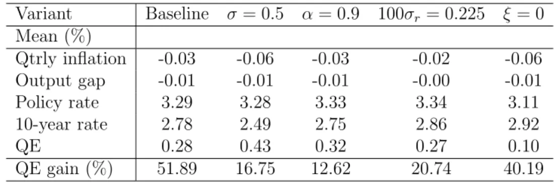
Relative to the case in which the only policy instrument is the short-term interest rate, use of QE reduces the welfare costs of fluctuations by around 50%. In this
‘active QE’ case, the central bank holds a positive stock of long-term bonds on average. On average, the long-term interest rate is below the short-term rate.
These observations suggest that a policy of ‘permanent QE’ in which the central bank is instructed to hold a constant stock of long-term bonds on its balance sheet may mitigate the effects of the zero bound on the short-term interest rate, by in-creasing the average short-term interest rate. However, I show that this is not the case.
While permanent QE does succeed in ‘twisting’ the term structure on average (the long-term rate falls and the short-term policy rate rises), this has little effect on average inflation expectations. Raising average inflation expectations requires agents to expect that the central bank will cushion the effects of future deflationary shocks by purchasing assets if those shocks are sufficiently large to force the short-term policy rate to the zero bound. A permanent QE policy does not have this property. The welfare gains of ‘active QE’ are therefore generated by an expectation effect.
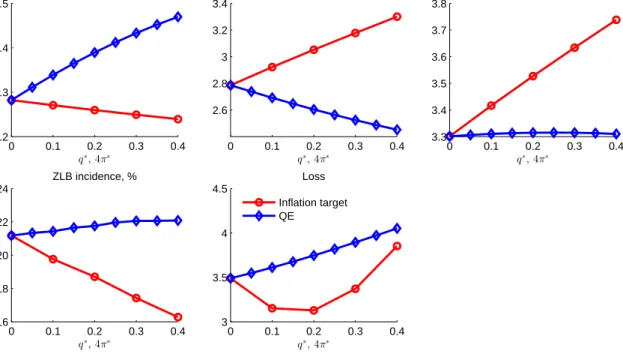
I also study the effects of delegation schemes by allowing the central bank to use both instruments, but instructing the central bank to minimize a loss function that differs from the one derived from household welfare. Consistent with similar analysis using textbook New Keynesian models, a small increase in the inflation target does improve welfare. However, increasing average inflation beyond a small amount generates welfare costs that outweigh the benefits associated with hitting the zero bound less frequently.
Allowing active use of QE but instructing the central bank to target a positive average quantity of long-term bonds on its balance sheet does not improve welfare relative to the case in which the central bank may freely choose the scale of QE. As in the case of permanent QE, this result stems from the fact that the most powerful effects of QE arise from the expectation that it will be deployed when necessary, rather than the direct effects of central bank asset holdings on long-term bond returns.
Several papers have studied QE using larger models featuring similar portfolio frictions: for example, Chen, C´urdia, and Ferrero (2012), Darracq Pari`es and K¨uhl (2016), De Graeve and Theodoridis (2016), Hohberger, Priftis, and Vogel (2017)
and Priftis and Vogel (2016). However, all of these papers assume that agents’ expectations satisfy a certainty equivalence assumption.1 With the exception of Darracq Pari`es and K¨uhl (2016) and Quint and Rabanal (2017), these papers do not consider the optimal design of QE policies. Neither Darracq Pari`es and K¨uhl (2016) nor Quint and Rabanal (2017) consider potential bounds on the QE instrument or use a welfare-based loss function.
The rest of this chapter is organized as follows. Section 1.2 discusses the ‘portfolio balance effect’ through which QE operates in the model and relates it to the broader literature on QE. Section 1.3 presents the model. Section 1.4 analyzes the optimal policy problem of a central bank tasked with using the short-term interest rate and QE to minimize a welfare-based loss function in a time-consistent manner. The results from the baseline parameterization of the model are presented in Section 1.5. Section 1.6 examines the effects of delegating alternative loss functions to the central bank. Section 1.7 assesses the robustness of the results to alternative assumptions about key parameter values and Section 1.8 concludes.
1.2
The portfolio balance mechanism
In an oft-quoted remark, former FOMC Chairman Ben Bernanke stated that “the trouble with QE is that it works in practice, but not in theory”.2 In this section, I argue that the so-called ‘portfolio balance’ mechanism has become the predominant channel through which most monetary policymakers believe that quantitative easing affects asset prices and the wider economy.
When quantitative easing was introduced as a response to the global financial crisis, there was uncertainty among policymakers about the channels through which the policy might operate and skepticism among academics that it would have any
1While the rational expectations assumption specifies that shocks are zero in expectation, the
certainty equivalence assumption specifies that these shocks are assumed (by agents) to be zero with certainty.
2The comment was made during a discussion session at the Brookings Institution: Bernanke
effect at all.3 For example, Benford, Berry, Nikolov, Young, and Robson (2009) doc-ument several possible channels through which quantitative easing might stimulate spending and inflation.4 Academic skepticism over the likely effects of the policy was typified by the analysis of Eggertsson and Woodford (2003), who demonstrated that a change in the composition of households’ portfolios would have no effect on equilibrium asset prices or allocations in a widely studied benchmark model.
A wide range of studies provided evidence that the quantitative easing policies enacted in response to the financial crisis increased asset prices and reduced longer-term interest rates.5 Other studies attempted to estimate the macroeconomic effects of these changes in asset prices and yields, with a general consensus that central bank asset purchases were successful in increasing output and inflation.6
Alongside the accumulating empirical evidence, economists explored possible the-oretical mechanisms that could give rise to such effects. From an asset pricing per-spective, King (2015) notes that the neutrality results of Eggertsson and Woodford (2003) rely on the (common) assumption of an additively time separable utility func-tion. This implies that the stochastic discount factor used to price assets depends only on consumption allocations across time. A broader class of utility functions imply that the stochastic discount factor also depends on the return on wealth (or the average portfolio return). In such cases, shifts in the composition of agents’ port-folios can affect the average portfolio return and hence individual rates of return via the stochastic discount factor.
King (2015) demonstrates that Epstein-Zinn-Weil preferences7 and the ‘preferred
3I focus on quantitative easing measures of the type introduced by several central banks in
response to the Global Financial Crisis. The Bank of Japan introduced a range of (somewhat different) balance sheet measures much earlier, given that it encountered the zero bound in the late 1990s.
4As well as the portfolio balance effect discussed in this section, the authors argue that the
expansion of bank reserves generated by asset purchases may create conditions that encourage bank lending and that asset purchases may help to anchor inflation expectations by signaling the central bank’s resolve to return inflation to target.
5Notable examples include D’Amico and King (2013), Greenwood and Vayanos (2010, 2014),
Joyce, Lasaosa, Stevens, and Tong (2011) and Krishnamurthy and Vissing-Jorgensen (2012).
6See, among many others, Baumeister and Benati (2013), Lenza, Pill, and Reichlin (2010),
Kapetanios, Mumtaz, Stevens, and Theodoridis (2012), Pesaran and Smith (2016) and Weale and Wieladek (2016).
habitat’ investor framework set out by Vayanos and Vila (2009) fit into the wider class of models in which portfolio composition affects asset prices.
The Vayanos and Vila (2009) model is an important contribution, as it provides a link with the strand of the macroeconomics literature, described below, to which this chapter contributes. The model features two types of agents, one of which has preferences for assets of a particular maturity which give rise to a downward sloping demand curve for the asset. The second type is an arbitrageur, trading in all assets. The interaction of the two agents gives rise to an equilibrium in which changes in the supply of an asset of a particular maturity affects the price of that asset (through the downward sloping demand of preferred habitat investors) and the prices of other assets with similar maturities (through the effect of arbitrage).
In macroeconomics, there is a long tradition of studying the effects of portfolio allocations on asset prices (and vice versa), dating back at least to the work of James Tobin and coauthors.8 The key assumption underpinning this theory is that the relative demand for alternative asset classes depend on their relative prices or returns, because of imperfect substitutability:
[A]ssets are assumed to be imperfect substitutes for each other in wealth-owners’ portfolios. That is, an increase in the rate of return on any one asset will lead to an increase in the fraction of wealth held in that asset, and to a decrease or at most no change in the fraction held in every other asset. (Tobin and Brainard, 1963)
These models assumed a (primitive) relationship between relative yields and rel-ative asset demands. Frankel (1985) showed that this type of asset demand could be derived as the solution to a Markowitz portfolio problem.9 As King (2015) notes, this approach does not incorporate rational expectations, because the portfolio problem does not account for the fact that future asset prices (which determine the rates of return on some assets) will be determined in the same way as current asset prices.
elasticity of intertemporal substitution is distinct from the coefficient of relative risk aversion. See Epstein and Zin (1989) and Weil (1990).
8See, for example, Tobin (1956, 1969) and Tobin and Brainard (1963).
9The investor’s objective function is the expected return on the portfolio, less a term in the
The seminal work of Andr´es et al. (2004) embedded portfolio adjustment costs into a New Keynesian rational expectations model to provide a more microfounded treatment of imperfect substitutability. The model echoes the finance approach of Vayanos and Vila (2009) and also features two types of agents.10 Unconstrained households have access to both short-term and long-term bonds, paying a port-folio adjustment cost when investing in the latter. Arbitrage by these households equates the returns (accounting for adjustment costs) of the two bonds. Constrained households only have access to long-term bonds. The consumption of constrained households is influenced by changes in the price of long-term bonds, which can be driven by changes in their relative supply via the portfolio adjustment costs paid by unconstrained households.
The Andr´es et al. (2004) model has been modified and extended in several direc-tions. Harrison (2012) builds a representative agent model in which all households face portfolio adjustment costs. In such a setting, aggregate demand depends on the average returns of short-term and long-term bonds as in Andr´es et al. (2004). However, there is no heterogeneity, so that the effect of long-term returns on ag-gregate demand depends on the (average) shares of long-term and short-term debt held by households rather than on the fraction of constrained households. This representative agent framework is arguably more tractable, in particular facilitating welfare analysis.11 Ellison and Tischbirek (2014) uses an indirect utility argument to directly impose portfolio balance terms in the asset pricing equations of the banks who manage portfolios on the behalf of households.12
Chen et al. (2012) develop a medium-scale model based on the Andr´es et al. (2004) setup, estimate it on US data and use it to study the effects of the FOMC’s
10Note, however, that the portfolio adjustment cost role for QE is somewhat different from the
role generated by the effects on portfolio risk studied in the finance context by, for example, King (2015).
11Welfare analysis is possible in models with heterogeneous agents, given an assumption about
how to measure social welfare. For example, Cui and Sterk (2018) study the welfare implications of QE in a state of the art heterogeneous agent New Keynesian (HANK) model by adopting a utilitarian definition of social welfare.
12In some ways, this approach has more similarities with the early models of Tobin and others,
though the indirect utility approach does deliver cross equation restrictions on the asset pricing relationships.
Large Scale Asset Purchase programs.13 Carlstrom, Fuerst, and Paustian (2017) adopt a market segmentation approach in which households invest in long-term government debt via leveraged financial intermediaries.
Once QE programs had been implemented and their effects observed, a consensus among monetary policymakers on the portfolio balance transmission channel seemed to emerge. For example, Bernanke (2010) argues that:
The channels through which the Fed’s purchases affect longer-term interest rates and financial conditions more generally have been subject to debate. I see the evidence as most favorable to the view that such purchases work primarily through the so-called portfolio balance chan-nel, which holds that once short-term interest rates have reached zero, the Federal Reserve’s purchases of longer-term securities affect financial conditions by changing the quantity and mix of financial assets held by the public.
Of course, while there may be near consensus among monetary policymakers on the transmission channel of QE, the portfolio balance effect is not without critique.14 Thornton (2014) challenges the empirical evidence on the effects of QE, finding little evidence of that QE operations had economically important effects on long-term bond yields.15
One alternative theory for the efficacy of QE is that it contains signals about the likely path for the short-term policy rate Bauer and Rudebusch (2014) provide some empirical evidence for this channel and Bhattarai, Eggertsson, and Gafarov
13Canzoneri and Diba (2005) and Canzoneri, Cumby, Diba, and L´opez-Salido (2008, 2011) have
explored models in which government bonds provide liquidity services so that the mix of assets held by private agents affects relative returns via liquidity premia. This complementary strand of the literature does not focus on the effects of quantitative easingper se.
14The discussion here focuses on quantitative easing operations in which the central bank
pur-chases long-term government debt (the focus of this chapter). In response to the financial crisis, some central banks also engaged in the purchase of private debt instruments. Such policies may be expected to operate through different channels and represent a complementary line of research. Important contributions include C´urdia and Woodford (2010), Del Negro, Eggertsson, Ferrero, and Kiyotaki (2017) and Gertler and Karadi (2011).
15These findings chime with the argument that Federal Reserve purchases of US government
debt constituted such a small fraction of total debt holdings that any portfolio balance effects would likely be very small (Bauer and Rudebusch, 2014; Cochrane, 2011).
(2015) provide a theoretical framework. Another theory is that changes in the composition of the central bank balance sheet can be used to reduce the risk exposure of private agents (Farmer and Zabczyk, 2016). Other authors have focused on the liabilities side of the central bank balance sheet, arguing that QE operates through the expansion of central bank reserves associated with asset purchases (see, for example, Aksoy and Basso, 2014; Reis, 2017).
The transmission mechanism in Cui and Sterk (2018) implies that both sides of the central bank balance sheet matter since QE involves a swap of relatively illiquid assets for more liquid assets (interpreted as reserves or bank deposits). Providing more liquid assets to households increases their ability to maintain consumption when they become unemployed, stimulating overall spending. This approach could be regarded as a microfounded variant of the ‘demand for liquidity’ narrative used by Andr´es et al. (2004) to motivate the type of portfolio friction used in their (and my) model.
My model can be seen as complementary to many of those discussed above, as QE may operate via several channels. However, my focus on a portfolio balance mechanism is prompted by the views of monetary policymakers cited above. So this chapter can be viewed as an exploration of what the portfolio balance mechanism implies for the optimal conduct of monetary policy.
1.3
The model
The model is a simple extension to the textbook New Keynesian model (Wood-ford, 2003; Gal´ı, 2008). This highlights the marginal implications of introducing an additional friction (portfolio adjustment costs) and hence the possible value of an additional monetary policy instrument, relative to a widely studied benchmark. Given the widespread use of the textbook model, in this section I focus on the additional features and relegate details of the derivation to Appendix 1.B.
1.3.1
Short-term and long-term bonds
There are two assets in the economy: short-term and long-term nominal govern-ment bonds. Following Woodford (2001), long-term governgovern-ment bonds are infinite maturity instruments, paying a geometrically declining coupon. Specifically, a bond issued at date t pays nominal coupons χs in dates t+ 1 +s, s≥ 0. This modeling
assumption is convenient because it implies that a one dollar holding of a bond issuedj periods ago is equivalent to aχj dollar holding of a bond issued today. The fact that the values of long-term bonds issued at different dates can be linked in this way means that it is possible to write budget constraints in terms of a single bond price and a single stock of long-term bonds.16
Consider first the nominal budget constraint of a representative household:
VtBeL,th +B h
t = (1 +χVt)BehL,t−1+Rt−1Bht−1+Wtnt+Tt+Dt−Ptct−Ψt (1.1)
The right hand side of the budget constraint captures income from working nt
hours at nominal wageWt, net transfers/taxesTtfrom the government and dividends
Dt from firms, less spending on consumption goods ct at price Pt and portfolio
adjustment costs Ψ (discussed in Section 1.3.2). The household decision problem will be analyzed in detail below: here I focus on the role of short-term and long-term bonds.
The household holds one-period bonds Bh, which pay a gross rate of return
R. The budget constraint with respect to short-term bonds is standard: bonds purchased at date t−1 mature in date t with a nominal payoff of Rt−1 per bond.
The household also holds long-term bonds, where BeLh denotes the number of bonds held, measured in terms of the equivalent quantity of newly issued bonds.
V is the nominal value (price) of each bond. The right hand side of the budget constraint contains the current value of existing holdings of the long-term bond. The quantity of long-term bonds purchased at all previous dates can be summarized in terms of a quantity of bonds (newly) issued in the previous period by virtue of the pricing relationship discussed above. The bond holdings from the previous period
e
BL,th −1 pay a coupon of 1 per bond in periodt and have valueχVt, reflecting the fact
that the quantityBeL,th −1 of datet−1 issued bonds has the same value as a quantity
χBeL,th −1 of date t issued bonds.
The budget constraint can be conveniently re-written in terms of the one-period return on long-term bonds:
BL,th +Bht =RL,t1 BL,th −1+Rt−1Bth−1+Wtnt+Tt+Dt−Ptct−Ψt (1.2) where: BL,th ≡VtBeL,th ; R 1 L,t ≡ 1 +χVt Vt−1
This formulation treats the choice variables of the household as thevalue of long-term bond holdings. Because households take bond prices as given this is isomorphic to the original formulation, but simplifies the model derivation. Similarly, the one period return is simply a definition expressed in terms of other asset prices. While the one-period return on long-term bonds is a sufficient statistic to characterize household behavior in the model, it is possible to map the implications for the one-period return back to bond yields that are more readily compared with the data, as shown below.
1.3.2
Households
The optimization problem of the representative household is
maxE0 ∞ X t=0 βtφt ( c1− 1 σ t −1 1− 1σ − n1+t ψ 1 +ψ )
wherecis consumption andnis hours worked. A preference shockφtis included and
will serve as the ‘demand shock’ that generates a persistent decline in the natural real interest rate considered in the simulation experiments examined below.
formulation of portfolio adjustment costs, Ψ:17 BL,th +Bht = RL,t1 BL,th −1+Rt−1Bth−1+Wtnt+Tt+Dt−Ptct − νP˜ t b h+bh L 2 " δ B h t Bh L,t −1 #2 − ξP˜ t b h+bh L 2 " Bth/BL,th Bh t−1/BhL,t−1 −1 #2 (1.3)
The portfolio adjustment costs have two components. The first component is a function of the deviation of the households ‘portfolio mix’, Bth
Bh L,t
from their desired level, δ−1. These adjustment costs are intended to capture ‘stock effects’: shifts in the supply of these assets can have a direct effect on their price. Following Andr´es et al. (2004),δis set equal to the steady-state ratio of long-term bonds to short-term bonds so that these portfolio costs are zero at the non-stochastic steady state.
The second component of the portfolio adjustment costs is a function of the
change in the household’s portfolio mix. This adjustment cost is motivated by the empirical evidence that changes in asset supplies associated with the auctions that implement asset purchases have an effect on the prices of assets purchased and their close substitutes (see D’Amico and King, 2013). In the context of my model, such ‘flow’ effects may be interpreted in terms of frictions in adjusting portfolios including transactions costs.
The tractability of this type of adjustment costs has led to their adoption in several monetary models.18 In reality, transactions costs are likely to be low, so the portfolio adjustment costs in the model are a stand in for a broader range of frictions. Andr´es et al. (2004) argue that they represent a perception by households that longer-term bonds are riskier than short-term bonds, such that households’ require a greater quantity of liquid assets (in their model, money) as compensation. Cast in this way, these costs may be better suited to inclusion in the utility func-tion. However, Harrison (2012) demonstrates that taking this approach gives rise
17Here bh andbh
L denote the steady statereal levels of short-term and long-term bonds. 18See, for example, Andr´es et al. (2004), Chen et al. (2012), De Graeve and Theodoridis (2016),
to isomorphic expressions for the model equations and welfare functions. Similarly, portfolio frictions in financial intermediation can give rise to very similar behavioral equations (Carlstrom et al., 2017; Harrison, 2011).
1.3.3
Firms
There is a set of monopolistically competitive producers indexed by j ∈(0,1) that produce differentiated products that form a Dixit-Stiglitz bundle that is purchased by households. Preferences over differentiated products are given by
yt = Z 1 0 y1−η −1 t j,t dj 1 1−η−t1
where yj is firm j’s output. The elasticity of demand among consumption varieties
ηt is assumed to be time-varying, which generates a ‘cost push’ shock in the Phillips
curve that characterizes log-linear pricing decisions.
Firms produce using a constant returns production function in the single input (labor):
yj,t =Anj,t
where A is a productivity parameter.
A fixed subsidy is assumed to ensure that the steady state is efficient. Calvo (1983) staggered pricing gives rise to a New Keynesian Phillips curve derived in Appendix 1.B.2 and discussed below.
1.3.4
Fiscal and monetary policies
To focus on the role of monetary policy, fiscal policy is highly simplified. There is no government spending and net transfers to households are lump sum. Of course, quantitative easing, by its nature, is a prime candidate for study from the perspective of monetary and fiscal policy interactions.19 My assumptions abstract from these considerations entirely.
19For example, Del Negro and Sims (2015) and Benigno and Nistico (2015) take such an approach
to examine the potential importance of the government and central bank intertemporal budget constraints.
Two aspects of these assumptions (detailed below) are intended to make quantit-ative easing an exclusively monetary policy operation. The assumption of a ‘neutral’ debt management policy (so that relative bond supplies are kept always in line with the desired holdings of households) gives the monetary policymaker maximal control over the debt stocks held by households. The assumption that the total value of debt is fixed implies that fiscal policy is ‘passive’ (in the sense of Leeper, 1991).20 As a result, the only non-neutrality from QE operates through the portfolio balance channel.21
To the extent that fiscal policy does not deliver the optimal mix of assets for households, the model would imply a role for QE in normal times (away from the zero bound). However, my assumptions are an attempt to capture the key elements of institutional arrangements in practice. For example, government treasury depart-ments (or their agents) are tasked with actively managing the maturity structure of government debt. Their mandate is typically expressed in terms of achieving favorable financing conditions for the government and ensuring adequate liquidity in government debt markets. In the context of my model, debt issuance in line with household portfolio preferences would (other things equal) minimize portfolio adjustment costs and hence the (social) costs of financing a given debt stock.
My assumptions also require that debt management policy remains unchanged when monetary policy uses QE at the zero bound. There is an active debate on the extent to which US government debt issuance may have offset some effects of FOMC asset purchases (see, for example, Greenwood, Hanson, Rudolph, and Summers, 2015). However, my assumptions are consistent with the institutional
20Tax revenues are adjusted to hold the debt stock constant which ensures that the government’s
intertemporal budget constraint is always satisfied, for any policy choices of the central bank. In particular, losses and gains on the central bank’s asset portfolios are immediately financed/rebated to private agents via lump sum taxes/transfers. As Benigno and Nistico (2015) point out, such a setup implies that only the consolidated government/central bank budget constraint matters for allocations.
21This focuses the analysis on the implications of the portfolio balance channel separately from
other mechanisms through which QE may operate. For example, Bhattarai et al. (2015) analyze the case in which the stock of long-term debt is a state variable in the model, because the government budget constraint is a constraint on policy actions. This setup gives rise to the possibility that QE can be used to provide a credible signal that interest rates will remain low in the future (the ‘signaling channel’). By assuming that government debt stocks are held fixed for all realizations of the short-term policy rate, this channel is eliminated from the model.
arrangements for QE in the United Kingdom, where the Debt Management Office was instructed to ensure that debt management operations “be consistent with the aims of monetary policy” including the asset purchases implemented by the Bank of England’s Monetary Policy Committee.22
Given the specification of the long-term bond discussed in Section 1.3.1, the nominal government budget constraint is:
Bt+VtBeL,t=Rt−1Bt−1+ (1 +χVt)BeL,t−1+Zt−Ptτt
where B and BeL represent stocks of short-term and long-term debt, Z denotes net
asset purchases by the central bank and τ represents net tax/transfer payments from/to households. The inclusion of Z reflects the assumption that QE is financed by the central government, as discussed below.
Applying the same change of variables introduced in Section 1.3.1 allows the constraint to be expressed in terms of the value of long-term bonds and their one-period return:
Bt+BL,t =Rt−1Bt−1+R1L,tBL,t−1+Zt−Ptτt (1.4)
The government implements the following debt issuance policies:
Bt Pt ≡ bt=b > 0, ∀t (1.5) BL,t Pt ≡ bL,t=δb, ∀t (1.6)
As discussed above, these issuance policies ensure that – absent QE operations by the central bank – households achieve their desired portfolio positions. Conditional on these issuance policies and QE by the central bank, net transfers to householdsT
are pinned down by the government budget constraint (1.4). In particular, changes in the value of the total government debt stock are transferred to/from households (lump sum) in order to keep the overall value of debt constant over time (a form of balanced budget financing).
22The quotation is from the letter from the Chancellor of the Exchequer to the Governor
of the Bank of England, 3 March 2009: http://www.bankofengland.co.uk/monetarypolicy/ Documents/pdf/chancellorletter050309.pdf.
Net purchases of long-term government bonds by the central bank are:23
Zt=VtQet−(1 +χVt)Qet−1
where the quantity of long-term bonds purchased by the central bank is denoted by
e
Q and it is assumed that coupon payments are paid to the central bank. Defining
Qt≡VtQet implies that:
Zt=Qt−R1L,tQt−1 (1.7)
The QE policy instrument is defined as the fraction of the market value of long-term bonds purchased by the central bank, denoted q:
Qt=qtBL,t
1.3.5
Market clearing and aggregate output
Market clearing for short-term and long-term bonds implies that:
bht =bt =b ;
Qt
Pt
+bhL,t =bL,t=bL
where lower case letters denote real-valued debt stocks (for example,bh
L,t ≡BL,th /Pt).
Combining the government debt issuance policy with the specification of the QE instrumentq gives:
bhL,t = (1−qt)δb
Goods market clearing implies that:
ct =yt− ˜ ν bh+bh L 2 " δ b h t bh L,t −1 #2 − ˜ ξ bh +bh L 2 " bh t bh t−1 bh L,t−1 bh L,t −1 #2
where total output satisfies:
yt = Ant Dt and Dt≡ R1 0 P jt Pt −η
dj is a measure of price dispersion across firms.
23In a model with money, the net expansion in the monetary base would also be included in this
expression. Here, QE is financed by a loan from the central government, which must ultimately be financed by lump sum taxes on households.
1.3.6
Model equations
As shown in Appendix 1.B, the log-linearized model can be reduced to an Euler equation for the output gap (ˆx) and a Phillips curve for inflation (ˆπ):24
ˆ xt=Etxˆt+1−σ h ˆ Rt−Etπˆt+1−γqt+ξqt−1 +βξEtqt+1−rt∗ i (1.8) ˆ πt=βEtπˆt+1+κxˆt+ut (1.9) where γ ≡ν+ξ(1 +β),ν ≡ν˜(1 +δ) and ξ ≡ξ˜(1 +δ). The ‘natural rate of interest’ isrt∗ ≡ −Et
ˆ
φt+1−φˆt
and the cost push shock is defined asut≡ −(1
−α)(1−βα)
α
η
η−1ηˆt. These variables follow exogenous processes given by: r∗t =ρrr∗t−1+ε r t (1.10) ut=ρuut−1 +εut (1.11) where εr t ∼N(0, σr2) andεut ∼N(0, σu2).
As shown in Appendix 1.D, the yield to maturity of the long-term bond is given by: ˆ Rt=χβEtRˆt+1 + (1−χβ) ˆ Rt−δ−1(1 +δ)γqt +ξδ−1(1 +δ)qt−1+βξδ−1(1 +δ)Etqt+1 ! (1.12)
1.3.7
Parameter values
Table 1.1 shows the baseline parameter values.25 It is convenient to scale the model by 100 to convert log-deviations into (approximate) percentage deviations.26 To do this, the standard deviations of the natural rate and cost-push shocks are scaled by 100. The portfolio adjustment cost coefficients, ν and ξ, are also scaled by 100, since the model equations are derived by linearizing (rather than log-linearizing) with respect toq.27
24Here, ˆzt
≡ ln (zt/z) denotes the log-deviation of variable zt from its non-stochastic steady state,z. The equations are linearized (rather than log-linearized) with respect toq.
25The productivity parameterAis chosen to normalize output to unity in the steady state. 26So that an output gap of x= 1 corresponds to a gap of one per cent.
27The approach to scaling effectively multiplies all model equations by 100 to convert log
Table 1.1: Parameter values
Description Value Description Value
σ Intertemporal substitution elasticity 1 χ Long-term bond coupon decay rate 0.975
κ Slope of Phillips curve 0.0516 δ Ratio of long-term to short-term bonds 0.3
β Discount factor 0.9918 b+bL Total debt stock (relative toquarterlyGDP) 2
ρr Autocorrelation, natural rate 0.85 100ν Adjustment cost (portfolio mix) 0.105
100σr Standard deviation, natural rate 0.25 100ξ Adjustment cost (change in portfolio mix) 3.2
ρu Autocorrelation, cost push shock 0
¯q Lower bound on QE 0
100σu Standard deviation, cost push shock 0.154 q¯ Upper bound on QE 0.5
η Elasticity of substitution 7.66
α Probability ofnot changing price 0.855 ψ Inverse labor supply elasticity 1
The key parameters of the aggregate demand and pricing equations areσ and κ. Settingσ = 1 is a standard assumption in the literature. Many studies that examine optimal policy at the zero bound use a much higher value (Adam and Billi, 2006; Bodenstein, Hebden, and Nunes, 2012; Levin, L´opez-Salido, Nelson, and Yun, 2010, among others, use a value of 6 or above). As Levin et al. (2010) point out, such calibrations are often required to generate significant effects on output at the zero bound under optimalcommitment policy in a canonical New Keynesian model. As I focus on the case of optimal discretionary policy, the zero bound has substantial effects even with a value for σ that is more in line with empirical evidence (such as that presented by Guvenen, 2006).
The slope of the Phillips curve (κ = 0.0516), though larger than the values used in similar studies (typically around 0.02–0.024), is consistent with my choice of a lower value for σ, given the values for the other parameters.28
The value of β is chosen to be consistent with a real interest rate of 3.35% in the non-stochastic steady state. As shown by Adam and Billi (2007), asβ increases, the steady-state real interest rate falls and so the chances of encountering the zero bound (and the costs associated with hitting it) increase.29
not require scaling in this way. To preserve the model relationships, the coefficients multiplyingq
are therefore multiplied by 100.
28Given the assumed elasticity of disutility of labor supply (ψ = 1), achieving this value of κ requires setting α = 0.855. This high degree of price stickiness is consistent with estimates from macroeconomic models such as Smets and Wouters (2005). More plausible estimates of average contract length can be obtained by adopting more flexible formulations of the demand for alternative product varieties as demonstrated by Smets and Wouters (2007). The value ofη= 7.66 is commonly used in the canonical New Keynesian model (see, for example, Adam and Billi, 2006; Bodenstein et al., 2012).
Other parameters that are important in determining the incidence of the zero bound are those governing the shock processes. The process for the natural real interest rate is assumed to be persistent, with ρr = 0.85, following Levin et al.
(2010). The standard deviation of the shock is roughly in line with the value used by Adam and Billi (2006) in their ‘RBC calibration’ and the values of the parameters governing the cost push shock are also taken from that calibration.
The parameters related to long-term and short-term bonds deserve particular attention. The value ofχis chosen to imply that the long-term bond has a duration of between 7 and 8 years in the non-stochastic steady state (see Appendix 1.D). This corresponds to the average duration of 10-year US Treasuries at the time of the first large scale asset purchase programme (D’Amico and King, 2013). I therefore interpret the long-term bond as a 10-year bond for the purposes comparing the model predictions with the data.
The steady-state ratio of government debt to (quarterly) GDP (i.e., b+bL)
is set to 2, in line with the findings of Reinhart, Reinhart, and Rogoff (2012). They estimate an average debt to (annual) GDP ratio of around 50% for advanced economies over the pre-crisis period. The steady-state ratio of long-term to short-term bonds (δ) is set to 0.3 on the basis of the data presented in D’Amico and King (2013).30
The values for the parameters governing the portfolio adjustment costs, ν and
ξ are designed to capture the empirical effects of quantitative easing, defined as ‘stock effects’ and ‘flow effects’ by D’Amico and King (2013). To arrive at these parameter values the model was solved on a grid of {ν, ξ} pairs and the values that
studies, including Adam and Billi (2007). Nevertheless, this value may be considered rather high, even by pre-crisis standards. The calibration is best thought of as an assumption about the non-stochastic steady-state nominal interest rate, because the efficient inflation rate in the model is zero.
30The ratio can be inferred from the data on the dollar amounts and percentages of stock
purchased displayed in D’Amico and King (2013, Fig 1) where short-term bonds are interpreted as those with an outstanding maturity of six years or less. Debt management strategies differ over time and across countries. Kuttner (2006, Figure 3) suggests that the average fraction of short-term (less than five-year maturity) bonds held by the private sector was around 25% over the period from 1965 to 2006, suggestingδ≈3. The data underlying Figure 1.1 suggestsδ >1 for the United Kingdom.
generated stock and flow effects closest to those estimated by D’Amico and King (2013) selected. This procedure and the results are discussed in Section 1.5.1.
Andr´es et al. (2004) estimate a parameter similar to ν (relating the long-term bond premium to household’s relative holdings of money and long bonds) using US data. Their estimate implies a value of 100×ν of around 0.035, though the long-term rate in that study is a three-year bond, a somewhat shorter maturity than the focus of my model. The evidence presented in Bernanke, Reinhart, and Sack (2004) would, using a simple back of the envelope calculation, suggest a much larger value for 100×ν ≈2.31 Of course, such calculations ignore the fact that asset purchases will have effects on other asset prices (in particular, expected short-term rates). The simulation approach discussed in Section 1.5.1 attempts to overcome these issues.
The finding that flow effects appear to be more important than stock effects (since ξ > ν) is consistent with the results of De Graeve and Theodoridis (2016). They estimate a flexible functional form for the mapping between maturity structure and the long-short bond spread and find that the data prefers a specification close to a first difference specification (implyingν ≈0 in the context of my model).
Finally, the parameters
¯q and ¯q represent the lower and upper bounds on the scale of QE operations that the central bank may undertake. Recall thatqrepresents the fraction of the total quantity of outstanding long-term bonds held by the central bank. Under the assumption that the central bank cannot issue long-term bonds that are perfect substitutes for long-term government bonds,qt≥0, and I set
¯q= 0. It must also be the case that ¯q ≤ 1, since the central bank cannot purchase more than 100% of the existing stock of long-term bonds. There may be practical reasons why the upper bound on asset purchases is less than 1, for example if there are some financial institutions that must hold long-term safe assets for regulatory
31This is calculated using a steady-state version of equation (1.12), assuming that an asset
purchase operation of size q = 0.1 is permanent and there are no effects on short-term rates long-term bond returns. To see this note that, since 100γ≡100ν+ 100ξ(1 +β), equation (1.12) can be written as ˆ Rt=χβEtRˆt+1+(1−χβ) ˆ Rt− 1 +δ−1100νqt −100ξ 1 +δ−1∆qt+β100ξ 1 +δ−1 Et∆qt+1 . A ‘steady state’ version of the equation sets ˆzt = ˆz,∀t so that ˆR = ˆR − 1 +δ−1100νq
and hence ∂Rˆ
∂q = − 1 +δ−
1100ν. Since ˆ
R is measured in quarterly units, we require 0.1× 1 +δ−1100ν= 0.25 which implies 100ν ≈2.