TENSOR DICTIONARY LEARNING WITH SPARSE TUCKER DECOMPOSITION
Syed Zubair and Wenwu Wang
Centre for Vision, Speech and Signal Processing
University of Surrey, Guildford, GU2 7XH, UK
Emails: [email protected], [email protected]
ABSTRACT
Dictionary learning algorithms are typically derived for deal-ing with one or two dimensional signals usdeal-ing vector-matrix operations. Little attention has been paid to the problem of dictionary learning over high dimensional tensor data. We propose a new algorithm for dictionary learning based on ten-sor factorization using a TUCKER model. In this algorithm, sparseness constraints are applied to the core tensor, of which the n-mode factors are learned from the input data in an al-ternate minimization manner using gradient descent. Simu-lations are provided to show the convergence and the recon-struction performance of the proposed algorithm. We also apply our algorithm to the speaker identification problem and compare the discriminative ability of the dictionaries learned with those of TUCKER and K-SVD algorithms. The results show that the classification performance of the dictionaries learned by our proposed algorithm is considerably better as compared to the two state of the art algorithms.
Index Terms— Tensor Factorization, Sparse Representa-tions, Classification, Dictionary Learning
1. INTRODUCTION
Learning the features and structures of a signal is important for obtaining a succinct representation that can be used for various applications such as source separation and signal classification. Dictionary learning algorithms emerging from sparse representations have recently been used for learning such representations as given in [1]. However, these algo-rithms are mostly limited to one or two dimensional signals. With content-rich applications emerging nowadays, signal dimensionality is constantly increasing e.g. in video sig-nals. Moreover, a low-dimensional signal such as an audio signal can be cast in a higher dimensional space, e.g. in a space-time-frequency domain. This preserves the structure of the signal which may otherwise be lost when used in a low dimensional form. Hence, it becomes highly desirable for those algorithms to be able to learn signal features from higher dimensional data, such as tensor data.
Tensor factorization and decomposition have recently attracted attention in the signal processing community, for processing high dimensional signals. PARAFAC [2] and TUCKER [3] decompositions are two such classical algo-rithms. PARAFAC decomposes the tensor as a sum of k rank-1 tensors while the TUCKER method computes the or-thonormal subspaces corresponding to each mode of the ten-sor. This can be treated as higher order principal component analysis. However, these methods do not explicitly enforce signal sparsity despite its benefits in signal representations for various applications.
Recent effort has therefore been on extending these two algorithms by introducing additional constraints to the models with the aim of learning sparse representations of the tensors. Both non-negativity and sparsity have been used to achieve this. Inspired by the non-negative matrix factorization (NMF) techniques due to Lee and Seung [4], the authors of [5] and [6] introduced non-negative PARAFAC decomposition with multiplicative updates and applied it to various signal and im-age processing applications. Similarly, non-negative versions of TUCKER decomposition have also been proposed in [7] and [8].
Sparse representations of PARAFAC and TUCKER mod-els have also been derived. In the case of TUCKER model, which is the focus of our discussion in this paper, sparse TUCKER decomposition methods have been proposed in [7] and [9]. In [7], smoothing matrices are used for each mode of the tensor to make the core tensor as well as the TUCKER factors sparse, while in [9], sparsity is introduced by penal-izing its core tensor withl1norm and claim that this penalty
can also be applied to any of the other factors of TUCKER decomposition. In both of these works, sparsity has been applied in case of non-negative TUCKER decomposition. Hence the factors of TUCKER decomposition are learned by NMF techniques with multiplicative updates as presented in [4].
In this paper, we propose a tensor dictionary learning algorithm based on the TUCKER model with sparsity con-straints over its core tensor. Unlike [7] and [9], the sparsity over the core tensor is applied here in a greedy fashion. The sparse core tensor is calculated by a tensor extended version of the greedy algorithm, Tensor Orthogonal Matching Pursuit
(TOMP) [10]. Two main reasons for introducing sparsity in the core tensor are as follows:
• Unlike the standard TUCKER representation, the spar-sity of the core tensor compresses the data by consider-ing only non-zero values of the core tensor. Moreover, the input signal is represented by only those columns of mode-n dictionaries which correspond to those non-zero elements of the core tensor.
• The core tensor establishes the relationship between the elements of the dictionaries for describing the in-put data model. Non-sparse core tensor makes this relationship ambiguous specially in decision based ap-plications such as classification. The sparsity of the core tensor reduces this ambiguity and clarifies the relationship between the dictionaries.
To learn tensor dictionaries of TUCKER model along each mode, we propose a gradient descent algorithm that updates the mode-n dictionaries iteratively in an alternating manner. The proposed tensor dictionary algorithm, similar to standard dictionary learning algorithms, is a two-stage iterative pro-cess: sparse coding and dictionary update. First, given initial TUCKER factors considered as dictionaries, the TOMP al-gorithm is used to find the sparse core tensor. Then in the second stage, the dictionaries (factors) corresponding to each mode are updated, using the gradient descent method.
The organization of the whole paper is as follows: Section 2 formulates an objective function for tensor dictionary learn-ing problem. Section 3 presents the Tensor OMP algorithm. Section 4 describes the proposed dictionary learning method for high dimensional data, GradTensor. Section 5 shows ex-periments along with their results and section 6 concludes the paper.
2. PROBLEM FORMULATION AND OPTIMIZATION CRITERION
A signal of a high dimension is considered as a tensor. Here for simplicity, we consider Y as a tensor of three dimensions e.g. Y ∈ RI1×I2×I3, whereI
n(n = 1,2,3)are the
dimen-sions of each mode. However, the following discussion can be readily extended to the signals with a dimension greater than three. A three dimensional tensor is also called as a three-way signal. A matrix is a form of two-way signal and a vector is considered as a one-way signal. A tensor can be unfolded to a mode-n matrix form and represented as Y(n). For a
three-way tensor, the mode-n matrix can be extracted by changing all the indices in the tensor except then-th index. Hence a three-way tensor can be unfolded into any of its mode-n ma-trices. For example, the mode-1 unfolded matrix of tensor Y, i.e. Y(1), has a dimension RI1×I2I3. Similarly the mode-2
unfolded matrix Y(2) has a dimensionRI2×I1I3. Tensor
de-composition for the TUCKER model is formulated as:
Y = X×1A×2B×3C (1) = M1 X m1=1 M2 X m2=1 M3 X m3=1 xm1m2m3am1◦bm2◦cm3
where ◦ is the outer product between the vectors. A ∈ RI1×M1, B ∈ RI2×M2 and C ∈ RI3×M3 are orthogonal
factor matrices composed of a, b and c vectors and can be considered as principal components along each mode of the tensor. X ∈ RM1×M2×M3 is a core tensor. This form
of decomposition was suggested by [3], hence it is called TUCKER decomposition. It can be represented element-wise as yi1i2i3 = M1 X m1=1 M2 X m2=1 M3 X m3=1 xm1m2m3ai1m1bi2m2ci3m3 (2) f or in= 1, . . . , In, n= (1,2,3)
If the core tensor X is super-diagonal andM1 =M2=M3,
then this can be considered as PARAFAC decomposition in-troduced by [2].
To learn tensor dictionaries with a sparsity constraint on the core tensor X , our objective function for model (1) takes the form: F(X,A,B,C) = min X,A,B,CkY−X×1A×2B×3Ck 2 F s.t. xm1m2m3 = 0∀(m1, m2, m3)∈ M/ 1× M2× M3 (3)
wherek · kF is the Frobenius norm,Mn = [m1n, . . . , msnn]
denotes the subset of indices of non-zero values in the core tensor for mode n (n= 1,2,3), andsnrepresents the
mode-n sparsity, showimode-ng the mode-number of selected colummode-ns of each dictionary required for the TUCKER representation. In this way, the sparsity structure of the core tensor isblock-sparse
and the total sparsity (i.e. the number of non-zeros) of the three way core tensor is denoted bys=s1×s2×s3. Here
we assume that the size of the core tensor X is larger than or equal to the size of Y (Mn≥In).
3. TENSOR OMP
Tensor OMP (TOMP) [10] is based on the equivalence of equation (1) to the vectorized version of the tensor represen-tation in terms of Kronecker dictionaries, i.e.
vec(Y) = (C⊗B⊗A)vec(X) (4) y = (C⊗B⊗A)x (5) where ⊗ is the Kronecker product. vec(·) is obtained by stacking all the columns of mode-1 tensor Y(1) in a single
vectory ∈ RI1I2I3. Equation (5) is similar to the
xis a sparse vector withsnumber of non-zero elements. This is one of the reasons for assumingMn ≥Inbecause sparse
signal model is formulated with an overcomplete dictionary. The TOMP algorithm is given in Algorithm 1.
Algorithm 1: Tensor-OMP
Require:Dictionaries A∈RI1×M1, B∈RI2×M2and C
∈RI3×M3, input signal Y, maximum number of non-zeros
coefficientstmax≤s, tolerance.
Output:X(M1,M2,M3) =E,{M1,M2,M3}.
Ensure:Sparse representation Y=X×1A×2B×3C with
xm1m2m3= 0∀(m1, m2, m3)∈ M/ 1× M2× M3.
(X(M1,M2,M3)) =E.
1. Mn= [∅](n= 1,2,3),R=Y,X=0, t= 1;
2. while|M1||M2||M3|< tmaxand||R||F > do
3. [mt1mt2mt3] =arg max[m1m2m3]|R×1A T (: , m1)×2BT(:, m2)×3CT(:, m3)|; 4. Mn=Mn∪[[mtn](n= 1,2,3),D1=A(: ,M1),D2=B(:,M2),D3=C(:,M3);
5. e=arg minu||(D3⊗D2⊗D1)u−y||22;
6. R=Y−E×1D1×2D2×3D3;
7. t=t+ 1; 8. end while
9. return{M1,M2,M3},E;
4. PROPOSED METHOD: GRADTENSOR The tensor dictionaries and the core tensor are computed in a two-step process. In the first step, the sparse core tensor is computed using TOMP with tensor dictionaries initialized byMn left leading singular vectors of the mode-n matrices
of input tensor Y . Once the sparse core tensor is obtained, the tensor dictionaries are computed iteratively by gradient descent in an alternating manner.
Mathematically, equation (1) can be represented in an un-folded form as
Y(1) = AX(1)(C⊗B)T
Y(2) = BX(2)(C⊗A)T (6)
Y(3) = CX(3)(B⊗A)T
To calculate mode-1 dictionary A in the unfolded form, the minimization of equation (3) can be written as
min
A kY(1)−AX(1)(C⊗B)
T k2
F (7)
From (7), the gradient of the error norm with respect to A can be calculated by ∇FA= (Y(1)−AX(1)(C⊗B)) X(1)(C⊗B)T † (8) where†is the pseudo-inverse of the matrix. Similarly, the gradients of the objective function with respect to B and C can be calculated as ∇FB= (Y(2)−BX(2)(C⊗A)) X(2)(C⊗A) † (9) ∇FC= (Y(3)−CX(3)(B⊗A)) X(3)(B⊗A) †
These gradients are then used to update the tensor dictionar-ies. The updates are given by
A(k+1)=A(k)−γ∇FA
B(k+1)=B(k)−γ∇FB (10) C(k+1)=C(k)−γ∇FC
whereγis the step size andkis the current step of the gradi-ent descgradi-ent algorithm. These tensor dictionaries are learned in an alternate minimization manner such that when learn-ing one dictionary like A, all the other dictionaries and the core tensor are held fixed. In this way, all the dictionaries are updated. In the next iteration, these learned dictionaries are used to find out the sparse core tensor in the sparse coding stage. This two-stage learning process alternates between ten-sor dictionaries learning and sparse core tenten-sor update until a stopping criterion is reached. Algorithm 1 gives the summary of the whole algorithm.
As these dictionaries are learned by the gradient descent, the minimization of the objective function may lead to local minima. To improve convergence, all the dictionaries are ini-tialized by the left leading factors of the input tensor data. Though we don’t have an explicit proof for the convergence of the algorithm, yet the simulations on synthetic data show the good convergence of the algorithm as confirmed in the next section.
Algorithm 2: GradTensor
Task:Find mode-n dictionaries A∈RI1×M1, B∈RI2×M2
and C∈RI3×M3and sparse core tensor X∈RM1×M2×M3
that give sparsest representation of input signal tensor Y∈RI1×I2×I3 with predefined sparsitys=s
1×s2×s3.
Require:Input signal Y, sparse core tensor X, maximum sparsity value (total number of non-zeros)s, step sizeγ, tolerance1and2,
Output:A,B,C.
Initialization:Mode-n dictionaries A, B and C each initialized byMnleft leading vectors of Yn, where
n= 1,2,3is the index of the modes of a tensor. Repeat until convergence:( i.e.F ≤2)
1. Sparse Coding Stage: Use TOMP to find sparse core
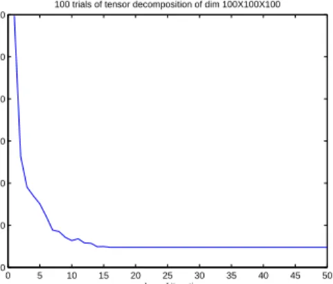
0 5 10 15 20 25 30 35 40 45 50 0 100 200 300 400 500 600 number of iterations Residual Error
100 trials of tensor decomposition of dim 100X100X100
Fig. 1. Convergence of GradTensor over 100 trials.
2. Dictionary Learning Stage: Learn dictionaries A, B, C
for each mode by the gradient descent.
• Calculate gradient for A,∇FA. While fixing all
the other dictionaries and sparse core tensor, update A by (8) and (10) for A until the error between two consecutive iterations reaches below or equal to1.
• Calculate gradient for B,∇FB. While fixing all
the other dictionaries and sparse core tensor, update B by using (9) and (10) for B until the error between two consecutive iterations reaches below or equal to1.
• Calculate gradient for C,∇FC. While fixing all
the other dictionaries and sparse core tensor, update C by using (9) and (10) for C until the error between two consecutive iterations reaches below or equal to1.
5. EXPERIMENTS AND RESULTS
We perform three different experiments to analyse our algo-rithm for different applications. Synthetic data is used to ex-amine the convergence of the algorithm. The second experi-ment includes image reconstruction by the learned tensor dic-tionaries with the sparse core tensor and the third experiment provides the classification performance of the algorithm for speaker identification in comparison with the TUCKER and the K-SVD [1] algorithms.
5.1. Simulation based on Synthetic Data
In the first experiment, we test the convergence of our pro-posed method by applying it on a synthetically generated ten-sor of sizeI1×I2×I3= 100×100×100. The tensor is
gen-erated from the mode dictionaries of size100×100and the sparse core tensor of sizeMn = 1.5In(n= 1,2,3)whose
el-ements are obtained from Gaussian distributions. The sparse
core tensor has a fixed mode sparsity ofµ=sn/Mn = 1/6.
The value of the step size γ is 0.3. There are two thresh-old parameters for stopping the algorithm,1for the gradient
descent and2for the whole algorithm. In the dictionary
up-date stage, when the error between two consecutive iterations reaches below or equal to1, dictionary update stops. In a
similar way, the whole algorithm stops when the error tween the input tensor and the reconstructed one reaches be-low or equal to2. Typically,1and2are chosen as10−6and 10−4 respectively. The algorithm convergence curve shown
in Figure 1 is obtained by averaging the curve over 100 inde-pendent trials (experiments).
5.2. Image Reconstruction Original image (a) Reconstructed image 1 (b) Reconstructed image 2 (c) Fig. 2. Comparison between the original image and the recon-structed images using two different sparsity levels of the core tensor. (a) The original Image. (b) The reconstructed image with the core tensor sparsity of 31%. (c) The reconstructed image with the core tensor sparsity of 12%.
For the second experiment, we learn high dimensional signal features for a 3-D human abdomen image of sizeI1×
I2×I3151×125×141by our proposed algorithm. This
dataset is given by [11]. Since we are interested in investigat-ing the effect of the core tensor sparsity on the signal recon-struction, not its dimensions with respect to the input tensor, hence we set Mn = 1.5In and the fixed mode sparsity as
µ= 1/2.2andµ= 1/3respectively, which is equal to 31% and 12% of the total sparsity level (number of non-zeros) of the core tensor, respectively. These sparsity levels compactly represent the input data even though Mn > In. The 50th
slice of the image is reconstructed by the learned dictionaries and the sparse core tensor, as shown in Figure 2, where the original image slice can be compared with the reconstructed slices using the two different levels of sparsity. It can be ob-served that the reconstructed image using the atoms learned by the proposed sparse tensor learning algorithm resembles the original image very nicely.
5.3. Speaker Identification
To compare the discriminative power of our proposed algo-rithm, we apply it for the multi-class classification problem
of speaker identification and compare its classification per-formance with that of the TUCKER algorithm [3] and K-SVD algorithm [1]. The signal classification is performed by pro-jecting feature matrix of test signals on to the basis learned by the learning algorithms. The basis in each case of GradTensor as well as the TUCKER algorithm is computed by
D=X×1A×2B (11)
whereDis the learned basis tensor. This basis tensorDis used to classify the test feature matrix and is determined dur-ing the traindur-ing phase. By followdur-ing the equation (6), the input signal Y can be represented in terms of learned basis tensor in an unfolded form as
Y(1)=IAD(1)(C⊗IB)T (12)
whereIA andIB are the identity matrices of the same size
as A and B. For a 5-class speaker identification problem, the test feature matrixYtest is projected on to each class basis
tensor learned in the training phase. The class label of the basis tensor that gives the minimum residual error is the label of the test signal.
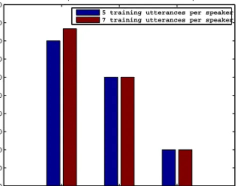
For this classification problem, a subset of the TIMIT cor-pus is selected for speaker identification of 5 speakers with 10 utterances (sentences) per speaker, resulting in a total of 50 utterances. For different numbers of utterances per speaker, we perform classification in such a way that the training and testing examples do not overlap with each other. The class specific basis which acts as the classifier, is learned in the training phase on Linear Predictive Coding (LPC) features of the training signals. The classification performance of the basis learned by three different algorithms (GradTensor, TUCKER and K-SVD) is shown in Figure 3. In case of ten-sors,Mn =Inand the fixed mode sparsity in GradTensor is
µ=sn/Mn = 1/10. In the case of K-SVD which learns the
dictionary from two dimensional training features, the size of the input training signal, dictionary size and sparsity level are same as those of GradTensor.
This classification example clearly shows the discrimi-native power of the class basis learned by the GradTensor over those learned by the TUCKER and the K-SVD. This also signifies the importance of learning a sparse core ten-sor. Since the core tensor in TUCKER decomposition estab-lishes the relationship between decomposition factors along each mode, sparsity constraint on the core tensor applied in the GradTensor learning algorithm clarifies this relationship and reduces the ambiguity in the interpretation of this rela-tionship. The classification results show that the sparsity con-straint also helps to maintain the discriminative ability of the learned dictionaries.
6. CONCLUSION
We have designed a tensor dictionary learning algorithm for the TUCKER model that incorporates sparsity constraints on
GradTensor TUCKER K−SVD 0 10 20 30 40 50 60 70 80 90 100 % classification accuracy
Classification performance for identification of 5 speakers
5 training utterances per speaker 7 training utterances per speaker
Fig. 3. Classification performances for the identification of 5 speakers for different decomposition algorithms with differ-ent number of utterances per speaker.
the core tensor. We show the convergence property of the pro-posed algorithm along with experiments on signal reconstruc-tion and classificareconstruc-tion. The reconstrucreconstruc-tion and classificareconstruc-tion results clearly show the ability of our algorithms for maintain-ing the discernmaintain-ing features of the signals while retainmaintain-ing the signal reconstruction. In future, we will explore the possibil-ities for further improving its discriminative ability by incor-porating additional constraints to the cost function, such as inter-class correlations, in order to learn class discriminative dictionaries.
7. REFERENCES
[1] M. Aharon, M. Elad, and A. Bruckstein, “K-SVD: An algorithm for designing overcomplete dictionaries for sparse representation,” IEEE Transactions on Signal
Processing, vol. 54, no. 11, pp. 4311–4322, 2006.
[2] R. A. Harshman, “Foundations of the parafac proce-dure: Models and conditions for an “explanatory” multi-modal factor analysis.,” UCLA working papers in
pho-netics, vol. 16, pp. 1–84, 1970.
[3] L. R. Tucker, “Some mathematical notes on 3-mode factor analysis.,” Psychometrika, vol. 31, pp. 279–311, 1966.
[4] D. D. Lee and H. S. Seung, “Algorithms for non-negative matrix factorization,” in Proc. Neural
Infor-mation Processing Systems, 2001, pp. 556–562.
[5] T. Hazan, S. Polak, and A. Shashua, “Sparse image cod-ing uscod-ing a 3d non-negative tensor factorization,” in
Proc. of IEEE International Conference on Computer
Vision, October 2005, vol. 1, pp. 50 – 57.
[6] E. Benetos and C. Kotropoulos, “Non-negative ten-sor factorization applied to music genre classification,”
IEEE Transactions on Audio, Speech and Signal
Pro-cessing, vol. 18, no. 8, pp. 1955–1967, November 2010.
[7] Y-D. Kim and S. Choi, “Nonnegative tucker decompo-sition,” inProc. IEEE Conference on Computer Vision
and Pattern Recognition., june 2007, pp. 1 –8.
[8] Y-D. Kim, A. Cichocki, and S. Choi, “Nonnegative tucker decomposition with alpha-divergence,” inProc. IEEE International Conference on Acoustics, Speech
and Signal Processing., 2008, pp. 1829 –1832.
[9] M. Mørup, L. K. Hansen, and S. M. Arnfred, “Algo-rithms for sparse nonnegative tucker decompositions,”
Neural Computing, vol. 20, no. 8, pp. 2112–2131, 2008.
[10] C. F. Caiafa and A. Cichocki, “Block sparse represen-tation of tensors using kronecker bases.,” inProc. IEEE International Conference on Acoustics, Speech and
Sig-nal Processing, 2012, pp. 2709–2712.
[11] J. Vandemeulebroucke, D. Sarrut, and P. Clarysse, “The popi-model, a point-validated pixel-based breathing tho-rax model,” in Proc. of the XVth ICCR Conference, 2007.