Architecture Blueprint for a Business Process
Simulation Engine
Stefan Krumnow1, Matthias Weidlich1, R¨udiger Molle2
1Hasso Plattner Institute, University of Potsdam, Germany 2ITAB, Hamburg, Germany
[email protected] [email protected]
Abstract:Simulation of business process models allows for drawing conclusions on the performance and costs of business processes before they are implemented or changed. Requirements for a business process simulation engine are specific to a concrete use case and a dedicated business domain. In this paper, we focus on the simulation of clinical pathways in a hospital. We elaborate on the requirements imposed by this use case in detail and propose an architecture blueprint for a simulation engine. It is based on annotated BPMN process models and uses timed and colored Petri nets as the underlying formalism.
Keywords: BPMN Process Models, Clinical Pathways, Discrete Event Simulation
1
Introduction
Business process modeling has proven to offer a successful way for capturing and specifying processes that are run in order to achieve a certain business goal. Process models support the understanding of existing processes as well as discussions on them. Moreover, they can be analyzed in order to find weaknesses and unintended behavior.
Models of intended processes cannot only be used to communicate new procedures but also for simulations of the new processes’ behaviors. Thereby, the creation and investigation of these models allows for early (and therefore particularly valuable) conclusions on the planned processes performance and costs. The same method is used in many engineering disciplines, such as the construction of a new car. Here, before the actual car is built, several prototypes capturing only the car’s shape are developed and tested in a wind tunnel. This paper proposes an architecture blueprint for a business process simulation engine. We focus on the use case of predicting the performance of clinical pathways that are defined by BPMN models. These models are supposed to capture relevant execution aspects, whereas their primary focus is still on human-to-human communication. Therefore, the simulator has to be integrated with BPMN modeling concepts seamlessly. Hence, our contribution is
an architecture proposal for a discrete event simulation of annotated BPMN models. To this end, we leverage timed and colored Petri nets.
The remainder of this paper is structured as follows. Section 2 presents our use case and derives requirements from it. Then, Section 3 examines existing performance prediction approaches. Based on these approaches, Section 4 proposes an architecture of a simulation engine supporting the introduced use case. Finally, Section 5 concludes the paper.
2
Clinical Pathway Simulation Use Case
This section introduces the background of our work. First, Section 2.1 elaborates on our use case. Second, we derive concrete requirements from the use case in Section 2.2.
2.1 Use Case
In this paper, we focus on the use case of simulation of clinical pathways. A clinical pathway describes the different steps during the interdisciplinary diagnosis and clinical treatment of a group of patients suffering from the same illness. Using process modeling languages such as the BPMN [omg09], clinical pathways can be captured in process models, e.g. for the purpose of standardization and clinical quality management.
However, there are also other possible applications for clinical pathway models: Transfer-ring process models from the current structure of an existing state (”as-is”) to the intended structure of the pathway after a change (”to-be”) can be used to reason over the impact the change will have, e.g. on patient waiting times, staff workloads, or total treatment costs. For a simulation, a process analyst creates a set of ”as-is” process models, which in this use case are BPMN 2.0 process diagrams. The models are to be quantified, i.e. measured or best educated guesses of activity efforts, cost and gateway probabilities are assigned. Also, additional simulation parameters such as the frequency of patients arriving or number of available nurses on a station are specified. Then, simulation is started and execution statistics are derived. The output should describe the real as-is situation for the selected group of patients. The procedure can then easily be repeated after some models or part of them had been changed to a proposed or planned ”to-be” situation. Within the statistics mentioned, we can now find answers to simulation questions such as the change of average waiting time of patients in the emergency room or changed resource utilisation.
Simulating a Business Process.As already mentioned, a clinical pathway describes how a
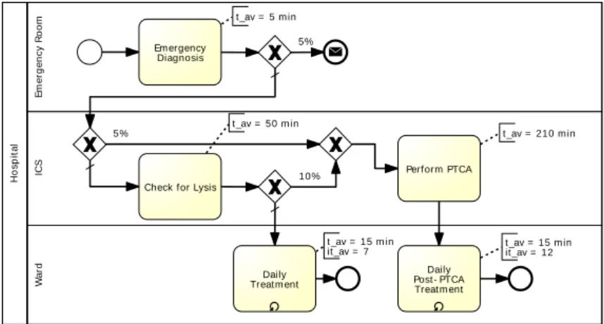
diagnosed patient is given therapy. Therefore, a process model of a clinical pathway consists of set of tasks and subprocesses as well as decision points and parallel executions. Pools and lanes can be used to assign roles and responsibilities to the actions that need to be performed in the course of the patient’s treatment. As many of these actions have to be conducted repeatedly, e.g. in nursing, loops are often used as well. Figure 1 shows an example of a clinical pathway model describing heart attack treatment. Due to space limitations, the
Heart Attack Treatment H o s p it a l E m e rg e n c y R o o m Em ergency Diagnosis t _av = 5 m in W a rd Daily Post - PTCA Treat m ent Daily Treat m ent t _av = 15 m in it _av = 12 t _av = 15 m in it _av = 7 IC S
Check for Lysis
Perform PTCA t _av = 210 m in t _av = 50 m in 5% 5% 10% Stefan Krumnow 1 of 1 23.06.2010
Figure 1: Abstract simplified clinical pathway treating a heart attack (modeled using BPMN)
model is simplified with respect to the number of activities and the distinction between different roles of hospital staff.
For a simulation of this model, not only the ordering of activities but also some execu-tion informaexecu-tion is relevant. Therefore, the process model is annotated with three basic performance values: a) Each task holds an averageduration. b) For each decision point, probabilitiesfor the outgoing arcs are specified. c) For loops, an averagenumber of itera-tionsis annotated. These values are captured in Figure 1 informally using text annotations. Now, for simulating this process model, additional parameters have to be known: a) As the different activities are executed by members of the hospital staff and each assignee can only treat one patient at a time, the simulator has to knowhow many staff membersare available for each lane in the process model. b) It has to be specifiedhow many process instances are spawned within a certain time frame. In our example, e.g., we could specify that every day, 8 heart attack patients are brought into the hospital and that there are always 4 staff members working in the emergency room (ER).
As an output, execution statistics should be collected for different activities and process instances. Thereby not only aggregated values (such as the mean waiting time for a lysis-check) but also deviations of average values and peaks are relevant, as they might be life-threatening. Therefore, the statistic should contain complete execution information for every activity instance in every process instance. Complete information includes timestamps of when the engine starts to wait for executing the activity (it may wait for necessary resources), starts the actual execution, and finishes the execution as well as the identification of an assignee. These values can the aggregated into information on instance or activity type level as well as for the single assignees.
Additional Features for Clinical Pathways. Beside the already shown basic features
needed when simulating business process models, our use case also requires five more advanced features:
activity, but alsomaterials. There exist two types of materials: Disposable materials such as bandages or stored blood and reusable materials such as operation rooms or even hospital beds. Information on these materials has to be annotated to activities or subprocesses in the process model and it has to be specified how many material units of a certain type exist. 2) As the complexity of treatment might vary from one patient to another, the pure modeling of averageactivity durations and loop iterationsis not sufficient. Rather, those measures should be modeled as distributions (e.g., a normal distribution defined by mean value and variance). Moreover, the duration of an activity adds up from two parts: A set-up time and an execution time. Therefore, also the beginning of activity set-ups has to occur in the simulation output.
3) A clinical pathway contains a lot ofidle times. In Figure 1, e.g., the daily treatments could technically all be executed on one single day, which would not help the patient’s recovery, though. Thus, the single looped activity should be replaced with the looped subprocess shown in Figure 2. Within this diagram, two timer events are used to express idle times. The simulator has to understand those timers that are either relative or name a concrete periodic point in time. Also, the simulation output should distinguish between waiting times and idle times.
4) The distributionof staff members’working timesand new patientoccurrencesin a hospital is not constant. Concerning a day, night shifts have a smaller staff than day shifts; concerning a week, weekend shifts are smaller than working-day shifts. Also, there exist diseases that do not occur regularly: For instance, more patients might suffer from a stroke at the evening than in the morning. Therefore, the simulation parameters should allow for distributions of these measures rather than average values.
5) As already mentioned, not only the simulation of exactly one model but ofseveral modelsis necessary, e.g., to investigate how resources are shared between them. Hereby, three possible constellations can occur: a) One process is distributed over two or more diagrams using link events or collapsed subprocesses. b) Two processes (modeled in one or two diagrams) handle the same case and communicate using messages. c) Two processes handle different cases and are started independently. For a) and b), the simulator has to understand BPMN’s different means for linkage and connect the instances accordingly.
Daily (Heparin) Treatment Subprocess
Daily Treat m ent
Daily, 7:00
Ward Round
First
m edicat ion m edicat ionSecond Aft er 6 hours
Stefan Krumnow 1 of 1 23.06.2010
2.2 Requirements
For a better evaluation of existing approaches and our architecture proposal, this section derives concrete requirements from the introduced use case. First, requirements regarding the modeling environment are given. For our proposal of an architecture for a simulation engine, we assumed that these requirements are fulfilled by an existing modeling framework. As the process models used in our context are mainly intended to support human-to-human communication, we require them to be specified in BPMN. Still, most of the requirements might also be lifted to other modeling languages such as EPCs.
• REQ M1: Within BPMN 2.0 process diagrams, tasks can be annotated with dis-tributions of set-up times, execution times (either months, days, hours, minutes or seconds), and (if looped) number of iterations.
• REQ M2: Arcs can be annotated with execution probabilities.
• REQ M3: Tasks and subprocesses can be annotated with several required material types (either reusable or disposable).
• REQ M4: Link events, message and signal events and collapsed subprocesses can identify elements within other diagrams.
• REQ M5: Timer events can express relative and periodic points in time. The simulation engine itself has to meet the following requirements:
• REQ I1: The engine has to know execution semantics for the following BPMN 2.0 element types: Task, collapsed subprocess, expanded subprocess, AND gateway, XOR gateways, pool, lane, standard events, message events, link events, timer events, sequence flow, message flow. Also, semantics for modeling constructs resulting from REQ M1 to REQ M5 have to be known.
• REQ I2: For each participant (retrieved from lanes) and each material type (retrieved from annotations), the number of available entities has to specifiable. Thereby, these numbers can vary over time and are specified by a distribution either over months, weeks, days, hours or minutes.
• REQ I3: For each modeled process, the frequency of instance spawns has to be specifiable, again using a distribution figure, which might be represented as a table.
• REQ I4: A simulation time-frame must be definable.
• REQ O1: Based on inputs derived from REQ I1 to REQ I4, a spreadsheet containing execution statistics is generated. Thereby, resources and materials can only execute one activity at a time.
• REQ O2: The report contains the following execution details for each activity in-stance:tstartW ait,tstartSetU p,tstartExecute,tendExecute, as well as the correspond-ing durations in between, the executcorrespond-ing participant and used materials.
• REQ O3: The report also contains, activity instance values aggregated on activity-type level including average values for durations and queue-sizes, their standard deviations and peaks of these measures.
• REQ O4: Moreover, these values have to be aggregated for process-instances and on the process-model level.
3
Literature and Tool Survey
After introducing a concrete business process simulation use case as well as its requirements, this section examines existing simulation approaches. Although we focus on scientific work, the last subsection also investigates existing business process simulation tools. In [WJI09], the authors distinguish between two basic possibilities that can be applied in order to estimate (performance-)characteristics of a planned system: On the one hand, analytical approaches express the behavior of the system as a set of equations. These equations describe how the system’s state changes and can be solved using a mathematical calculus. Simulation approaches, on the other hand, enact a system model instead of solving mathematical equations. Both approaches can of course be applied in the investigation of any type of system. However, the remainder of this section will concentrate on processes as systems of concern.
The authors of [KAMH09] try to optimize the assignment of tasks in a military process to different participants considering their personal abilities. Thereby, they use an analytical approach as well as a combinational simulation approach. Comparing the two methods, they show that analytical approaches only provide limited expressiveness, e.g., for complex control flow structures, while simulation runs consume significantly more time and the number of needed runs might explode.
The following two subsections give an overview on existing solutions for these two process performance evaluation approaches and evaluate them against our use case presented in Section 2.
3.1 Analytical Approaches
The perhaps best known paper in the context of business process analysis is presented in [MM07]. The authors propose a BPMN extension for capturing execution costs and branching probabilities for single activities and flows. Moreover, for differently complex process models, they define different algebraic methods to predict the overall costs for the process. By decomposing complex models into graphs of more simple fragments, they cover a wide range of control flow structures. However, the approach can only estimate cost intervals or average costs, assuming an equal distribution of process instances. Therefore, neither peaks nor bottlenecks can be investigated.
A similar approach is taken in [GS10] in order to determine the costs of running web services. Thereby, the authors incorporate the prediction of possible but unknown service partners based on constraints. Therefore, the service costs are over-estimated. Again, only average values are regarded in this approach.
With FMC-QE [PKCZ09], there exists a framework for modeling and analysis of process-oriented IT systems. A system is hereby modeled from three different but connected perspectives: A request structure, a process structure and a server structure. Then, these models are evaluated using a calculus that estimates queue sizes, workloads and throughput
times. As the other analytical approaches, FMC-QE assumes an equal distribution of requests to the system and covers only steady-state systems. Also, only simple control flow structures can be supported by the FMC-QE calculus [PFKR10].
Although analytical systems have the advantage of being accurate as well as fast to evaluate, they cannot be applied in our context as they do not meet all requirements defined in Section 2.2: Especially the evaluation of non-average input measures (REQ I2, REQ I3) and the estimation of detailed activity instance data (REQ O2), peaks and bottlenecks (REQ O3) is not possible. Therefore, the usage of simulation approaches as investigated in the next subsection should be considered.
3.2 Simulation Approaches
An often used simulation approach areSystem Dynamics(SD) [Ran80]. SD offers the modeling of dependencies between system elements in continuous feed-back loops. In flow diagrams, these dependencies can be quantified using stocks and flows. A simulation unit enacts such a quantified flow diagram over a certain time-range and thereby tracks the continuous change of system measures.
Although the approach of SD supports the variation of input measures as well as output values, it can hardly be applied for the simulation of a business process model. This is due to the fact that process models abstract from a continuous flow of time and use discrete points that mark a state change instead (such as the beginning or completion of an activity). The continuous state changes in SD simulation are not suitable to track those discrete state changes (as required by REQ O2). Instead, the approach ofdiscrete event simulation(DES) can be applied as DES follows the same abstraction principles [Swe99].
A good introduction to DES can be found in [WJI09, SB08]. Both papers describe how DES systems work and which underlying assumptions hold.
In contrast to SD, DES is more process-oriented as it investigates well-defined events that take place at discrete points in time. Thereby, the occurrence of an event is always related to other events. The main idea behind DES is to simulate how anentity(or case) runs through a system of different work steps and thereby changes the system’s state (which is represented by events). While processing the entity, it might bedelayedorqueued: A delay represents that an executed work step consumes time. A queue on the other hand is used if a resource is necessary for processing an entity but is not available at the current point in time.
When simulating a DES model, aclockis used to subsequently enact discrete points in time. Thereby, for each time, all possible state changes are performed and afterwards the clock value is advanced. In order to optimize this procedure, acalendar(a sorted list of scheduled events) is used: Every time the processing of an entity has to be delayed, a future point in time is scheduled for the corresponding state change. Due to that, the clock can always be advanced to the nearest scheduled event. Then, in the course of handling the delayed entity, other entities that are queued might become active again.
In the literature it is proposed to perform not only one but several simulation runs and to aggregate their results in order to minimize the effects of statistical outliers. During the execution of a DES run, detailed output statistics can be retrieved that cover all requirements presented in Section 2.2. Nevertheless, there exists a gap on the input requirements. While all necessary types of simulation parameter can be set, DES models differ from business process models as they express a lot of behavior explicitly that is implicitly covered in business process models. Only events and their relations can be expressed in a DES model. So, the execution of a certain work step as well as its set-up, resource allocation, and queuing has to be defined explicitly by a set of interdependent events.
There exist several scientific papers such as [TT07] and [RWD+08] describing the applica-tion of DES for business process models in an abstract manner. Neither concrete realizaapplica-tions nor limitations of the approaches are shown; they rather focus on user-perspective tool descriptions and methodologies.
A concrete integration between DES and business process modeling can be found in [WNW09], though. The authors propose a DES extension that allows for the modeling of business-process-model-like activities rather than events in order to express the starting and complet-ing of a certain work step. However, the approach still requires the explicit definition of resource allocation and queuing behavior by the usage of either events or activities. As this paper’s use case aims for an implicit encapsulation of all these features for each task in a simulated process model, this extension is not suitable to bridge the before mentioned gap between DES and business process models.
Further, Petri nets [Pet62] can serve as the underlying formalism for DES. Here, the state of a Petri net (represented by its marking) can only be changed by one atomic action, i.e., the firing of a transition. Interpreting that as an event, DES can be implemented, shown, for instance, in [BvMO08]. Based on these ideas, various tools for the simulation of Petri nets have been presented, see [DJLN03, JKW07, KLO08]. Still, the question of how annotated BPMN process diagrams can be transformed into corresponding Petri nets used for DES is left to be answered.
Although they offer good performance along with exact results, analytical approaches do not cover the requirement derived from this paper’s use case: This is due to their steady-state assumption and incompletely covered control flow semantics. SD simulation approaches are also not suitable in our context, as they cover continuous flows of values rather than discrete actions. The DES approach on the other hand fulfills all requirements towards the simulation engine except for a native support of business process modeling constructs. In the following usage of the DES, this gap has to be bridged either by an extension of DES concepts or a transformation into common DES concepts.
3.3 Business Process Simulation Tools
We start our discussion of existing simulation tools with theSavvion Process Modelerby Progress Software1. The tool is an Eclipse2-based business process modeling software with simulation capabilities. As modeling notation a small subset of BPMN constructs and properties is supported. For modeling task durations and required materials extensions are used. Materials, human resources, and executing systems can be defined globally in order to be shared by different processes. Using so called dataslots, different processes can access global variables. However, the communication of different processes or the linkage of different diagrams for the definition of one process is not possible. Also, there exists no support for timer events, loops, or expanded subprocesses (all these constructs are elementary in the modeling of clinical pathways as Section 2 shows).
Savvion’s simulation unit can be started for a set of process models by specifying a time frame to be simulated and process instantiation frequencies. It is not possible to specify varying spawn frequencies or staff quantities, though. The simulation itself can be graphically animated within the selected diagrams.
The second investigated tool isITP Process Modeler3. It is a Microsoft Visio4extension that allows for the modeling and simulation of BPMN diagrams. Although it supports more modeling constructs than Savvion, ITP comes with a major disadvantage as it only supports the simulation of one process on one diagram at a time. Therefore, neither the sharing of resources nor the communication between processes or the distribution of a process on several diagrams can be simulated. Similar to Savvion, the variation of new process instances and staff sizes cannot be specified when starting the simulation of a diagram.
4
Architecture Blueprint
Section 3 has shown that DES is a suitable approach for the simulation of clinical pathways modeled in BPMN as described in Section 2. This section will now propose an architecture for such a simulation engine by naming and explaining all the engine’s components and their relations with each others.
As already mentioned, the first big design decision is on how to bridge the gap between BPMN models with their complex activities but missing formal semantics and DES. One possibility is to enhance DES by introducing new concepts. This would result in a BPMN specific DES engine defining the execution semantics by its own implementation. The other possibility is a transformation into a less complex but more formal notation that could be handled easily using the DES approach.
The latter possibility does not only offer a better distinction between semantic definition and process simulation. It also allows for the creation of a generic process simulation engine
1http://web.progress.com/en/savvion/process-modeler.html 2http://www.eclipse.org/modeling
3http://www.itp-commerce.com/products/process-modeler 4http://office.microsoft.com/en-us/visio
BPMN Simulator Generic Simulator Clinical path model Simulation parameters BPMN Petri Net Transformer T im e d P e tr i N e t E n g in e Randomizer List of valid Models Marking Clock Calendar Log Petri Net Report Generator Time Mapper BPMN Model Checker Simulation Parameter Integrator R Clinical pathway model Excel Report T im e r R R R R Completion Time
Figure 3: Architecture of the business process simulator (as FMC block diagram)
that could also be used, e.g., for event-driven process chains only by using a different before-hand transformation. Therefore, this second alternative is taken here: Petri nets [Pet62] will thereby serve as the underlying formalism for DES as mentioned above.
Figure 3 shows the overall architecture proposed by this paper, which separates notation-dependent transformations and the generic DES execution. The diagram shows that for BPMN models, a model checker is run before the models are transformed into Petri nets. This paper assumes that such a checker already exists in the used modeling environment. The model checker looks for syntactical and semantical errors that might cause the BPMN model to be not transformable into a save Petri net. All other components shown in Figure 3, will be explained in the following paragraphs.
Petri Net Transformer The Petri net transformer is supposed to generate one (or several)
Petri nets out of a set of BPMN models. Thereby, different BPMN processes become part of the same net if they share resources or communicate with each others.
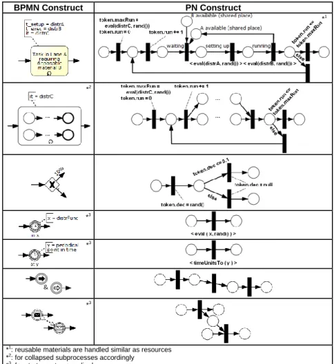
A single BPMN process can be transformed into a Petri net using the approach by Dijkman et al. [DDO08]. This approach is taken and extended here. Extensions are necessary in order to cover a) different execution states of an activity, b) required resources and materials, c) the existence of subprocesses, d) looping of activities and processes, e) execution durations and waiting times, f) branching probabilities, g) process links between diagrams, and h) communication between processes using messages.
Figure 4 shows all additional rules in order to extend Dijkman’s mapping for clinical pathway BPMN models. Thereby, the concept of a colored Petri net [Jen86] is used in order to store and query information in tokens which supports the covering of d) and f). Moreover for solving e), the Petri nets have to contain defined delays. Therefore, also the concept of timed Petri nets [Ram74] is picked up here: In timed Petri nets, constraints can be used in order to delay a transition’s firing after it becomes enabled for a certain time. In Figure 4, this time is denoted by<x>where x might be a function that has to be evaluated every time the transition becomes enabled by incoming token combinations.
to support colored tokens, time constraints on transitions as well as the four function rand()(providing a random number between 0 and 1),generateID()(providing an UUID),eval(d, n)(evaluating a distribution function d based on a number n) and timeUnitsTo(p)(calculating the duration to a periodic time p).
Time Mapper This utility maps qualified times defined in a process model and the
simulation parameters to time units used by the simulator. According to the requirements in Section 2.2, time values or time distributions can be either specified in seconds, minutes, hours, days or months. All these times are transformed into seconds when the Petri net is build, as the engine’s clock uses the smallest of these units. However, the resulting report should of course contain time values using the same units as specified in the model.
*2
BPMN Construct PN Construct
*1: reusable materials are handled similar as resources *2: for collapsed subprocesses accordingly
*3: for start events accordingly *3 *3 *3
*1
< timeUnitsTo (Monday) > < 10 min> < 30 min> < timeUnitsTo(6am) > < timeUnitsTo(8pm) > (a) (b) < timeUnitsTo (Saturday) > … token.id = generateID() token.id = generateID()
Figure 5: Rules for the integration of simulation parameters into the Petri net
For the transformation of periodic times (such as ’every morning at 7am’), the mapper needs to know when the simulation starts, which is specified in the simulation parameters. Using this information, a periodic time can be represented using the modulo operator: If a simulation for example starts at a certain date at midnight, ’every morning at 7am’ can be expressed byt≡(7·60·60) (mod24·60·60).
Simulation Parameter Integrator After transforming the BPMN diagrams into one
or several Petri nets, the simulation parameters need to be integrated. While the time mapper takes care about the simulation start and completion times, the frequency of process instantiations as well as the quantity of resources and materials have to be defined. If resources and materials are specified by constant values, only the specified number of tokens has to be put onto each shared resource/material place. If they vary over time (e.g., to specify different shift sizes), switching constructs have to be introduced.
In Figure 5 (a), a place is shown that represents a resource type with a staff size of three at day and two at night. A similar approach is taken in order to switch between different process instantiation frequencies (if specified). Figure 5 (b) shows that examplary for a process that starts every 10 min on working days and every 30 min on weekends. Please note, that (due to simplicity) the times within the diagrams have not been mapped to simulation time units.
Timed Petri Net Engine The generated and enriched Petri net can afterwards be executed
by the engine, which runs as long as the timer component advances the clock. The engine retrieves scheduled fire events and executes them along with subsequent firings that can be performed immediately. The firing of transitions that carry a time constraint is scheduled for a later point a time. During the course of a transition firing, new tokens are produced based on the incoming tokens and possibly defined transition rules. Also, each firing is logged. The following code listing shows the engine’s centralrun()method as well as its supporting recursivefire()method (all other supporting method are only named):
p u b l i c v o i d r u n ( ) {
w h i l e( t i m e r . a d v a n c e C l o c k ( ) )
f o r ( F i r e E v e n t e : t i m e . g e t S c h e d u l e d E v e n t s ( ) ) f i r e ( e . g e t T r a n s i t i o n ( ) , e . g e t T o k e n s ( ) ) ;
p r i v a t e v o i d f i r e ( T r a n s i t i o n t r a n s i t i o n , S e t<Token> t o k e n s ){ produceNewTokenToMarking ( t r a n s i t i o n , t o k e n s ) ; removeTokenFromMarking ( t o k e n s ) ; l o g ( t r a n s i t i o n , t o k e n s ) ; f o r ( P l a c e p : t r a n s i t i o n . g e t O u t g o i n g P l a c e s ( ) ) f o r ( T r a n s i t i o n t : p . g e t O u t g o i n g T r a n s i t i o n s ( ) ) i f ( ( S e t<Token> newTokens = i s N e w l y E n a b l e d ( t ) ) ! =n u l l) { i f ( t . c a n F i r e I m m e d i a t e l y ( ) ) f i r e ( t , newTokens ) ; e l s e { l o n g t i m e = 0 ; i f ( t . h a s P e r i o d i c T i m e ( ) ) t i m e = t i m e r . t i m e U n i t s T o ( t . g e t P e r i o d i c T i m e ( ) ) e l s e t i m e = t i m e r . g e t C u r r e n t T i m e ( ) + t i m e r . e v a l ( t . g e t D i s t r u t i o n F u n c t i o n ( ) , r a n d o m i z e r . r a n d ( ) ) ; t i m e r . s c h e d u l e ( t , newTokens ) ; } }
The JAVA code listing shows that firing of a transition only depends on its direct neighbors. For executing all possible firings at a certain time, not the whole net has to be traversed. Instead, we consider solely parts directly connected with transitions that are scheduled to fire at the current point in time. This optimizes the performance of the engine’s algorithm.
Timer As already shown, the timer manages the simulation clock and the calendar of
scheduled events. When requested by the engine, the timer advances the clock (as long as the simulation completion time is not reached) to the nearest scheduled time and returns all events associated with it. Moreover, the timer is responsible for the evaluation of time distribution functions (eval(d, n)) as well as the calculation of the duration to a periodic point in time (timeUnitsTo(p)).
eval(d, n)expects a functiondwith a domain of real numbers between 0 and 1. For an equal distribution between 20 to 100 time units,dcan be expressed byd(x) = 20 + 80x. Other possibilities fordinclude normal or exponential distributions but also manually defined ranges such as
d(x) = (
30, ifx <0.25 40, ifx≥0.25
As some of these functions produce real numbers but time values are represented by discrete natural numbers, the result of a function call might have to be rounded.
timeUnitsTo(p)expects an periodic timepexpressed using the modulo operator and returns the number of time units between the current time and the next occurrence of p. Ifpis defined byt ≡ x (mod y)andc denotes the current time, then we define timeUnitTo(p) { return modulo(x-c, y); } .
Randomizer This utility simply offers the generation of a random number between 0
and 1 by calling itsrand()method. Moreover, it provides agenerateID()method, generating an UUID based on random numbers. For both methods, the component relies on basic randomizer functionalities included in state-of-the-art programming languages.
Report Generator After completing the simulation, the report generator creates an Excel report based on the logged simulation events. Thereby, the logged events need to be transformed into performance measures on process-model level.
However, the simulation log only contains information about the firing of transitions. For each firing, the current time, the transition’s ID, and the produced tokens’ IDs are logged. Within the Excel report, these information need to be aggregated in order to obtain execution durations on activity-instance level (or event-instance level).
So, for each transition firing it has to be determined to which process instance it belongs and which activity-state (or event) was represented by the transition. This information can be encoded using the different IDs logged by the engine. Tokens on control flow places carry a process instance ID. Transition IDs on the other hand encode the ID of the represented activity and the state transition within the activity’s lifecycle.
After obtaining data on activity-instance level, it can be aggregated on different levels, for example for process instances, activity types and process definitions. Moreover they can be used in measures such as queue sizes and resource workload.
5
Conclusion
In this paper, we proposed an architecture blueprint for a business process simulation engine. We focused on the use case of simulating clinical pathways in a hospital. Based on the identified requirements, components of the architecture have been described in detail. In particular, we discussed how execution relevant annotations of a process model are considered during the simulation by leveraging timed and colored Petri nets.
As the next step, we plan to implement the simulation engine according to the presented architecture. Moreover, we plan to conduct a case study in order to evaluate our approach in a real world setting.
References
[BvMO08] Christian Bartsch, Marco von Mevius, and Andreas Oberweis. Simulation of IT Service Processes with Petri-Nets. InICSOC Workshops, volume 5472 ofLNCS, pages 53–65. Springer, 2008.
[DDO08] Remco M. Dijkman, Marlon Dumas, and Chun Ouyang. Semantics and analysis of business process models in BPMN.IST, 50(12):1281–1294, 2008.
[DJLN03] J¨org Desel, Gabriel Juh´as, Robert Lorenz, and Christian Neumair. Modelling and Validation with VipTool. InBPM, volume 2678 ofLNCS, pages 380–389. Springer, 2003.
[GS10] Christian Gierds and Jan S¨urmeli. Estimating costs of a service. InProceedings of the 2nd Central-European Workshop on Services and their Composition, ZEUS 2010, volume 563 ofCEUR Workshop Proceedings, pages 121–128. CEUR-WS.org, 2010.
[Jen86] Kurt Jensen. Coloured Petri Nets. InAdvances in Petri Nets, volume 254 ofLNCS, pages 248–299. Springer, 1986.
[JKW07] K. Jensen, L.M. Kristensen, and L. Wells. Coloured Petri Nets and CPN Tools for Modelling and Validation of Concurrent Systems. STTT, 9(3):213 – 254, May 2007. [KAMH09] Farzad Kamrani, Rassul Ayani, Farshad Moradi, and Gunnar Holm. Estimating
Per-formance of a Business Process Model. InProceedings of the 2009 Winter Simulation Conference, 2009.
[KLO08] Stefan Klink, Yu Li, and Andreas Oberweis. INCOME2010 - a toolset for developing process-oriented information systems based on petri nets. In S´andor Moln´ar, John Heath, Olivier Dalle, and Gabriel A. Wainer, editors,SimuTools, page 14. ICST, 2008. [MM07] Matteo Magnani and Danilo Montesi. BPMN: How Much Does It Cost? An Incremental
Approach. InBPM, volume 4714 ofLNCS, pages 80–87. Springer, 2007.
[omg09] Business Process Model and Notation (BPMN), Version 2.0 - Beta 1. Object Manage-ment Group (OMG), January 2009.
[Pet62] Carl Adam Petri. Communication with Automata (in German). PhD thesis, Universit¨at Bonn, Institut f¨ur Instrumentelle Mathematik, Schriften IIM Nr.2, 1962.
[PFKR10] Tomasz Porzucek, Mathias Fritzsche, Stephan Kluth, and David Redlich. Combina-tion of a Discrete Event SimulaCombina-tion and an Analytical Performance Analysis through Model-Transformations. InProceedings of the 17th IEEE International Conference and Workshop on the Engineering of Computer Based Systems, March 2010.
[PKCZ09] Tomasz Porzucek, Stephan Kluth, Flavius Copaciu, and Werner Zorn. Modeling and Evaluation Framework for FMC-QE. InProceedings of the 16th IEEE International Conference and Workshop on the Engineering of Computer Based Systems, 2009. [Ram74] C. Ramchandani. Analysis of Asynchronous Concurrent Systems by Timed Petri Nets.
Technical report, Cambridge, MA, USA, 1974.
[Ran80] Jorgen Randers.Elements of the System Dynamics Method. MIT Press, Cambridge, MA, USA, 1980.
[RWD+08] Changrui Ren, Wei Wang, Jin Dong, Hongwei Ding, Qinhua Wang, and Bing Shao. Towards a Flexible Business Process Modeling and Simulation Environment. In Pro-ceedings of the 2008 Winter Simulation Conference, 2008.
[SB08] Thomas J. Schriber and Daniel T. Brunner. Inside discrete-event simulation software: How it works and why it matters. InWinter Simulation Conference, pages 182–192, 2008.
[Swe99] Al Sweetser. A Comparison of System Dynamics (SD) and Discrete Event Simulation (DES). InInternational Conference of System Dynamics society and 5th Australian and Newzealand Systems Conference., 1999.
[TT07] Yifei Tan and Soemon Takakuwa. Predicting the Impact on Business Performance of Enhanced Information System Using Business Process Simulation. InProceedings of the 2009 Winter Simulation Conference, 2007.
[WJI09] K. Preston White Jr and Ricki G. Ingalls. Introduction to Simulation. InProceedings of the 2009 Winter Simulation Conference, 2009.
[WNW09] Gerd Wagner, Oana Nicolae, and Jens Werner. Extending Discrete Event Simulation by Adding an Activity Concept for Business Process Modeling and Simulation. In Proceedings of the 2009 Winter Simulation Conference, 2009.