(will be inserted by the editor)
Global and Decomposition Evolutionary Support Vector
Machine Approaches for Time Series Forecasting
Paulo Cortez · Juan Peralta Donate
Abstract Multi-step ahead Time Series Forecasting (TSF) is a key tool for support-ing tactical decisions (e.g., plannsupport-ing resources). Recently, the support vector machine emerged as a natural solution for TSF due to its nonlinear learning capabilities. This paper presents two novel Evolutionary Support Vector Machine (ESVM) methods for multi-step TSF. Both methods are based on an Estimation Distribution Algorithm (EDA) search engine that automatically performs a simultaneous variable (number of inputs) and model (hyperparameters) selection. The Global ESVM (GESVM) uses all past patterns to fit the support vector machine, while the Decomposition ESVM (DESVM) separates the series into trended and stationary effects, using a distinct ESVM to forecast each effect and then summing both predictions into a sin-gle response. Several experiments were held, using six time series. The proposed approaches were analyzed under two criteria and compared against a recent Evolu-tionary Artificial Neural Network (EANN) and two classical forecasting methods, Holt-Winters and ARIMA. Overall, the DESVM and GESVM obtained competitive and high quality results. Furthermore, both ESVM approaches consume much less computational effort when compared with EANN.
Keywords Estimation distribution algorithm·Support vector machines·Time series·Decomposition forecasting·Model selection
1 Introduction
Knowing what is more likely to happen in the future is a fundamental step for as-sisting modern-day decisions. Thus, building predictions based on historical data is a
ALGORITMI Research Centre, Department of Information Systems, University of Minho, Campus de Azur´em, 4800-058 Guimar˜aes, Portugal
E-mail: [email protected], http://www3.dsi.uminho.pt/pcortez Tel.: +351 253 510313 Fax: +351 253 510300
·Universidad Aut´onoma de Barcelona, Barcelona, Spain E-mail: [email protected]
key area of Information Technology [21]. Within this context, Time Series Forecast-ing (TSF) is an important prediction type, where the goal is to model the behavior of a given phenomenon (e.g., shoe sales) based on past patterns of the same event. TSF is becoming increasingly used in several scientific, industrial, commercial and economic activity areas [5]. In particular, multi-step ahead predictions (e.g., issued several months in advance) are useful to support tactical decisions, such as planning production resources, controlling stocks and elaborating budgets.
Due to its importance, several classical statistical methods were proposed for TSF, such as the popular Holt-Winters (HW), in the sixties [28] or Autoregressive Integrated Moving Average (ARIMA) model, in the seventies [2]. The HW is from the family of exponential smoothing methods and it based on the decomposition of a series into several components, such as trended and seasonal factors. The ARIMA model is based on a linear combination of past values (autoregressive component) and errors (moving average part). HW and ARIMA methods were developed decades ago, when higher computational restrictions prevailed (e.g., memory and computing power) and adopt rather fixed models (e.g., with multiplicative or additive seasonal-ity), that may not be suited when more complex patterns are present in the data.
More recently, modern prediction methods, such as Artificial Neural Networks (ANN) [18] (mid-eighties) and Support Vector Machines (SVM) [22] (mid-nineties) were proposed for TSF. These modern methods are natural solutions for TSF since they are more flexible (i.e., noa priorirestriction is imposed) when compared with classical TSF models, presenting learning capabilities that range from linear to com-plex nonlinear mappings. When compared with ANN, SVM presents theoretical ad-vantages. In particular, the SVM algorithm finds the optimal solution while the train-ing of ANNs (e.g., multilayer perceptrons) is sensitive to the choice of its initial weights. SVM is becoming a very popular data-driven method and recently it was considered one of the most influential data mining algorithms [30].
When adapting SVM to TSF, variable and model selection are critical issues [6][23][15]. Variable selection is useful to select the relevant time lags to be fed into the SVM. Moreover, SVM has several hyperparameters that need to be adjusted (e.g., kernel parameter) and thus model selection is important to avoid overfitting and to correctly adjust models to the implicit input-output mapping hidden within the data [13]. Ideally, variable and model selection should be performed simultaneously. Yet, most data mining applications tend to separate or overlook these issues [32].
To automate the design of the best forecasting model, performing a simultaneous variable and model selection, an interesting approach is to use evolutionary compu-tation [20], which performs a global multi-point (or beam) search, quickly locating areas of high quality, even when the search space is very large and complex. Most studies use evolutionary algorithms to optimize ANN models, known as Evolutionary ANN (EANN) [31][26][9][23][24]. Yet, with the increasing interest in SVM [30][3], Evolutionary SVM (ESVM) systems are also becoming popular [10, 16]. In all these studies, the major approach is to adopt the standard genetic algorithm [14], although there are more sophisticated search algorithms. The Estimation Distribution Algo-rithm (EDA), proposed in 2001 [19], makes use of exploitation and exploration prop-erties to find good solutions and outperformed in [9] the standard genetic algorithm and a differential evolution method when selecting the best ANN TSF models.
In this paper, we propose two novel ESVM approaches, both based on the EDA engine to automatically select the best SVM multi-step ahead forecasting model. The global ESVM (GESVM) approach performs a simultaneous search for the number of time lags and hyperparameters of the SVM and it is fit using all past patterns. Inspired by the classical forecasting methods (e.g., HW), the Decomposition ESVM (DESVM) approach first isolates the original series into trended and stationary (e.g., seasonal) effects. Next, it uses a ESVM to separately forecast each effect and then sums both predictions into a single response. Furthermore, we compare these two approaches with a recently proposed EANN [9] and also two popular TSF methods (HW and ARIMA), using two forecasting metrics and six time series from distinct domains and with different characteristics.
The paper is organized as follows. First, Section 2 describes the time series data, evaluation procedure and methods (GESVM, DESVM, EANN, HW and ARIMA). Then, in Section 3 we present the experimental setup and analyze the obtained results. Finally, we conclude the paper in Section 4.
2 Materials and Methods
2.1 Time Series Data
A time series is a collection of time ordered observationsy1,y2, ...,yt, each one
be-ing recorded at a specific time pointt[5]. A time series model ˆyt assumes that past
patterns will occur in the future. Thehorizon hdefines the time in advance that a pre-diction is issued. Multi-step ahead forecastsh∈ {1,2, ...,H}are often performed over monthly series and are used to support tactical decisions (e.g., planning production resources).
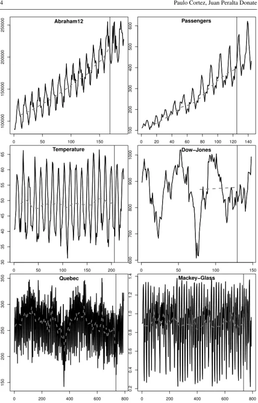
In this paper, we selected a set of six benchmark time series, with different char-acteristics and from distinct domains for the TSF evaluation (Table 1 and Figure 1). In this study, the first five datasets are related with real-world tasks and were selected from the Time Series Data Library (TSDL) repository [17], while the last chaotic series is described in [11]. It should be noted that these six times series were also adopted by theNN3andNN5forecasting competitions [8]. The real-world datasets are interesting to forecast since the data suffered from external and dynamic phe-nomena (e.g., weather changes, strikes, technological advances), which are difficult to predict and accurate forecasts can have an impact in their application domains. The Mackey-Glass series is often used to compare modern forecasting methods and has been chosen to extend the experimentation with a different benchmark, since it is not based on real data, not defined in terms of a timely period (e.g., daily or monthly) and contains no trend or noise components. Finally, we note that these time series were also studied in [9] for EANN, with similar splits into train (in-samples, column #train of Table 1) and test (out-of-samples, column #test) data, thus facilitating the comparison with EANN.
The autocorrelation coefficient is a useful tool to detect seasonal components or if a time series is random. It measures the correlation between a series and itself, lagged
0 50 100 150 100000 150000 200000 250000 Abraham12 0 20 40 60 80 100 120 140 100 200 300 400 500 600 Passengers 0 50 100 150 200 30 35 40 45 50 55 60 65 Temperature 0 50 100 150 600 700 800 900 1000 Dow−Jones 0 200 400 600 800 150 200 250 300 350 Quebec 0 200 400 600 800 0.2 0.4 0.6 0.8 1.0 1.2 1.4 Mackey−Glass
Fig. 1 Plots of the time series data (x-axis denotes the time periods,y−axis the data values, vertical line
Table 1 Time series data
Series Description (years) K#train #test
Abraham12 Monthly gasoline demand in Ontario (1960-75) 12 168 24 Passengers Monthly international airline passengers (1949-60) 12 125 19 Temperature Mean monthly air temp. Nottingham Castle (1920-39) 12 206 19 Dow-Jones Monthly closings of the Dow-Jones index (1968-81) 50 129 19 Quebec Daily number of births in Quebec (1977-78) 7 735 56 Mackey-Glass Mackey-glass chaotic series 17 735 56
ofkperiods, and can be computed by [2]:
rk=∑
P−k
t=1(yt−y)(yt+k−y)
∑Pt=1(yt−y)2
(1)
wherey1,y2, ...,yPstands for the time series,Pfor the current time period (column
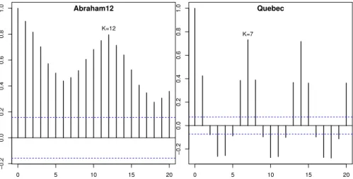
#train from Table 1), andyfor the series average. Figure 2 shows examples of auto-correlations for Abraham12 (left) and Quebec (right). In the plots, the seasonal period
Kis clearly visible. Also, severalrkvalues are above the 95% degree of confidence
normal distribution bounds (horizontal dashed lines), showing that these series are not random and thus can be predicted. To automatically detect the seasonal period
K, we adopt in this study an autocorrelation-based heuristic rule, which consists in finding the first maximumrkvalue such thatrk>rk−1andrk>rk+1. The columnK
of Table 1 presents the results of applying such rule when using only training data.
0 5 10 15 20 −0.2 0.0 0.2 0.4 0.6 0.8 1.0 Abraham12 K=12 0 5 10 15 20 −0.2 0.0 0.2 0.4 0.6 0.8 1.0 Quebec K=7
Fig. 2 Autocorrelations (rkvalues,y-axis) for Abraham12 and Quebec series (using only training data;
2.2 Evaluation
The global performance of a forecasting model is evaluated by an accuracy measure, such as Mean Squared Error (MSE), Relative Squared Error (RSE) and Symmetric Mean Absolute Percentage Error (SMAPE):
MSE =H1∑tP=+PH+1et2 RSE = ∑ P+H t=P+1e2t ∑tP=+PH+1(yt−y)2 ×100% SMAPE =H1∑tP=+PH+1 |et| (|yt|+|yˆt|)/2×100% (2)
whereet=yt−yˆtdenotes the forecasting error at timet. andHis the maximum
fore-casting horizon (column #test from Table 1). In all MSE, RSE and SMAPE metrics, lower values denote better forecasts. However, RSE and SMAPE have the advantage of being scale independent and thus can be used to compare results across different series. RSE is a relative-based metric, where a value lower than 100% shows that the forecasting model is better than predicting always the average of the test data values. RSE and MSE have been widely used in the forecasting domain [29]. SMAPE is a percentage error metric that can be directly understood by domain users. We adopt the variant used in [1], since it does not lead to negative values, thus ranging from 0% to 200%. SMAPE was also the error metric used inNN3,NN5andNNGC1 forecast-ing competitions [8]. Squared error based metrics, such as RSE, are more sensitive to outliers when compared with absolute error based metrics, such as SMAPE. For performing a correct evaluation, we opt for computing both measures over the test samples of Table 1. To aggregate results over all time series, we calculate both mean and median values. We note that the latter measure is less sensitive to outliers, making the global evaluation of the results not dependent of a good result in just one series.
2.3 Evolutionary Support Vector Machine
Any regression algorithm (e.g., SVM) can be applied to TSF by adopting a sliding time window, which is defined by the set of time lags{1,2, ...,I}used to build a fore-cast [6]. For a time periodt, the model inputs areyt−I, ...,yt−2,yt−1and the desired
output isyt. For example, let us consider the series 61,102,143,184,235(yt values).
If the sliding window{1,2,3}is adopted, then two training examples can be cre-ated: 6,10,14→18 and 10,14,18→23. After training, the last known values are fed into the model and multi-step forecasts are built by iteratively using 1-step ahead predictions as inputs.
Before fitting the SVM models, the data are normalized into the range[0,1], using maximum and minimum values computed over training data only, and once the model outputs the resulting values, the inverse process is carried out, rescaling them back to the original scale [13]. The training data is used to train and validate each model generated during the evolutionary execution, thus it is split into two subsets, training (with the first 70% elements of the series) and validation (with the remaining ones), under a timely ordered holdout scheme.
When designing a SVM model, there are three crucial issues that should be taken into account: the type of SVM to use, the selection of the kernel function and tuning the parameters associated with the two previous selections. Since TSF is a particular regression case, for the SVM type and kernel, we selected the pop-ularε-insensitive loss function (known asε-SVR) and Gaussian kernel (κ(x,x0) = exp(−λ||x−x0||2),λ>0) combination, as implemented in theLIBSVMtool [4]. In
SVM regression [27], the inputy= (yt−I, ...,yt−2,yt−1), for a SVM withIinputs, is
transformed into a highm-dimensional feature space, by using a nonlinear mapping
φ that does not need to be explicitly known but that depends on a kernel function.
Then, the SVM algorithm finds the best linear separating hyperplane, tolerating a small errorεwhen fitting the data, in the feature space:
ˆ yt=w0+ m
∑
j=1 wjφj(y) (3)The SVM performance is affected by three parameters:λ,εandC(a trade-off
be-tween fitting the errors and the flatness of the mapping).
In this paper, an evolving hybrid system that uses EDA and SVM, is proposed. Following the suggestion of theLIBSVMauthors [4], SVM parameters are searched in terms an exponentially growing scale. We also take into account the number of time lags or inputsI used to train the SVM. Therefore, we adopt a direct encoding scheme, using a numeric representation with 8 genes, according to the chromosome
g1g2g3g4g5g6g7g8, such that: I =10g1+g2+1,g1∈ {0,1, ...,9}andg1∈ {0,1, ...,9} γ =2(g3+g104)−5 ,g3∈ {−9,−8, ...,9}andg4∈ {−9,−8, ...,9} C=2(g5+ g6 10)+5 ,g5∈ {−9,−8, ...,9}andg6∈ {−9,−8, ...,9} ε =2(g7+g108)−8 ,g7∈ {−9,−8, ...,9}andg8∈ {−9,−8, ...,9} (4)
wheregi denotes thei-th gene of the chromosome. Thus, the ranges for the search
space are:I∈ {1,2, ...,100};γ∈2[−14.9,4.9];C∈2[−4.9,14.9]; andε∈2[−17.9,1.9].
The ESVM process consists of the following steps:
1. First, a randomly generated population (composed of to 50 individuals), i.e., a set of randomly generated chromosomes, is obtained.
2. The phenotypes (SVM model) and fitness value of each individual of the actual generation is obtained. This includes the steps:
(a) The phenotype of an individual of the actual generation is first obtained (using
LIBSVM[4]).
(b) The training data is divided into training and validation subsets.
(c) The model is fitted using the Sequential Minimal Optimization algorithm, as implemented inLIBSVM. The fitness for each individual is given by the MSE during the learning process. The aim is to reduce extreme errors (e.g., outliers) that can highly affect multi-step ahead forecasts. Moreover, prelim-inary experiments (with time series not present in Table 1), have shown that this choice leads to better forecasts when compared with absolute errors.
3. Once the fitness values for whole population have been already obtained, UMDA-EDA (with no dependencies between variables) [9] operators (selection, estima-tion of the empirical probability distribuestima-tion and sampling soluestima-tions) are applied in order to generate the population of the next generation, i.e., a new set of chro-mosomes.
4. Steps 2 and 3 are iteratively executed until a maximum number of generations is reached.
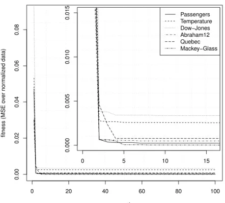
The parameters of the EDA (e.g., population size of 50) were set to the same values used by the EANN proposed in [9]. Since the EDA works as a second order optimiza-tion procedure, the tuning of its internal parameters is not a critical issue (e.g., using a population of 48 does not substantially change the results). Also, this EDA has a fast convergence (shown in Figure 3), quickly reaching a stable fitness value.
Fig. 3 Evolution of the GESVM best fitness value for all series (with a bottom left zoom).
0 20 40 60 80 100 0.00 0.02 0.04 0.06 0.08 generations fitness (MSE o ver nor maliz ed data) 0 5 10 15 0.000 0.005 0.010 0.015 PassengersTemperature Dow−Jones Abraham12 Quebec Mackey−Glass
2.4 Decomposition Based Evolutionary Support Vector Machine
In classical decomposition forecasting (e.g., HW), distinct components such as trend and seasonal effects are first isolated and then predicted independently. Inspired by this concept, we propose a novel DESVM approach for TSF. The rationale is that it might be better to perform a specialization, where a distinct SVM will capture the trend and stationary components. The focus is set in terms of separating the trend, since this is a strong component that often obscures other interesting patterns, such as seasonal effects. For instance, the ARIMA methodology first removes trend from a time series in order to accurately perform the model identification [2].
The proposed DESVM works as follows. First, the original time seriesytis
trans-formed into two series:Tt andSt, corresponding to its trend and stationary
compo-nents. To estimate the trend series, we propose a heuristic that requires knowing the seasonal periodKin advance in order to average all values within a given seasonal period:
Tl=yi,i∈ {l−K+1,l−K+2, ...,l} (5)
wherel∈L,L={PmodK+K, ...,P−2K,P−K,P}. The remainingTj values are
computed by interpolating a line between two consecutiveTl1,Tl2 elements (l1,l2∈ L). The estimated trends for the series of Table 1 are plotted with dashed gray lines in Figure 1. The plots make clear that for strong trended series, such as Passengers and Abraham12, the estimated trend values capture well the implicit trend. Regarding the stationary component, it is simply defined as St =yt−Tt. Next, each
individ-ual decomposed series is modeled using a distinct ESVM, which works as defined in Section 2.3. After executing both ESVM systems, the final prediction is built by combining the individual responses:
ˆ
yt=Tˆt+Sˆt,t∈ {P+1, ...,P+H} (6)
where ˆTtand ˆStdenote the predicted trend and stationary components at timet.
2.5 Evolutionary Artificial Neural Network
For the comparison, we have chosen a recently proposed EANN [9], which is similar to ESVM (e.g., use of EDA, fitness based on MSE) except that is uses a fully con-nected multilayer perceptron, with one hidden layer and logistic activation functions. This base learner is trained with the RPROP algorithm, as implemented using the
SNNStool [33]. EANN optimizes the number of inputs (I∈ {1, ...,100}), ANN hid-den nodes (from 0 to 99) and the RPROP parameters (∆0∈ {1,0.01,0.001, ...,10−9}
2.6 Holt-Winters
HW is based trend and seasonal patterns that are distinguished from random noise by averaging the historical values [28]. The multiplicative model is defined by:
Level Bt=αDt−Kyt + (1−α)(Bt−1+Et−1) Trend Et=β(Bt−Bt−1) + (1−β)Et−1 SeasonalityDt=γByt t + (1−γ)Dt−K ˆ yt+i,t= (Bt+iEt)×Dt−K+i (7)
whereBt,Et andDt denote the level, trend and seasonal estimates and α, β and γ are the model parameters. To optimize the HW parameters, we adopt a 0.05 grid
search for the best training error (MSE), which is a common procedure within the forecasting field. The HW was implemented using thestats package of the open-sourceRstatistical tool [25].
2.7 ARIMA method
When compared with HW, ARIMA often presents an higher accuracy over a wider domain of series. Several ARIMA variants can be defined, each based on a linear combination of past values (AR components) and errors (MA part). For example, the seasonal version is denoted by the termARIMA(p,d,q)(P1,D1,Q1)and can be
written as: φp(L)ΦP1(L K)(1−L)d(1−L)D1y t=θq(L)ΘQ1(L K)e t (8)
whereΦP1 andΘQ1 are polynomial functions of ordersP1andQ1.
The order and coefficients of the model are usually estimated by statistical ap-proaches (e.g., least squares methods). To get the ARIMA forecasts, we adopted the automatic selection of the commercialForecastProc tool [12]. The rationale is to use a popular benchmark that can easily be compared and that does not require ex-pert model selection capabilities from the user. The automatic procedure includes the search for the best ARIMA model, its internal coefficients, and detection of events such as level shifts or outliers, thus this benchmark is difficult to outperform.
3 Results
The two ESVM approaches and EANN experiments were conducted using code writ-ten in theClanguage by the authors. In the experiments, we used a maximum of 100 generations as the stopping criterion for the EDA search engine. The forecasting met-ric results are shown in Table 2.
When analyzing Table 2, DESVM stands out as the best forecasting method. For both error metrics, DESVM outperforms other approaches in 3 (Abraham12, Dow-Jones and Quebec) of the 6 series and also obtains the best aggregate (i.e., mean and
Table 2 Forecasting errors (%RSE and %SMAPE, best values inbold).
Error Time Series HW ARIMA EANN GESVM DESVM
%RSE Abraham12 70.75 53.39 35.34 35.67 17.34 Passengers 5.43 9.16 7.93 16.18 12.04 Temperature 7.27 6.67 6.66 10.81 8.50 Dow-Jones 147.02 108.68 166.74 145.25 108.64 Quebec 82.87 73.42 99.26 69.61 59.46 Mackey-Glass 166.90 96.91 7.40 1.23 2.40 Mean 80.04 58.04 53.89 46.46 34.73 Median 76.81 63.41 21.63 25.93 14.69 %SMAPE Abraham12 6.70 6.21 4.71 4.87 3.45 Passengers 3.28 4.51 3.39 5.35 4.86 Temperature 3.74 3.42 3.51 4.43 3.85 Dow-Jones 6.39 4.78 6.28 6.36 4.64 Quebec 11.01 10.37 10.83 9.46 9.39 Mackey-Glass 33.78 26.94 7.07 3.25 4.33 Mean 10.82 9.37 5.97 5.62 5.08 Median 6.55 5.50 5.50 5.11 4.48
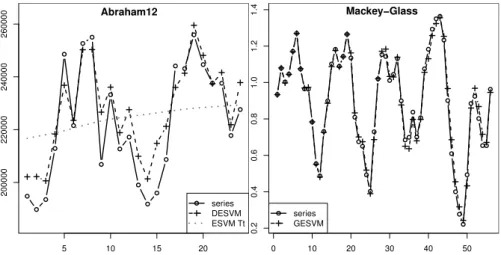
median) results. The remaining approaches rank first only for one series: HW for Pas-sengers (RSE and SMAPE), ARIMA for Temperature (SMAPE), EANN for Temper-ature (RSE) and GESVM for Mackey-Glass (RSE and SMAPE). Overall, considering both mean and median aggregate measures, GESVM is the second best method, fol-lowed by EANN (third place), ARIMA (fourth) and HW (fifth). The two exceptions are for: RSE and median (EANN is ranked at second place); and SMAPE and median (ARIMA and EANN tie at third place). To demonstrate the quality of the obtained forecasts, Figure 4 plots the DESVM results (estimated trend ˆTtand combined
fore-cast ˆyt) for Abraham 12 and GESVM forecasts for Mackey-Glass. In both cases, a
high quality fit was achieved.
5 10 15 20 200000 220000 240000 260000 Abraham12 series DESVM ESVM Tt 0 10 20 30 40 50 0.2 0.4 0.6 0.8 1.0 1.2 1.4 Mackey−Glass series GESVM
Fig. 4 Forecasts for DESVM and Abraham12 (left) and GESVM and Mackey-Glass (right), wherex-axis
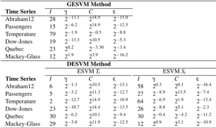
Table 3 Best GESVM and DESVM forecasting models GESVM Method Time Series I γ C ε Abraham12 28 2−13.1 214.9 2−15.0 Passengers 15 2−6.2 214.9 2−12.5 Temperature 79 2−1.9 2−0.5 2−8.8 Dow-Jones 19 2−13.3 210.5 2−5.3 Quebec 23 20.2 2−3.30 2−3.4 Mackey-Glass 12 21.9 23.9 2−16.2 DESVM Method ESVMTt ESVMSt Time Series I γ C ε I γ C ε Abraham12 6 2−1.3 210.5 2−13.1 58 20.3 20.1 2−16.4 Passengers 5 2−3.2 211.3 2−12.7 27 2−8.9 213.5 2−7.4 Temperature 2 2−12.7 214.9 2−16.9 64 2−6.9 21.8 2−13.4 Dow-Jones 23 2−10.7 214.4 2−13.5 26 2−8.8 25.1 2−2.3 Quebec 30 2−6.2 210.1 2−9.4 30 2−0.4 2−4.2 2−11.2 Mackey-Glass 29 2−3.8 211.9 2−12.5 12 20.9 23.1 2−10.9
The best forecasting models for GESVM and DESVM are presented in Table 3, each model defined in terms of its number of inputs I and hyperparameters γ,C
andε. For the first three series (Abraham12, Passengers and Temperature), DESVM
optimized individual SVMs that are quite distinct in terms of the number of inputs, confirming the specialization performed by each SVM. Moreover, the GESVM and ESVMStmodels have a number of inputs that includes the adopted seasonal period
(Kfrom Table 1), except for Dow-Jones and Mackey-Glass, which do not contain a clear and fixed seasonal cycle. For Mackey-Glass, GESVM and ESVMStmodels are
quite similar. This result makes sense since Mackey-Glass is a stationary series and thus the trended ESVM component not particularly relevant.
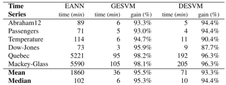
The experimentation was carried out with an exclusive access to a server (Intel Xeon 2.27 GHz processor using Linux). Table 4 shows the computational time (in minutes) required by each evolutionary method. The two gain columns show (in %), the reduction of computational effort obtained by GESVM and DESVM when com-pared with EANN, which is measured as 1−(tM/tEANN), wheretMandtEANNdenote
the computational times required for methodsM∈ {GESV M,DESV M}and EANN. As shown by the table, GESVM and DESVM demand much less computational effort when compared with EANN, presenting an overall gain that is higher than 90%. Over-all, when analyzing mean and median measures, DESVM requires around twice the computation of the global ESVM (as expected). Nevertheless, we noted that DESVM can be easily parallelized by running each of its two ESVM components in a different processor or core.
Classical methods are fast enough. Alternative approaches such as EANN pro-vide slightly better accuracy but are too time consuming, since they cannot be used for quick predictions of high frequency time series. Even in case of larger frequen-cies (e.g., monthly), users usually do not want to wait tens or hundreds of minutes. Hence, we provide a new approach that is even more precise than EANN and that is much faster. Although it does not reach the speed of classical approaches, the time
requirements are not that much limiting, which may be found as a confirmation of the promising approach we suggest.
Table 4 Comparison of computational effort required by EANN, GESVM and DESVM.
Time EANN GESVM DESVM
Series time (min) time (min) gain (%) time (min) gain (%)
Abraham12 89 6 93.3% 5 94.4% Passengers 71 5 93.0% 4 94.4% Temperature 114 6 94.7% 11 90.4% Dow-Jones 73 3 95.9% 9 87.7% Quebec 5221 95 98.2% 192 96.3% Mackey-Glass 5590 105 98.1% 205 96.3% Mean 1860 36 95.5% 71 93.3% Median 102 6 95.3% 10 94.4% 4 Conclusions
Forecasting the future based on past data is a key issue to support decision mak-ing in a wide range domains, includmak-ing scientific, industrial, commercial and eco-nomic activity areas. In this paper, we address multi-step ahead Time Series Forecast-ing (TSF), which is useful to support tactical decisions, such as plannForecast-ing resources, stocks and budgets. As the base learner, we adopt the modern Support Vector Machine (SVM), which often achieves high quality predictive results and presents theoretical advantages (e.g., optimum learning convergence) over other learners, such as Artifi-cial Neural Networks (ANN). To automate the search of the best SVM forecasting model, we use a recently proposed evolutionary algorithm: Estimation Distribution Algorithm (EDA). This search method is used to perform a simultaneous variable (number of inputs) and model (hyperparameters) selection. Using EDA, we propose two Evolutionary SVM (ESVM) variants for TSF, under global (GESVM) and de-composition (DESVM) approaches. The former uses all past patterns to fit the SVM, while the latter decomposes first the original series into trended and stationary com-ponents, then uses ESVM to predict each individual component and finally sums both predictions to get the global response.
The two ESVM variants were compared over six distinct time series and under two criteria (RSE and SMAPE). For comparison purposes, we also tested a recent Evolutionary EANN (EANN) [9] and two popular classical methods, Holt-Winters (HW) and Autoregressive Integrated Moving Average (ARIMA). Under the tested setup (time series, forecasting horizons, error metrics), the results show a competi-tive behavior of the proposed approaches. Overall, when considering both mean and median over all series, DESVM is best choice, followed by GESVM (second best method), EANN (ranked third), ARIMA (fourth) and HW (fifth). Indeed, high qual-ity forecasting results were achieved (e.g., 4.5% and 5.1% median SMAPE values for DESVM and GESVM). These results are highlighted by the fact that we perform
a multi-step ahead forecasting, which is more difficult than one-step ahead predic-tion (such as studied in [7]). Moreover, the proposed ESVM methods can quickly obtain accurate forecasts, requiring much less computational effort when compared with EANN, with a reduction higher than 90%.
Both ESVM approaches are general purpose TSF methods that can be applied to a time series with few or noa prioriknowledge. Thus, DESVM and GESVM are suited for non specialized users. GESVM is a totally automatic method, while DESVM re-quires the setting of one parameter, the seasonal periodK, for creating the estimated trend component. Nevertheless, we stress that quite often such parameter is known by the user (e.g., in monthly sales typicallyK=12). Another alternative is the use of heuristics, such as the autocorrelation rule adopted in this paper. DESVM was de-signed for series with trend components and thus it naturally achieved better results for series with a strong trend (e.g., Abraham12 and Passengers), and worst results for Mackey-Glass (stationary series), when compared with GESVM. While DESVM still achieved good results for moderate or no trend series (e.g., Temperature), a spe-cialized user could use a trend detection method over the training data (e.g., visual inspection, use of autocorrelations) to opt between DESVM and GESVM. In addi-tion, we would like to stress that DESVM provides more predictive information than GESVM (expected future trend and stationary patterns), which might be useful in some real-world applications (e.g., to know if there is a steady increase in sales be-hind the normal seasonal pattern).
In the future, we intend to extend the ESVM approaches for multivariate time se-ries, which are common in the economic domain (e.g., financial markets) and address other SVM kernels (e.g., Polynomial and Spline). Also, we intend to adapt and test the proposed methods for time series with multiplicative decomposition components (rather than just additive) and with two or more seasonal components (e.g., due to daily and weekly effects).
Acknowledgments
The authors wish to thank Ramon Sagarna for introducing the subject of EDA. The work of P. Cortez was supported by FEDER (program COMPETE and FCT) under project FCOMP-01-0124-FEDER-022674.
References
1. Andrawis, R., Atiya, A.: A new Bayesian formulation for Holt’s exponential smoothing. Journal of Forecasting28(3), 218–234 (2009)
2. Box, G., Jenkins, G.: Time Series Analysis: Forecasting and Control. Holden Day, San Francisco, USA (1976)
3. Camastra, F., Filippone, M.: A comparative evaluation of nonlinear dynamics methods for time series prediction. Neural Computing and Applications18(8), 1021–1029 (2009)
4. Chang, C.C., Lin, C.J.: LIBSVM: A library for support vector machines. ACM Transactions on Intelligent Systems and Technology2, 27:1–27:27 (2011)
6. Cortez, P.: Sensitivity Analysis for Time Lag Selection to Forecast Seasonal Time Series using Neural Networks and Support Vector Machines. In: Proceedings of the International Joint Conference on Neural Networks (IJCNN 2010), pp. 3694–3701. IEEE, Barcelona, Spain (2010)
7. Cortez, P., Rio, M., Rocha, M., Sousa, P.: Multi-scale internet traffic forecasting using neural networks and time series methods. Expert Systems29(2), 143–155 (2012)
8. Crone, S.: Time series forecasting competition for neural networks and computational intelligence. http://www.neural-forecastingcompetition.com (Accessed on January, 2011)
9. Donate, J., Li, X., S´anchez, G., de Miguel, A.: Time series forecasting by evolving artificial neu-ral networks with genetic algorithms, differential evolution and estimation of distribution algorithm. Neural Computing and Applications22(1), 11–20 (2013)
10. Feng, X., Zhao, H., Li, S.: Modeling non-linear displacement time series of geo-materials using evolu-tionary support vector machines. International journal of rock mechanics and mining sciences41(7), 1087–1107 (2004)
11. Glass, L., Mackey, M.: Oscillation and chaos in physiological control systems. Science197, 287–289 (1977)
12. Goodrich, R.L.: The Forecast Pro methodology. International Journal of Forecasting16(4), 533–535 (2000)
13. Hastie, T., Tibshirani, R., Friedman, J.: The Elements of Statistical Learning: Data Mining, Inference, and Prediction. Springer-Verlag, NY, USA (2008)
14. Holland, J.: Adaptation in natural and artificial systems. Ph.D. thesis, University of Michigan, Ann Arbor (1975)
15. Hsu, C.M.: A hybrid procedure with feature selection for resolving stock/futures price forecasting problems. Neural Computing and Applications22(3-4), 651–671 (2013)
16. Huang, H., Chang, F.: Esvm: Evolutionary support vector machine for automatic feature selection and classification of microarray data. Biosystems90(2), 516–528 (2007)
17. Hyndman, R.: Time Series Data Library. http://datamarket.com/data/list/?q=provider: tsdl(January, 2013)
18. Lapedes, A., Farber, R.: Non-Linear Signal Processing Using Neural Networks: Prediction and Sys-tem Modelling. Technical Report LA-UR-87-2662, Los Alamos National Laboratory, USA (1987) 19. Larranaga, P., Lozano, J.: Estimation of Distribution Algorithms: A New Tool for Evolutionary
Com-putation (Genetic Algorithms and Evolutionary ComCom-putation). Springer (2001) 20. Michalewicz, Z., Fogel, D.: How to solve it: modern heuristics. Springer (2004)
21. Michalewicz, Z., Schmidt, M., Michalewicz, M., Chiriac, C.: Adaptive Business Intelligence. Springer (2006)
22. Miiller, K., Smola, A., Ratsch, G., Scholkopf, B., Kohlmorgen, J., Vapnik, V.: Predicting time series with support vector machines. In: Proc. of the 7th Int. Conference on Artificial Neural Networks, pp. 999–1004. Springer (1997)
23. Parras-Gutierrez, E., Rivas, M.G.A.V., del Jesus, M.: Coevolution of lags and rbfns for time series forecasting: L-co-r algorithm. Soft Computing16(6), 919–942 (2012)
24. Parras-Gutierrez, E., Rivas, V., M. Garcia-Arenas, M.d.: Short, medium and long term forecasting of time series using the l-co-r algorithm. Neurocomputing128, 433–446 (2014)
25. R Core Team: R: A Language and Environment for Statistical Computing. R Foundation for Statistical Computing, Vienna, Austria (2013). ISBN 3-900051-07-0,http://www.R-project.org
26. Rocha, M., Cortez, P., Neves, J.: Evolution of Neural Networks for Classification and Regression. Neurocomputing70, 2809–2816 (2007)
27. Smola, A., Sch¨olkopf, B.: A tutorial on support vector regression. Statistics and Computing14, 199– 222 (2004)
28. Winters, P.R.: Forecasting sales by exponentially weighted moving averages. Management Science6, 324–342 (1960)
29. Witten, I., Frank, E.: Data Mining: Practical Machine Learning Tools and Techniques with Java Im-plementations. Morgan Kaufmann, San Francisco, CA (2005)
30. Wu, X., Kumar, V., Quinlan, J.R., Ghosh, J., Yang, Q., Motoda, H., McLachlan, G.J., Ng, A.F.M., Liu, B., Yu, P.S., Zhou, Z.H., Steinbach, M., Hand, D.J., Steinberg, D.: Top 10 algorithms in data mining. Knowledge and Information Systems14(1), 1–37 (2008)
31. Yao, X.: Evolving artificial neural networks. Proceedings of the IEEE87(9), 1423–1447 (1999) 32. Yu, M., Shanker, M., Zhang, G., Hung, M.: Modeling consumer situational choice of long distance
33. Zell, A., Mamier, G., H¨ubner, R., Schmalzl, N., Sommer, T., Vogt, M.: Snns: An efficient simulator for neural nets. In: MASCOTS ’93: Proceedings of the International Workshop on Modeling, Analysis, and Simulation On Computer and Telecommunication Systems, pp. 343–346. Society for Computer Simulation International, San Diego, CA, USA (1993)