Induction of comprehensible models for gene expression datasets by subgroup discovery methodology

Induction of comprehensible models for gene expression datasets

by subgroup discovery methodology

Dragan Gamberger

, Nada Lavracˇ

, Filip Z

ˇ elezny´

, Jakub Tolar

c_{Nova Gorica Polytechnic Vipavska 13, 5000 Nova Gorica, Slovenia}

d_{Department of Cybernetics, Czech Institute of Technology (CVUT FEL), Technicka´ 2, 16627 Prague, Czech Republic} e_{Department of Biostatistics, University of Wisconsin Medical School, 1300 University Avenue, 53706 Madison, USA} f_{Institute of Human Genetics, University of Minnesota Medical School, 420 Delaware Street, 55455 Minneapolis, USA}

Received 14 June 2004

Abstract

Finding disease markers (classifiers) from gene expression data by machine learning algorithms is characterized by a high risk of overfitting the data due the abundance of attributes (simultaneously measured gene expression values) and shortage of available examples (observations). To avoid this pitfall and achieve predictor robustness, state-of-the-art approaches construct complex clas-sifiers that combine relatively weak contributions of up to thousands of genes (attributes) to classify a disease. The complexity of such classifiers limits their transparency and consequently the biological insights they can provide. The goal of this study is to apply to this domain the methodology of constructing simple yet robust logic-based classifiers amenable to direct expert interpretation. On two well-known, publicly available gene expression classification problems, the paper shows the feasibility of this approach, employ-ing a recently developed subgroup discovery methodology. Some of the discovered classifiers allow for novel biological interpretations.

2004 Elsevier Inc. All rights reserved.

Keywords:Gene expression measurements; Disease markers; Subgroup discovery; Machine learning; Comprehensible classification

1. Introduction

Gene expression monitoring by DNA microarrays (gene chips) provides an important source of informa-tion that can help in understanding many biological pro-cesses. This technology allows for novel applications, resulting in increased understanding of disease pro-cesses, and improved diagnosis and prediction in medicine.

Data collected in these applications are not suitable for direct human explanatory analysis because a single DNA microarray experiment results in thousands of measured expression values and also because of the lack of existing expert knowledge available for the analysis. The application of various data mining and knowledge discovery methods using machine learning algorithms [39] seems an evident approach to take in such a prob-lem domain. Numerous approaches have been suggested towards exploiting state-of-the-art machine learning or microarray data mining, including both supervised learning (learning from data with class labels) and unsu-pervised learning (such as conceptual clustering). A state-of-the-art review of these various approaches can be found in[15,40].

1532-0464/$ - see front matter 2004 Elsevier Inc. All rights reserved. doi:10.1016/j.jbi.2004.07.007

*_{Corresponding author. Fax: +385 1 4680 114.}

E-mail addresses: [email protected] (D. Gamberger),

[email protected](N. Lavracˇ),[email protected], zelezny@biostat.

wisc.edu (F. Zˇ elezny´),[email protected](J. Tolar).

In this study, we follow the supervised learning para-digm. The database we analyze consists of a set of gene expression measurements (examples), each correspond-ing to a rather large number of measured expression val-ues of a predefined family of genes (attributes). Each measurement in the database was extracted from a tissue of a patient with a specific disease; this disease is the class for the given example. The standard goal of ma-chine learning is to start from such available labeled examples and construct classifiers that can successfully classify new, previously unseen examples. Such classifi-ers are important because they can be used for diagnos-tic purposes in medicine and because they can help to understand the dependencies between classes (diseases) and attributes (gene expression values).

The problem of finding disease markers (classifiers) from gene expression data by machine learning algo-rithms is characterized by the abundance of attributes (simultaneously measured gene expression values), and the shortage of the available examples (patients subject to measurements). The application of machine learning algorithms in a domain characterized by a large number of attributes typically calls for some dimensionality reduction, even if the employed strategy can in principle directly accept all the available attribute values. The ben-efits of prior elimination of irrelevant (or weakly relevant) attributes in data preprocessing has been recognized in machine learning[35]: besides helping to reduce the prob-lem complexity and the computation time, it can enable the construction of more accurate classifiers.

From the dimensionality point of view, the gene expression domain is specifically unfavorable, because— as we have mentioned—the abundance of attributes is confronted with a relatively small number of available examples. It is known from the machine learning and sci-entific discovery literature that such domains are prone to overfitting: overfitted classifiers are characterized by sig-nificantly decreased predictive accuracy on unseen sam-ples compared to the training set accuracy, or—in other words—by a high generalization error [14]. See[21] for an extensive treatment of different effects of overfitting. Informally, in domains characterized by a small number of examples and a large number of attributes, overfitting occurs because some artifacts (flukes) of actually irrele-vant attribute combinations can emerge simply by means of chance and appear significant with respect to the exam-ples available to a machine learning algorithm.

To avoid the overfitting pitfall, state-of-the-art ap-proaches construct complex classifiers that combine rel-atively weak contributions of up to thousands of genes (attributes) to classify a disease [20,45,10,36]. Predictor robustness is achieved by the redundancy of classifiers, realized, e.g., by voting of multiple classifiers. For exam-ple, [20] use weighted voting of informative genes,

[45,10]employ the support vector machine (SVM)

para-digm, while in [36] scores of top ranked emerging

pat-terns are used. The achieved prediction quality on independent test sets are very high but a drawback of classifiers based on many attributes is that they are not appropriate for expert interpretation. Although it is pos-sible to extract the attributes with maximal voting weight (in [45] such genes are called disease markers and some of them are already identified as useful in rou-tine clinical practice), the logical connections among the extracted attributes are lost and the construction of ex-pert comprehensible (disease) models remains a very dif-ficult task.

This paper describes an approach to the detection of rules for the classes of gene expression samples that are much more convenient for expert interpretation, taking gene expression data modeling as a novel challenge for the application of the recently developed subgroup dis-covery methodology [19]. Its goal is the induction of classifiers in the form of explicit short rules describing important subgroups of the target class samples, although these simple classifiers may be of a lower pre-dictive quality than the more complex classifiers. In-duced rules typically include 2–5 gene expression attributes and, in contrast to markers obtained from voting schemes, these rules explicitly stress the impor-tance of the correlation of the activity (or non-activity) of genes in the selected set of attributes. The problem with the induction of low dimensional, non-redundant classifiers is that they are prone to overfitting the train-ing set. The selection of an appropriate hypothesis lan-guage as well as the reduction of the hypothesis search space are known methods for avoiding overfitting [46]. Handling overfitting by relevancy based feature and rule filtering are important aspects of this work. In rule learning, the problem of this approach is that with a strongly reduced hypothesis space it may be difficult to induce rules that cover all/many examples from the training set. However, the proposed subgroup discovery approach provides a much better framework for the application of the suggested methodology of feature and rule relevancy than the standard separate-and-con-quer rule learning [18].

To arrive at simple rule-based predictors, the numeric microarray data are discretized, i.e., represented by means of categorical values. This admittedly introduces a superfluous degree of freedom in the choice of the dis-cretization threshold values. We adhere to what is apparently the most natural choice—the discretization provided by Affymetrix, the microarray manufac-turer—and it is part of our study to test whether

inter-esting knowledge can be discovered with such

discretized data. Naturally, by selecting this approach the risk of overfitting, potentially leading to rules that do not reflect genuine dependencies between classes and gene activity values, is not automatically avoided.

The paper outline is as follows. In Section 2, the sub-group discovery approach is presented, together with

techniques aimed at avoiding overfitting. Section 3 dis-cusses the results obtained on two publicly available gene expression problem domains. Expert interpretation of a subset of rules with high predictive value confirmed on independent test sets is provided in Section 4, show-ing the significance of the discovered relationships.

2. The subgroup discovery methodology

This section presents the subgroup discovery method-ology1originally introduced in[19]. Subgroup discovery is a form of supervised inductive learning of subgroup descriptions of a given target class. The descriptions have the form of rules built as logical combination of features. Features are logical conditions that have values trueorfalse, depending on the values of attributes which describe the examples of the given problem domain. Subgroup discovery rule learning is therefore a type of two-class attribute based (zero order) inductive learning. Multi-class problems can be solved as a series of two-class problems, so that in each run one two-class is selected as the target class while examples of all other classes are treated as non-target class cases.

There is a large body of previous research on rule induction in machine learning and data mining, and on subgroup discovery in general. We refer the reader to the mentioned source [19] explaining how the SD algorithm relates to similar algorithms, such as classifi-cation [11,38] and association [2,25] rule learners and subgroup discovery systems[31,54].

For the purpose of the induction of subgroup descriptions for gene expression datasets, the system has been enhanced to be able to accept datasets with a larger number of attributes. For performing applica-tions in gene expression data analysis, additional tech-niques for handling overfitting have been implemented, described in detail in this section.

2.1. An outline of the subgroup discovery approach Subgroup discovery [54,19] has the goal to uncover characteristic properties of population subgroups by building short rules which are highly significant (assur-ing that the distribution of classes of covered instances are statistically significantly different from the distribu-tion in the training set) and have a large coverage (cov-ering many target class instances).

In this work, subgroup discovery is performed by the SD algorithm, a relatively simple iterative beam search rule learning algorithm[19]. The SD input consists of a

set of examplesE(E=P[N,Pis the set of target class examples and N the set of non-target class examples) and the set of featuresFthat are constructed for the given example set. For discrete (categorical) attributes, features have the formAttribute=valueorAttribute„value, while for continuous (numerical) attributes they have the form Attribute>valueorAttribute6_{value. The output of the} SD algorithm is a set of rules with optimal covering prop-erties on the given example set. As in classification rule learning, an induced rule (subgroup description) has the form of a (backwards) implication: Class‹Cond. In terms of rule learning, the property of interest for sub-group discovery is the target class (Class) that appears in the rule consequent, and the rule antecedent (Cond.) is a conjunction of features (attribute–value pairs) se-lected from the features describing the training instances. In the SD algorithm, subgroups are described by rules formed of conjunctions of a small number of features. Each rule describing a subgroup is extended with the information about the rulequalitywhich enables the eval-uation of induced rules. The output rule form is as follows:

Class Cond½Sens;Spec;

whereClassis the target property of interest,Cond.is a conjunction of features,Sensis thesensitivityortrue po-sitive rate, i.e., the fraction of positive cases that are cor-rectly classified as positive, computed as |TP|/|P|, and Specis thespecificityortrue negative rate, i.e., the frac-tion of negative cases correctly classified as negative, computed as |TN|/|N|, for TPandTN being the sets of true positives (target class examples covered by a rule) and true negatives (non-target class examples not cov-ered by the rule), respectively. Non-target class examples covered by the rule are called false positives, FP, and N=TN[FP.

Features, formed of attribute–value pairs, are con-structed in the preprocessing step of the SD algorithm. To formalize the feature construction procedure, let val-ues vix (x= 1,. . .,kip) denote thekip different values of

attribute Ai that appear in the target class examples

and wiy (y= 1,. . .,kin) the kin different values of Ai

appearing in the non-target class examples. A set of fea-tures Fis constructed as follows:

For discrete attributes Ai, features of the form Ai=vixandAi„wiyare generated.

For continuous attributes Ai features of the form Ai6(vix+wiy)/2 are created for all neighboring value

pairs (vix,wiy), and features Ai> (vix+wiy)/2 for all

neighbor pairs (wiy,vix).

2.2. Handling overfitting

There is no ideal solution to the problem of data overfitting. No inductive learning algorithm can 1 _{The approach has been implemented in the on-line Data Mining}

Server (DMS), publicly available athttp://dms.irb.hr. DMS and its constituting subgroup discovery algorithm SD can be tested on user submitted domains with up to 250 examples and 50 attributes.

guarantee that the induced rules will not overfit the training set. There are two main mechanisms that can be used to avoid overfitting.

Overfitting can be reduced if the hypothesis search space is suitably restricted[14].

In rule learning, the standard approaches to handling the problem of overfitting is through the use of appropriate search heuristics and stopping criteria used in rule construction, stopping criteria used in ruleset construction and rule truncation. For exam-ple, most separate-and-conquer based rule learners [18](e.g., AQ, CN2, RIPPER, and CLASS) use heu-ristics aimed at maximizing rule accuracy. To avoid overfitting, these systems are capable of learningÔ im-pureÕ rules with increased rule coverage (generality). Accordingly, we implement both of these mechanisms in the employed subgroup discovery methodology.

The hypothesis search space is restricted in three ways: through domain specific restrictions for feature construction for functional genomics domains, out-lined in Section 2.3, filtering of irrelevant features described in Section 2.4 and filtering of irrelevant rules described in Section 2.5. In the implementation of these mechanisms, cautiousness is needed as strong restrictions of the hypothesis search space may pre-vent finding all the important rules. An equally important part of the methodology for avoiding over-fitting is that each feature that enters the subgroup discovery process should itself be a relevant target class descriptor.

Increased rule coverage, resulting in rules covering also non-target class examples, is achieved in the SD subgroup discovery algorithm by using the fol-lowing rule quality measure in heuristic search: |TP|/ |(FP| +g), where g is a user defined generalization parameter. High quality rules will cover many target class examples and a low number of non-target exam-ples. The number of tolerated negative examples, rel-ative to the number of covered target class cases, is determined by parameterg. The SD beam search rule learning algorithm is described in Section 2.6.

2.3. Domain specific feature construction

Gene expression scanners measure signal intensity as continuous values which form an appropriate input for data analysis. The problem is that for continuous valued attributes there can be potentially many boundary val-ues separating the classes, resulting in many different features for a single attribute. There is also a possibility to use presence call (signal specificity) values computed from measured signal intensity values by the Affymetrix

GENECHIP software. The presence call has discrete values A (absent), P (present), and M(marginal). The M value can be interpreted as a Ôdo not know stateÕ

and for the remaining values AandPit holds that fea-ture Attribute=A is identical to Attribute„P; conse-quently, for every attribute there are only two distinct features Attribute=A and Attribute=P generated for each gene.2

Signal intensity values are most frequently used [36] because they impose less restrictions to the classifier con-struction process and because the results do not depend on the GENECHIP software presence call computation. In the subgroup discovery approach, we prefer the use of presence call values. The reason is that features pre-sented by conditions like gene Aiis present or gene Aj

is absent are very natural for human interpretation. Although the GENECHIP software presence call com-putation may not be ideal, expert evaluation of the re-sults demonstrates that it can enable induction of very interesting rules both because of the ease of their inter-pretation and because of their predictive quality.

A more important reason for using presence call val-ues is that the approach can help in avoiding overfitting, as the feature space is very strongly restricted: instead of many features per attribute we have only two. Also, as the measured gene expression values are not completely reliable (which is reflected by the fact that for the same sample measured values may change from one measure-ment to another), some robustness of constructed rules is welcome. To some extent, this can be achieved by treating the marginal presence call attribute value M as a Ôdo not knowÕ state. The value can neither be used to support the relevancy of a feature or a rule, nor can it be used for prediction purposes. In this way, it addi-tionally restricts the hypothesis search space.

A drawback of this approach is that we depend on the GENECHIP software presence call computation which can change with time. However, the SD method-ology is general in the sense that it can accept as its input either A/P/Mvalues computed by any software, or real signal intensity values.

With respect to the feature construction process, the following observations are worth reflecting on. The fea-tures are restricted to simple forms only, as defined in Section 2.1, because their complex forms may enable that, despite testing feature covering properties, features with insufficient supportive evidence may enter the rule construction process. For example, for discrete attri-butes the simple features have the form Ai=a or Ai„a. No complex logical forms like (Ai=aAj=b)

or (Ai=aAj=b) are acceptable. The first form is

not needed as all potential conjunctions are tested by

2

SeeTable 1to see how theÔdo not knowÕvalueMis handled in the preprocessing of the SD algorithm.

the beam search procedure of the subgroup discovery algorithm. The second form is dangerous because, for example, the feature Ai=a may be relevant while the

feature Aj=b may be irrelevant. Their combination Ai=aAj=b may be even more relevant than Ai=a

itself, which may cause that conditionAj=bmay be

in-cluded into the finally constructed rules while its inclu-sion is not justified by its covering properties on the training set. Notice that if both conditions Ai=a and Aj=bare relevant, it does not mean that by restricting

the form of used features some important logical combi-nations of features will be ignored. In the subgroup dis-covery approach, both features can build separate subgroup descriptions and—if they are relevant—they both have a chance to appear in the final set of induced rules.

2.4. Feature filtering

Features are elementary ingredients of rules. But indi-vidual features are short rules themselves. The quality of a feature is determined by its covering property on the training set. This section presents the methodology en-abling the detection and elimination of irrelevant

fea-tures which significantly helps in reducing the

hypothesis space. More importantly, the methodology ensures that only relevant features will enter the process of rule construction which is important for avoiding overfitting. Although this section mentions only feature filtering, the same methodology is applicable to any log-ical combination of features, including the complete rules.

Definition 1. (Total irrelevancy.) A feature that has either |TP| = 0 or |TN| = 0 is totally irrelevant.

If a feature has |TP| = 0 or |TN| = 0 it is totally irrelevant because it is of no use in building rules that distinguish one class from the other. A gene is called constant-valued gene if it has, besides some M values, either only A or only P values for all examples in the training set. Both features generated from a constant-valued attribute are totally irrelevant because they either have |TP| = 0 or |TN| = 0.Table 1 presents a constant-valued attribute and the features generated for the given attribute. In the experiments presented in

Section 3, the number of detected constant valued attri-butes eliminated in preprocessing was between 12 and 40%.

In the example inTable 1, it can be also noticed that featurefhas valuefalsefor the attribute valueMwhen the example is in the target class and valuetruewhen the example is in the non-target class. It means that for an example with attribute value M, feature truth-values do not depend on the properties of the feature but on the class to which the example belongs.

While total irrelevancy helps in reducing the compu-tational complexity of the machine learning task, the main goal of applying absolute feature irrelevancy is to ensure a minimal quality of features which are used in the rule induction process.

Definition 2. (Absolute irrelevancy.) A feature that has either |TP| <min_tp or |TN| <min_tn is absolutely irrelevant, where min_tp and min_tn are user defined constraints.

A feature with |TP| <min_tpis true for a small num-ber of target class examples and a feature with |TN| <min_tnis false for a small number of non-target class examples. It is assumed that such small numbers may be due to statistical chance so that it seems reason-able not to use features with either of these properties in the rule construction process. Through a conjunctive connection of features, the generated rule will have |TP| smaller or equal than the smallest |TP| value of the features forming the subgroup description. In con-trast, the rule |TN| value will be at least as large as the largest |TN| of the used features. This is the reason why min_tp is typically larger than min_tn and it can be as large as the minimal estimated number of samples that must be covered by any acceptably good subgroup for the domain.

The problem with absolute irrelevancy is that both min_tp and min_tn are user defined constants. Optimal values for these constants may significantly change from one application to another. A practical suggestion is to start with small values of these constants and experi-ment by increasing the values. Our experience in gene expression domains suggests to choose min_tp = |P|/2

and min tn¼pffiffiffiffiffiffiffijNj as the starting values; these

values have been used in all the experiments reported Table 1

A table illustrating five positive and four negative examples for a given target class (the selected cancer type) in which gene X is constant-valued and both features X = A and X = P are totally irrelevant

Target class samples Non-target class samples

M A A A A A A M A

Gene X

FeatureX=A False True True True True True True True True

FeatureX=P False False False False False False False True False

in Section 3. In these experiments, the number of detected absolutely irrelevant features was between 50 and 75%.

While the aim of using absolute relevancy is to ensure a minimal quality that must be satisfied by every feature, relative relevancy should ensure that only the best among the available features will enter the rule construc-tion process.

Definition 3. (Relative irrelevancy.) Feature f is irrele-vant if there exists another feature frel such that true

positives of f are a subset of true positives of frel,

TP(f)˝TP(frel), and true negatives offare a subset of

true negatives offrel,TN(f)˝TN(frel).

If for featurefthere exists another featurefrelwith the

property that if in any rule f is substituted byfrel, the

rule quality measured by the number of correct classifi-cations on the example set does not decrease, then it means thatfrelcan be always used instead off, and that

we actually do not need f. Relative irrelevancy is very useful because it does not depend on user defined thresh-old values and its usage is suggested for all machine learning approaches [34].

If genes are described byA,P, andMvalues and if there are two genes with identical values for all training examples then one of them can be eliminated as irrele-vant because the features based on this gene have the same covering properties as the features based on the other gene. If two genesXandYdo not have identical values for all examples then if it happens that one of the features ofXis irrelevant because of the feature con-structed as a condition of geneYthen the other feature ofXmay not be irrelevant because of the other feature of Y. But this property does not mean that attributes can be eliminated only if there exists another attribute with identical values; there can exist another gene Z whose feature will make the second feature ofX irrele-vant and make the complete attribute X irrelevant as well. This is demonstrated by an example in Table 2. It is also possible that the second feature is absolutely irrelevant because of a small |TP| or |TN| value.

In cases when continuous gene expression values are used, the same conditions for feature relevancy are applicable. But there are many features constructed from a single gene and all of them must be detected as irrelevant in order that a complete gene is eliminated be-cause of its irrelevancy.

In the experiments presented in Section 3, the process of identifying relative irrelevancy eliminated between 65 and 85% of features. Most of them are detected also as absolutely irrelevant features. By the combination of the conditions for absolute and relative irrelevancy it was possible to eliminate 70–90% of features that remained after the elimination of totally irrelevant features. The importance of the approach is that the remaining fea-tures satisfy some predefined quality (determined by the absolute relevancy condition), and more impor-tantly, that they are the best features for the domain (according to the relative relevancy criterion).

The reader may wonder why the preselection of fea-tures is done in a univariate way. At a first glance it may seem possible that two feature having the TPand TNproperties of a coin toss when viewed in isolation ex-hibit strong predictive power in combination (as is the case in predicting x-or). It can easily be shown that if feature f is relatively irrelevant because of feature frel

and feature g is relatively irrelevant because of feature grel, thenfgis relatively irrelevant because offrelgrel.

This claim can be verified by first fixing one of the two conjuncts, e.g., grel=g and showing that in this case TP(fg)˝TP(frelg) and TN(fg)˝TN(frelg).

Next, the same relationship can be shown also for the case wheng is relatively irrelevant because ofgrel.

Con-sequently, if for featurefthere exists another featurefrel

with the property that if in any rulefis substituted byfrel

the rule quality measured by the number of correct clas-sifications |TP| and |TN| does not decrease, then it means that frel can be always used instead of f, and that we

actually do not need f. This means that fcan be elimi-nated as irrelevant. Hence, the filtering of relatively irrel-evant features will not hinder the construction of relevant conjuncts.

Table 2

An example in which gene X is relatively irrelevant because its featureX=Ais relatively irrelevant because of featureY=A, and its featureX=Pis relatively irrelevant because of featureZ=A

Target class samples Non-target class samples

A P A P M A P M P

Gene X

FeatureX=A True False True False False True False True False

FeatureX=P False True False True False False True True True

Gene Y A P A P A P P M P

FeatureY=A True False True False True False False True False

FeatureY=P False True False True False True True True True

Gene Z A A P A A P P A A

FeatureZ=A True True False True True False False True True

2.5. Rule filtering

Any rule induced by the SD algorithm must have at least a minimal support.3 Minimal acceptable support for a domain is defined by the user definedmin_support parameter (see the SD algorithm in Section 2.6). If a subrule of a rule (a subset of features forming the rule) does not satisfy this condition then the rule as a whole does not satisfy it either. Therefore, this condition is built into the iterative loop of the SD algorithm and every partial solution of best features which does not satisfy this condition cannot be kept in the beam. Be-sides restricting the search space, this requirement en-ables shorter algorithm execution time. The default value for the parameter_{ffiffiffiffiffiffi} min_support is equal to

jPj

p

=jEj, but for the gene expression data it can be as high as |P|/2|E|. Themin_support condition is tested in step 7 of the SD algorithm described in Section 2.6.

High confidence4 of induced rules is ensured by the definition of rule quality qgused in the search process

of the SD algorithm (Section 2.6) which prefers rules with large |TP| and small |FP|. Although the length of in-duced rules is not limited, the approach ensures the con-struction of short rules; the reason is that conjunctions of features have the property that the number of target class examples covered by adding a conjunct to a con-junction of features decreases. Long conjunctive rules have a very small chance to satisfy the minimal support condition and to be optimal with respect to rule quality qgat the same time. In the experiments, all the induced

rules have up to four features while all those explicitly shown in this paper and analyzed by the domain expert have only two features. This is very favorable because the complexity of the hypothesis space is significantly re-stricted and enables easy expert analysis.

2.6. Algorithm SD

The goal of the subgroup discovery algorithm SD, outlined inFig. 1, is to search for rules that maximize rule quality measureq_g¼_jFPjTP_jþj_g. High quality rules cover many target class examples and a low number of non-target examples. The user can express his preferences about rule generality (how many target class cases are covered by the rule description) in respect to the rule specificity (how many non-target class cases are covered by the rule) by selecting the parameterg. For lowg val-ues (g6_{1), induced rules will have high specificity since} every false positive classification is made relatively very

ÔexpensiveÕ. On the other hand, by selecting a high g

value (g> 10 for small domains), more general rules will be generated which can have also many false positive predictions. Suggested g values in the SD algorithm in the Data Mining Server are in the range between 0.1 and 100, for analyzing data sets of up to 250 examples. In addition to parametersgandmin_support, the SD algorithm has an additional parameter which is defined by the user, but which does not need to be adjusted fre-quently. Thebeam_widthparameter (default value is 100 for gene expression domains) defines the number of solutions kept in the beam in each iteration. The output of the algorithm is set S of beam_width different rules with highest qg values. In the described experiments,

we have used only the first (best) solution although there is a possibility to select a few relatively different solu-tions using the algorithm described in [19], or to enter the expert evaluation process with a set of a few best rules, letting the experts select the optimal solution(s). Moreover, the rules from setScould be used as an input to a redundant voting classifier, but this variant is out of the scope of this work.

The algorithm initializes all the rules in Beam and New_beamby empty rule conditions. Their quality val-uesqg(i) are set to zero (step 1). Rule initialization is

fol-lowed by an infinite loop (steps 2–12) that stops when, for all rules in the beam, it is no longer possible to fur-ther improve their quality. Rules can be improved by conjunctively adding features fromF. After the first iter-ation, a rule condition consists of a single feature, after the second iteration up to two features, and so forth. The search is systematic in the sense that for all rules in the beam (step 3) all features fromF(step 4) are tested in each iteration. For every new rule, constructed by conjunctively adding a feature to rule body (step 5), quality qg is computed (step 6). If the support of the

new rule is greater than min_support and if its quality qgis greater than the quality of any rule inNew_beam,

the worst rule inNew_beamis replaced by the new rule. The rules are reordered inNew_beamaccording to their quality qg. At the end of each iteration, New_beam is

copied intoBeam (step 11). When the algorithm termi-nates, the first rule inBeamis the rule with maximumqg.

A necessary condition (in step 7) for a rule to be in-cluded inNew_beamis its relative relevancy. A new rule is irrelevant if there already exists a ruleRinNew_beam such that true positives of the new rule are a subset of true positives of R and true negatives of the new rule are a subset of true negatives ofR(in the same way as relative feature irrelevancy described in Section 2.4). After the new rule is included inNew_beamit may hap-pen that some of the existing rules inNew_beambecome relatively irrelevant with respect to this new rule. Such rules are eliminated fromNew_beamduring its reorder-ing (in step 8). The testreorder-ing of relevancy ensures that New_beamcontains only different and relatively relevant rules.

3 _{Support is the number of correctly classified target class samples}

divided by the total number of samples, |TP|/|E|.

4

Confidence (also called precision) is the fraction of all samples classified into the target class that actually belong to the target class, |TP|/(|TP| + |FP|).

3. Experimental results

In this section, we present results obtained by apply-ing the subgroup discovery methodology in two gene expression problem domains.

The first is the problem of distinguishing between acute lymphoblastic leukemia (ALL) and acute mye-loid leukemia (AML) described in[20]. Here, a train-ing set with 38 samples (27 of type ALL and 11 of type AML) and a test set with 34 samples (20 of type ALL and 14 of type AML) have been available. Every sample is described by expression values of 7129 genes.

The second domain is the multi-class cancer diagnosis problem for 14 different cancer types described in [45]. It has 144 samples in the training set and 54 sam-ples in the test set. Every sample is described by expression values of 16,063 genes, where the first 7129 genes are the same as in the leukemia problem. Training and test data sets, together with the

descrip-tion files, can be downloaded from

http://www-genome.wi.mit.edu/cgi-bin/cancer/datasets.cgi. Given

the shortage of examples in gene expression problem do-mains, some sources suggest to use the so-called permu-tation test to assess the classifier accuracy, rather than isolating an independent test set. It has been shown in [23], however, that this alternative does not bring an advantage over the traditional accuracy estimation to which we thus adhere. Also note that a common tech-nique known as leave-one-out cross-validation [21] would be a natural assessment choice when examples are rare. However, we have chosen to use the train/test

data splits provided by [20] and [45], respectively, to be able to fairly compare our results with theirs.

Subgroup discovery starts from the available training sets with pre-computed presence call values. As de-scribed in Section 2.3, feature setFis very simple: it con-sists only of features Attribute=A (gene expression absent) andAttribute=P(gene expression present) gen-erated for non-constant attributes. Features covering fewer thanmin_tp= |P|/2 target class examples or fewer

thanmin tn¼pffiffiffiffiffiffiffijNjnon-target class examples as well as

all relatively irrelevant features have been eliminated in preprocessing of the SD algorithm. The user selected constants for the SD algorithm have been min_ sup-port=min_tp= |P|/2 and beam_width= 100. Selection of these four constants is not critical: any beam_width value larger than 100 and any min_support, min_tp, and min_tn value up to 50% lower than the mentioned values result in the induction of same subgroups. The only observable consequence is the increase of the SD algorithm execution time.

3.1. The AML/ALL leukemia domain

For the first domain, 2844 attributes have been de-tected as totally irrelevant. After the elimination of absolutely and relatively irrelevant features, 639 relevant features remained when ALL is the target class and 622 when AML is the target class. For all generalization parameter values in the range 0.1–50 the SD algorithm has in both cases consistently constructed the same best subgroups shown inTable 3.

Table 4 presents the prediction results measured on

the training set, independent test set, and on an indepen-dent test set consisting of leukumia samples from the Fig. 1. Heuristic beam search rule construction algorithm for subgroup discovery.

cancer multi-class domain. It can be noticed that although the rules have good sensitivity and specificity values5 on the training set, the measured prediction quality on the test sets is not as good. Especially sensitiv-ity values are not satisfactory because they are as low as 40% for the ALL rule tested on the multi-class leukemia test set. Interestingly, measured specificity values are much better and the lowest value 90% is measured for the AML rule on the two-class test set. Compared to the results reported in[20]our figures are slightly lower than those obtained by a weighted voting approach. Dif-ferences between results obtained on the training set and measured on the test sets, as well as differences among results obtained on different test sets indicate that some overfitting took place in spite of the implemented tech-niques of hypothesis space restriction. Although the rules are not that good for diagnostic purposes, i.e., dis-tinguishing between AML and ALL disease types, in-duced rules describe some relevant—although smaller than expected—subgroups of disease classes. Their most significant quality is their easy interpretability as shown by the expert evaluation in Section 4.1.

3.2. The multi-class cancer domain

The same procedure was repeated for the second do-main. For each cancer type as the target class, a rule (subgroup description) was constructed so that all other cancer types were treated as non-target class examples. In preprocessing, 2000 out of 16,063 attributes were de-tected as totally irrelevant. After the elimination of absolutely and relatively irrelevant features, for different classes 3300–8500 relevant features remained which in average presents 28% of all constructed features. The

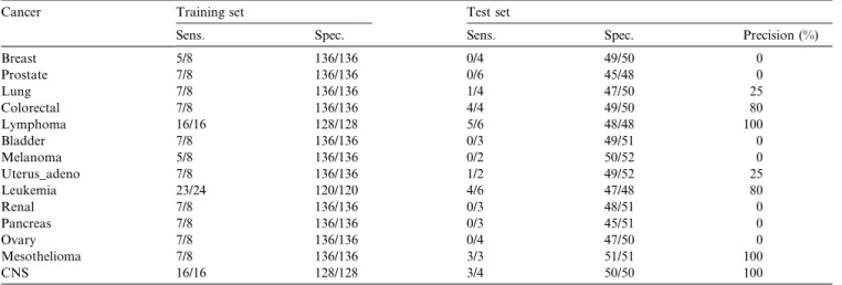
SD algorithm was used for all classes with the general-ization parametergequal to 5.Table 5presents the sen-sitivity and the specificity results for the training set and the available independent test set. Additionally, the measured precision value is computed for the test set.

FromTable 5, an interesting and important

relation-ship between prediction results on the test set and the number of target class examples in the training set can be noticed. The obtained prediction quality on the test set is very low for many classes, significantly lower than those reported in[45]. For 7 out of 14 classes the mea-sured precision is 0%. However, there are very large dif-ferences among the results for various classes (diseases). It can be noticed that the precision on the test set higher than 50% has been obtained for only 5 out of 14 classes. There are only three classes (lymphoma, leukemia, and CNS) with more than eight training samples and for all of them the induced rules have high precision on the test set, while for only 2 out of 11 classes with eight training cases (colorectal and mesothelioma) a high pre-cision has been achieved. The classification properties corresponding to classes with 16 and 24 target class examples are comparable to the performances reported for these classes in[45], yet achieved by predictors much simpler than in the mentioned work. Consequently, we select those for expert interpretation in Section 4.2.

The results indicate that there is a certain threshold on the number of available training examples below which the subgroup discovery algorithm SD is not appropriate because it can not prevent overfitting de-spite the techniques designed for this purpose.6 How-ever, it seems that for only slightly larger training sets Table 3

Rules induced for the leukemia domain for classes acute myeloid leukemia (AML) and acute lymphoblastic leukemia (ALL) Models for the AML/ALL leukemia domain

AML class‹

(LEPR_leptin_receptor EXPRESSED) AND (glutathione_s_transferase_microsomal EXPRESSED) ALL class‹

(DF_D_component_of_complement_(adipsin) NOT EXPRESSED) AND (liver_mRNA_interferon_gamma_inducing_factor NOT EXPRESSED)

To improve the interpretability of induced models, gene valuesPandAhave been replaced by EXPRESSED and NOT EXPRESSED, respectively.

Table 4

Sensitivity and specificity values for the leukemia training and test set, as well as for the leukemia samples from the multi class problem

Cancer Training set Test set Leukemia from multi-class domain

Sens. Spec. Sens. Spec. Precision (%) Sens. Spec. Precision (%)

AML 11/11 27/27 9/14 18/20 82 7/10 19/20 87

ALL 26/27 11/11 19/20 13/14 95 8/20 10/10 100

5

InTables 4 and 5, sensitivity and specificity values are presented as fractions with the denominators presenting the numbers of positive and negative examples on which the rule quality has been tested.

6 _{Improved results could be achieved by voting of best rules induced}

in several runs of the SD algorithm within the DMS covering algorithm; this work is out of the scope of this paper, as voting of numerous classifiers would hinder the interpretability of induced descriptions.

it can effectively detect relevant relationships. This con-clusion is very optimistic because we can expect signifi-cantly larger gene expression databases to become available in the near future.

Table 6 presents the rules for the three cancer types

with 16 and 24 training samples. Expert analysis of these rules in presented in Section 4.2. For all three diseases, a very good agreement in prediction results for the train-ing and the test set can be noticed, which indicates that no significant training data overfitting has occurred. The sensitivity values measured on the test set are between 66 and 83% while the specificity value is always excellent and equal or almost equal to 100%, for all the three rules.

3.3. Comparing classification performance to previous results

We now relate the predictive classification perfor-mance of the five selected rules (2 for the AML/ALL do-main and 3 for the multi-class dodo-main) obtained by subgroup discovery to predictors for the corresponding classes previously reported in [20,45,10]. Due to differ-ences in the presentation of predictive performance indi-cators in the mentioned literature, we convert them into a unified quantity of predictive accuracy, defined as the proportion of correctly classified testing instances

among all testing instances. Further, we observe the number of genes (attributes) employed in the individual predictors.

The results for the AML/ALL domain are summa-rized inTable 7. We now describe the way we calculated the classification accuracy. For the subgroup discovery algorithm, we have two rules, each obtained by viewing one of the classes as the target class. To assess predictive accuracy, the two rules can be combined into a single two-class classifier, for example by a voting mechanism supplemented by a majority-class vote for instances not complying to the conditions of any of the rules. Such a

Table 6

Rules induced for the multi-class cancer domain for cancer types with 16 (lymphoma and CNS) and 24 (leukemia) target class samples Models for the multi-class cancer domain

lymphoma class‹

(CD20_receptor EXPRESSED) AND (phosphatidyl-inositol_3_kinase_regulatory_alpha_subunit NOT EXPRESSED) leukemia class‹

(KIAA0128_gene EXPRESSED) AND (prostaglandin_d2_synthase_gene NOT EXPRESSED) CNS class‹

(fetus_brain_mRNA_for_membrane_glycoprotein_M6 EXPRESSED) AND (CRMP1_collapsin_response_mediator_protein_1 EXPRESSED) Table 7

The AML/ALL domain: comparing predictive accuracy and the number of involved genes for predictors obtained by the subgroup discovery approach (SD), by support vector machine construction (SVM), and by voting of informative genes[20]

Cancer Classifier Accuracy (%) No. of genes

AML SD 79.41 2 SVM I[10] 88.24 50 Voting[20] 93.94 50 ALL SD 94.11 2 SVM II[10] 94.11 50 SVM III[10] 97.05 50

The three versions of SVM correspond to three groups of predictors with different parameterizations and different gene sets employed, as reported by[10].

Table 5

Prediction results measured for 14 cancer types in the multi-class domain

Cancer Training set Test set

Sens. Spec. Sens. Spec. Precision (%)

Breast 5/8 136/136 0/4 49/50 0 Prostate 7/8 136/136 0/6 45/48 0 Lung 7/8 136/136 1/4 47/50 25 Colorectal 7/8 136/136 4/4 49/50 80 Lymphoma 16/16 128/128 5/6 48/48 100 Bladder 7/8 136/136 0/3 49/51 0 Melanoma 5/8 136/136 0/2 50/52 0 Uterus_adeno 7/8 136/136 1/2 49/52 25 Leukemia 23/24 120/120 4/6 47/48 80 Renal 7/8 136/136 0/3 48/51 0 Pancreas 7/8 136/136 0/3 45/51 0 Ovary 7/8 136/136 0/4 47/50 0 Mesothelioma 7/8 136/136 3/3 51/51 100 CNS 16/16 128/128 3/4 50/50 100

classifier would however no longer satisfy our require-ment of simplicity. Therefore, we rather view each of the two rules as an individual binary classifier, inter-preted under the closed-world assumption. That is, if the AML rule antecedent is not satisfied, then ALL is considered as the predicted class. The inverse principle is applied for the ALL rule. Each of the two rules is thus assigned its own accuracy value.

To calculate the predictive accuracy of the voting ap-proach in[20], we consider that their predictor provided a class decision in 29 of the 34 testing cases and this deci-sion was always correct. For the five undecided cases, we consider the accuracy of the majority vote on the test set (20

34¼58:82%). The overall accuracy value is thus

calcu-lated as29

34100%þ 5

3458:82%¼93:94%.

Finally, the SVMs in[10]provides a binary decision for all testing examples, therefore the accuracy calcula-tion is straightforward using the provided counts of (in)correct classifications (Table 3 in[10]).

Two further notes have to be made on the numbers of genes (attributes) involved in the respective predictors, as quoted in Table 7. For the voting approach, Golub et al. [20] report that the number of correct decisions was maintained at 100% when reducing the number of employed genes to as low as 10. However, it is not re-ported for how many cases the reduced classifier was able to provide a decision. Therefore, we could not cal-culate the corresponding predictive accuracy value in the manner described above. For the SVMs in[10], the per-formance was also measured with the number of em-ployed genes decreasing to as low as 4, and it was shown to fall rather quickly (see Table 2 in [10]). For a 4-best-genes attribute subset, the accuracy ranged from 54 to 93%, depending on the feature ranking meth-od and the SVM parameterization. Even these rather low accuracies reported for the simplified classifiers probably overestimate the accuracies on the correspond-ing test sets. This is because they were measured by the cross-validation procedure combining the training and test sets for induction purposes and leaving only one example for testing at each validation stage. Thus, the assessed predictors were constructed from larger train-ing sets than the predictors listed inTable 7.

Table 8 compares the predictive performance of the

selected best classifiers obtained by the subgroup discov-ery approach in the multi-class cancer domain, with the SVM predictors for the corresponding classes achieved by[45](see Fig. 4 of their paper). The accuracy for each class is measured for a binary classification task where all the examples of the given class are treated as positive and all the other examples as negative. Again, we ob-serve the number of genes employed in the respective classifiers. Ramaswamy et al. [45] also investigate whether the predictive accuracy is sensitive to a decreas-ing number of available attributes (see Fig. 5 in[45]), but we cannot use these results as they are averaged over all

classes and individual class results are not reported. However, the fact that the average accuracy of SVM falls from about 74% for 10,000 genes to about 57% for 3 genes indicates that—unlike with the SD ap-proach—satisfactory accuracy can not be expected from SVM with a very small number of employed attributes.

4. Expert evaluation of induced models

This section provides an expert evaluation of the in-duced subgroup descriptions by one of the authors (J.T.), who was not involved in the rule discovery pro-cess described above. To make the text acpro-cessible to a reader without biological background, we provide a less formal explanation of certain terms. In general, albeit a simplified view, cellular processes which increase prolif-eration (cellular division) and inhibit apoptosis (cellular death) are consistent with a phenotype of cancerous cell. 4.1. The AML/ALL domain

Cancers which originate from hematopoietic (blood) cells are called leukemias and lymphomas. Acute leuke-mias can be of either lymphoid7origin (acute

lympho-cytic leukemia, ALL) or myeloid7 origin (acute

myelogenous leukemia, AML).

The best-scoring rule for the AML disease class was the following:

AML class:

(LEPR_leptin_receptor EXPRESSED) AND (glutathi-one_s_transferase_microsomal EXPRESSED)

The first condition assumes the expression of the lep-tin receptor. The obesity gene product leplep-tin regulates food intake, but it is also important in the regulation of inflammation, immunity and hematopoiesis8 [16]. The leptin receptor, a single transmembrane-spanning molecule, is a member of the cytokine9receptor super-Table 8

Multi-class cancer domain: Comparing predictive accuracy and number of involved genes for selected predictors obtained by the subgroup discovery approach (SD) and by support vector machine (SVM) construction[45]

Class Classifier Accuracy (%) No. of genes

Lymphoma SD 98.14 2 SVM[45] 100.00 16063 Leukemia SD 94.44 2 SVM[45] 98.14 16063 CNS SD 98.14 2 SVM[45] 100.00 16063 7

A subclass of white blood cells.

8

Blood forming.

9

family. It is expressed on the hematopoietic stem cells [22], and, while absent from samples of ALL, it is fre-quently expressed in primary and secondary AML [32]. Interaction of leptin with its receptor has prolifera-tive and anti-apoptotic effect on AML blasts [32]. Leptin, secreted from bone marrow adipocytes,10 stimu-lates both myeloid7 development and bone marrow angiogenesis.11Furthermore, it has been shown[24]that inhibition of the leptin receptor signaling by anti-leptin receptor antibody decreased both microvessel formation and number of AML blasts in the bone marrow.

Regarding the second condition, Glutathion-S -trans-ferases (GST) are liver cytosolic12and microsomal12

en-zymes, which metabolize toxic substances [28].

Detoxification of toxic substances (e.g., environmental mutagens and chemotherapeutic drugs used in cancer treatment) is important for both the development of malignancies and their response to treatment. Whereas the condition regards the microsomal kind of GST, most of existing literature and knowledge is concerned with the cytosolic kind. For example, it is known that cyto-solic GST are polymorphic in humans and null variants of some GST isoforms seem to increase oxidative stress on hematopoietic stem cells. This may in turn lead to a higher incidence of leukemia or chemotherapy resistant disease with poorer outcome [53,27,33].

Concerning the possible leptin–GST interaction, it is remarkable that in a study[4] of experimental hepato-toxicity with reduced cytosomal GST in a murine model, exogenous administration of leptin resulted in decreased detoxification and high levels of reactive byproducts. Again, our model assumes the elevated expression of microsomalGST and thereby does not directly parallel the mentioned study. However, it suggests that the lep-tin receptor and GST may form a combined factor rele-vant to pathophysiology of AML, and along with[4]it motivates a further investigation of the possible interac-tion of leptin with the GST family.

The best-scoring rule for the ALL disease class was the following:

ALL class:

(DF_D_component_of_complement_(adipsin) NOT

EXPRESSED) AND

(liver_mRNA_interferon_gam-ma_inducing_factor EXPRESSED)

The first condition is concerned with adipsin, also termed complement factor13D. This is an enzyme

pro-ducing the acylation14-stimulating protein (ASP), which increases triglyceride synthesis in adipocytes10 [9]. Adipsin is expressed in cell lines derived from hu-man monocytes [5], hepatocytes15 [6], astroglioma16 [7] and gastric cancer [30], but not—to our knowl-edge—in ALL. Significantly, a recent analysis of ALL and AML transcription profiling data identified adipsin as one out of three best targets for investigating the ba-sic biology of ALL/AML and their mutual distinction [10]. Our model thus confirms this basic observation of [10], but is more informative in that it specifically articulates the absence of adipsin expression assumed for the ALL class.

Interferon-gamma-inducing factor, assumed to be ex-pressed by the second condition, was discovered in 1995 [43]and later termed interleukin-18 (IL-18). IL-18 is se-creted by activated macrophages7and induces high lev-els of interferon-gamma production in T cells17[49]. The ruleÕs assumption is compatible with the previous study [52] where increased IL-18 expression has been corre-lated with ALL. The expression has been correcorre-lated also with cutaneous18natural killer lymphoma[3], cutaneous T-cell lymphoma [3], metastatic breast cancer[37], lym-phohistiocytosis19 [51], and high risk AML[57]. It has been suggested that IL-18 could lead to antitumor effects in some cancers through induction of apoptosis[42], and that IL-18 is likely involved in the autonomy of leuke-mic cells[58].

A remark should be made concerning the mutual relationship of the two genes involved in the rule. Interferon-gamma has been observed in the human astroglioma15 cell line to stimulate the expression of complement factors13 B and C2, closely related to adipsin (complement factor D) [7]. Adipsin itself, however, was refractory to the IL-18 stimulation. This is in agreement with the simultaneous presence of IL-18 and absence of adipsin as stipulated by the rule.

4.2. The multi-class cancer domain

Here we discuss the discovered rules for three respec-tive cancer classes: lymphoma, leukemia, and central nervous system (CNS) cancers. As we have mentioned already, leukemias and lymphomas are cancers originat-ing from hematopoietic (blood) cells.

10 _{‘‘Fat cells’’.} 11 _{Forming of vessels.}

12 _{The adjectives cytosolic and microsomal refer to two different}

locations within the cell.

13

Substance present in blood that plays role in blood-clotting and immune response.

14_{Addition of a carbohydrate group.} 15_{Liver cells.}

16_{Brain cancer.}

17_{Thymus-derived white blood cell. The thymus is a gland}

respon-sible for maturation of some immune cells.

18

Skin-related.

19

Disease associated with high numbers of histiocytes (macrophages).

The following rule was found for the lymphoma class:

Lymphoma class:

(CD20_receptor EXPRESSED) AND

(phospha-tidylinositol_3_kinase_regulatory_alpha_subunit NOT EXPRESSED)

The first condition stipulates the expression of the CD20 receptor. CD20 receptor, a calcium channel,20 is a lineage-specific21B-cell22antigen present on lymphoid cells. CD20 lymphoid marker is used routinely in diag-nosis of lymphomas. The identification of this gene is thus reassuring and confirms that our search strategy is able to detect genes already known to be characteristic of specific malignancy such as lymphoma.

Phosphatidyl-inositol-3-kinase (PI3K), assumed not expressed by the second condition, is a key molecule in intracellular signaling. It transmits signals from the cel-lular membrane to the nucleus, and its activation leads to cytokine9production and cell division. PI3K is also critical for killing (cytotoxicity) of tumor cells by T cells17and natural killer (NK) cells7[59]. Therefore the absence of PI3K activation may compromise immune surveillance and result in environment permissive for malignant growth. While PI3K is a necessary for sur-vival of some leukemic cells[55,1], it is conceivable that in other malignancies, presumably driven by different proliferation signals, the absence of PI3K (with or with-out dysregulation of T cell and NK surveillance) could result in clonal proliferation and lymphoma[48,59].

For the leukemia class, we have the following rule:

Leukemia class:

(KIAA0128_gene EXPRESSED) AND (prostaglan-din_d2_synthase_gene NOT EXPRESSED)

KIAA0128 gene (Septin 6), addressed by the first con-dition, is a member of a family of filament-forming23 pro-teins, septins, forming heteropolymer complexes involved in cytoskeletal organization and cell division. Septin 6 has been identified as a fusion partner of the MLL gene in in-fants with acute leukemias[8,44,47,17]. The MLL gene is frequently rearranged and fused to partner genes in ALL and AML. Out of more than 40 gene fusion partners of MLL gene identified to-date, three are septins, and the AML type with the Septin 6 (KIAA0128 gene)—MLL fu-sion likely represents a subset on infant AML with com-mon leukemogenesis pathway[29].

The second condition is concerned with the absence prostaglandin D synthase (PGDS) expression. PGDS is an enzyme active in the production of prostaglandins (pro-inflammatory an anti-inflammatory molecules). Elevated expression of PGDS has been found in brain tumors, ovarian and breast cancer [50,26], while hema-topoietic PGDS has not been, to our knowledge, associ-ated with leukemias.

Viewing the rule as a whole, the absence of PGDS expression may be a part of the ‘‘molecular signature’’ reflecting either the general tissue type (leukocytes) or the specific, KIAA0128 (Septin 6) dependent, leukemic process. Future studies should determine whether the identification of Septin 6 is due to frequent Septin 6— MLL rearrangements in our series or whether the Septin 6 expression is associated with other types of leukemia as well. Collectively, these observations could lead to a more general role for Septin 6 in leukemias with and without MLL rearrangements.

Lastly, we address the rule found for the CNS class.

CNS class:

(fetus_brain_mRNA_for_membrane_glycoprotein_M6 EXPRESSED) AND (CRMP1_collapsin_response_me-diator_protein_1 EXPRESSED)

Concerning the first condition, the membrane glyco-protein M6 functions as a neuron-specific24 calcium channel. Upon nerve growth factor stimulation the M6 protein appears to promote neuronal differentiation [41], and the antibodies against M6 affect the survival of cerebellar25neurons[56].

As for the second condition, members of the collap-sin/semaphorin family,26 including collapsin response mediator protein 1, CRMP1, play an important role in proliferation,27 and pathfinding of growing axons to reach their targets in nervous system [12,13]. Both M6 and CRMP1 appear to have multifunctional roles in shaping neuronal networks, and their function as sur-vival (M6) and proliferation (CRMP1) signals may be relevant to growth promotion and malignancy.

5. Conclusions

This study aimed to test the feasibility of inducing simple, rule-based models for gene expression data. We argue that a major advantage of such models is their direct interpretability by domain experts. The prediction results obtained on independent test sets as well expert 20 _{A molecule on the surface of a cell membrane that facilitates the}

inflow and outflow of calcium.

21 _{Specific for a particular development path from a stem cell to a}

differentiated (specialized) cell.

22

Bone marrow (B) derived white blood cell.

23

Forming a cellular ‘‘skeleton.’’

24_{That is, it only operates in nerve cells.} 25

A specific area of the brain.

26

A family of proteins regulating the growth of neurons.

27

analysis of induced rules demonstrate that the chosen approach, based on the presented subgroup discovery methodology, can be a useful tool for the detection of relevant relationships between sample classes (diseases) and measured gene expression values. In contrast to other machine learning applications for gene expression data analysis, we have started from presence call (cate-gorical) values. Features based on presence call values are very easy for human interpretation and this signifi-cantly contributes to rules being accepted as comprehen-sible disease models.

The interpretation of the subgroup discovery results yields several biological observations: out of the five best-scoring rules (for five respective problems) selected for expert evaluation, two (lymphoma and leukemia clas-ses) are judged as reassuring and three (AML, ALL, and CNS classes) have a plausible, albeit partially speculative explanation. Namely, the best-scoring rule for the lym-phoma class in the multi-class cancer recognition prob-lem (containing 16,063 attributes) contains a feature corresponding to a gene routinely used as a marker in diagnosis of lymphomas (CD20), while the other part of the conjunction (the PI3K gene) seems to be a plausi-ble biological co-factor. The best-scoring rule for the leu-kemia class contains a gene whose relation to the disease is directly explicable (Septin 6). In the problem of distin-guishing AML from ALL, the best-scoring rule related to the AML class connects in a logical conjunction two genes, GST and leptin (out of 7192 original genes), whose co-activity was previously under biological inves-tigation in a model of impaired detoxification, and sup-ports a possibility that they may form a combined factor relevant to the etiology of AML.

In spite of the number of findings in agreement with the bio-medical state-of-the-art, discovery of known factors in the considered malignancies was not the ulti-mate goal of this study. The main goal of the method-ology is the discovery of unknown and never thought-off relationships, in a form instantly understandable to an expert. Such relationships can in turn be tested and potentially validated by means of current rapidly advancing bio-medical research and, later, clinical trials.

Although the subgroup discovery approach empha-sizes a strong restriction of the hypothesis space with the intention to prevent data overfitting, the results dem-onstrate that this phenomenon, linked to the overwhelm-ing number of existoverwhelm-ing feature combinations in the attribute-rich domain, can not be completely eliminated, especially in domains and target classes with a small number of samples. Therefore, for several target classes (with fewer than 16 positive examples) we have not been able to induce a well-generalizing rule submittable to expert interpretation. It is promising, however, that the obtained prediction quality of the induced rules grows very rapidly with the increased size of the training set

and we expect to have significantly larger gene expression domains in the near future from which it will be possible to induce comprehensible, highly reliable, and highly predictive disease models. This will help in disease pre-diction and classification, and in attempts to better understand the biology of malignancy, to risk stratify cancer patients and, in future applications, to implement treatment strategies targeted at individual patients.

Acknowledgments

This work was supported by the Croatian Ministry of Science, Education and Sport, the Slovenian Ministry of Education, Science and Sport, and the Czech Ministry of Education through the project MSM 212300013.

References

[1] Abbott RT, Tripp S, Perkins SL, Elenitoba-Johnson KS, Lim MS. Analysis of the PI-3-kinase-PTEN-AKT pathway in human lymphoma and leukemia using a cell line microarray. Mod Pathol 2003;16(6):607–12.

[2] Agrawal R, Imielinski T, Shrikant R. Mining association rules between sets of items in large databases. In: Proceedings of the ACM SIGMOD conference on management of data, Washing-ton, DC; 1993. p. 207–16.

[3] Amo Y, Ohta Y, Hamada Y, Katsuoka K. Serum levels of interleukin-18 are increased in patients with cutaneous T-cell lymphoma and cutaneous natural killer-cell lymphoma. Br J Dermatol 2001;145(4):674–6.

[4] Balasubramaniyan V, Kalaivani SJ, Nalini N. Role of leptin on alcohol-induced oxidative stress in Swiss mice. Pharmacol Res 2003;47(3):211–6.

[5] Barnum SR, Volanakis JE. In vitro biosynthesis of complement protein D by U937 cells. J Immunol 1985;134(3):1799–803. [6] Barnum SR, Volanakis JE. Biosynthesis of complement protein D

by HepG2 cells: a comparison of D produced by HepG2 cells, U937 cells and blood monocytes. Eur J Immunol 1985;15(11):1148–51.

[7] Barnum SR, Ishii Y, Agrawal A, Volanakis JE. Production and interferon-gamma-mediated regulation of complement compo-nent C2 and factors B and D by the astroglioma cell line U105-MG. Biochem J 1992;287(Pt 2):595–601.

[8] Borkhardt A, Teigler-Schlegel A, Fuchs U, Keller C, Konig M, Harbott J, et al. An ins(X;11)(q24;q23) fuses the MLL and the Septin 6/KIAA0128 gene in an infant with AML-M2. Genes Chromos Cancer 2001;32(1):82–8.

[9] Cianflone K, Xia Z, Chen LY. Critical review of acylation-stimulating protein physiology in humans and rodents. Biochim Biophys Acta 2003;1609(2):127–43.

[10] Chow ML, Moler EJ, Mian IS. Identifying marker genes in transcription profiling data using a mixture of feature relevance experts. Physiol Genom 2001;3(5):99–111.

[11] Clark P, Niblett T. The CN2 induction algorithm. Machine Learn 1989;3(4):261–83.

[12] Cohen-Salmon M, Crozet F, Rebillard G, Petit C. Cloning and characterization of the mouse collapsin response mediator protein-1, Crmp1. Mamm Genome 1997;8(5):349–51.

[13] Deo RC, Schmidt EF, Elhabazi A, Togashi H, Burley SK, Strittmatter SM. Structural bases for CRMP function in plexin-dependent semaphorin3A signaling. EMBO J 2004;23:9–22.