© 2012 INFORMS
The Joint Sales Impact of Frequency Reward and
Customer Tier Components of Loyalty Programs
Praveen K. Kopalle
Tuck School of Business at Dartmouth, Dartmouth College, Hanover, New Hampshire 03755, [email protected]
Yacheng Sun
Leeds School of Business, University of Colorado, Boulder, Colorado 80309, [email protected]
Scott A. Neslin
Tuck School of Business at Dartmouth, Dartmouth College, Hanover, New Hampshire 03755, [email protected]
Baohong Sun
Cheung Kong Graduate School of Business, New York, New York 10019, [email protected]
Vanitha Swaminathan
Katz School of Business, University of Pittsburgh, Pittsburgh, Pennsylvania 15260, [email protected]
W
e estimate the joint impact of the frequency reward and customer tier components of a loyalty program oncustomer behavior and resultant sales. We provide an integrated analysis of a loyalty program incorpo-rating customers’ purchase and cash-in decisions, points pressure and rewarded behavior effects, heterogeneity, and forward-looking behavior. We focus on four key research questions: (1) How important is it to combine both components in one model? (2) Does points pressure exist in the context of a two-component loyalty program? (3) How is the market segmented in its response to the combined program? (4) Do the programs complement each other in terms of the incremental sales they produce?
Our most basic message is that the frequency reward and customer tier components of loyalty programs should be modeled jointly rather than in separate models. We find strong evidence for points pressure for both the customer tier and frequency reward components using both model-based and model-free evidence. We find a two-segment solution revealing a “service-oriented” segment that highly values cash-ins for room upgrades and staying in “luxury” hotels, and a “price-oriented” segment that is more price sensitive and highly values the frequency reward aspects of the loyalty program. Furthermore, we find that both components generate incremental sales. Also, there was slight synergy between the programs but not a huge amount. Overall, each component contributes to increased revenues and does not interfere with the other.
Key words: loyalty program; customer tier programs; frequency reward; database marketing; segmentation
History: Received: June 1, 2009; accepted: September 1, 2011; Eric Bradlow and then Preyas Desai served as
the editor-in-chief and K. Sudhir served as associate editor for this article. Published online inArticles in
AdvanceJanuary 24, 2012.
1. Introduction
Loyalty programs, designed to maintain and enhance loyalty, have become “go-to” marketing programs for many companies (Deighton 2000, Lewis 2004, Liu 2007, Zeithaml et al. 2001). In recent years, vari-ous firms have initiated loyalty programs and have supported these programs with investments in cre-ating and maintaining databases on loyalty program members. For instance, a recent survey conducted by research companies Ipsos Mori/The Logic Group suggests that almost two thirds (62%) of people say they belong to at least one loyalty program,
although only 26% agree that it leads to greater loy-alty (Barnett 2010).
Thus, despite the growth of loyalty programs, their value to the firm is a source of debate. Advocates view loyalty programs as a means to soften price competition (e.g., Kim et al. 2001, Klemperer 1987) or build a customer database (Butscher 1998, Reynolds 1995), and as a dominant strategy when fixed costs are low (Kumar and Rao 2006). Because a minority of customers often contribute most to a firm’s prof-its, it is logical to lavish attention on them (Peppers and Rogers 1997). Critics, however, cite high program costs (Dowling and Uncles 1997), question whether 216
Thi
s
file
is
p
ro
vide
d
fo
r
in
formationa
l
purpose
s
on
ly
an
d
m
ay
no
t
b
e
re
distributed.
they really increase loyalty (Keiningham et al. 2006, Hartmann and Viard 2008, Sharp and Sharp 1997, Shugan 2005), and see them as a potential prisoner’s dilemma (Kopalle and Neslin 2003).
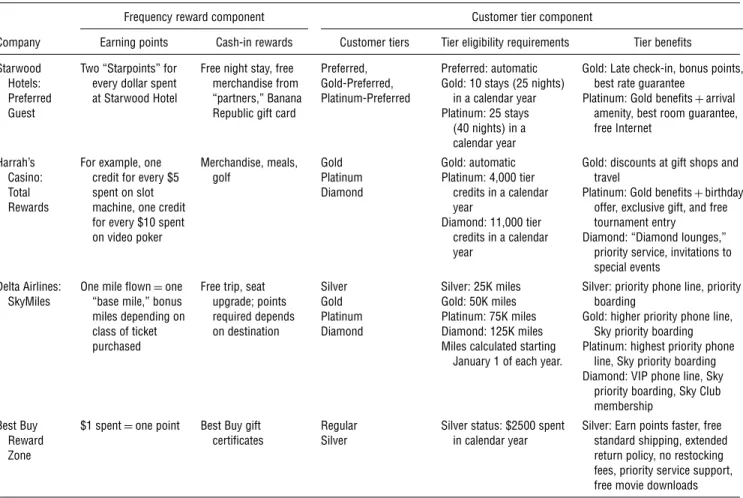
One factor muddling this debate is that loyalty pro-grams consist of two distinct components: frequency reward and customer tier (Blattberg et al. 2008). Dif-ferentiating the relative effectiveness of these two components is important for evaluating and diagnos-ing the impact of any loyalty program. Frequency reward programs are of the form “buy X times, get something free.” These are the original trading-stamp programs. Customer tier programs are of the form “once you qualify for our diamond tier, we will pro-vide you with special benefits and services.” Table 1 provides brief examples of loyalty programs, where we clearly see the frequency reward and customer tier components.
Both loyalty program components rely on accumu-lated customer sales to determine which customers qualify for which rewards. However, they differ in the nature of the reward as well as the means by which
Table 1 Examples of Loyalty Programs Showing Frequency Reward and Customer Tier Components
Frequency reward component Customer tier component
Company Earning points Cash-in rewards Customer tiers Tier eligibility requirements Tier benefits
Starwood Hotels: Preferred Guest
Two “Starpoints” for every dollar spent at Starwood Hotel
Free night stay, free merchandise from “partners,” Banana Republic gift card
Preferred, Gold-Preferred, Platinum-Preferred
Preferred: automatic Gold: 10 stays (25 nights)
in a calendar year Platinum: 25 stays
(40 nights) in a calendar year
Gold: Late check-in, bonus points, best rate guarantee
Platinum: Gold benefits+arrival amenity, best room guarantee, free Internet
Harrah’s Casino: Total Rewards
For example, one credit for every $5 spent on slot machine, one credit for every $10 spent on video poker
Merchandise, meals,
golf GoldPlatinum
Diamond Gold: automatic Platinum: 4,000 tier credits in a calendar year Diamond: 11,000 tier credits in a calendar year
Gold: discounts at gift shops and travel
Platinum: Gold benefits+birthday offer, exclusive gift, and free tournament entry
Diamond: “Diamond lounges,” priority service, invitations to special events
Delta Airlines:
SkyMiles One mile flown“base mile,” bonus=one miles depending on class of ticket purchased
Free trip, seat upgrade; points required depends on destination Silver Gold Platinum Diamond Silver: 25K miles Gold: 50K miles Platinum: 75K miles Diamond: 125K miles Miles calculated starting
January 1 of each year.
Silver: priority phone line, priority boarding
Gold: higher priority phone line, Sky priority boarding Platinum: highest priority phone
line, Sky priority boarding Diamond: VIP phone line, Sky
priority boarding, Sky Club membership
Best Buy Reward Zone
$1 spent=one point Best Buy gift
certificates RegularSilver Silver status: $2500 spentin calendar year Silver: Earn points faster, freestandard shipping, extended return policy, no restocking fees, priority service support, free movie downloads Sources.See the following for complete descriptions (all accessed September 22, 2010): Starwood Hotels: http://www.starwoodhotels.com/preferredguest/ account/member_benefits/index.html, Harrah’s Casino: http://www.harrahs.com/total/_rewards/overview/overview.jsp, Delta Skymiles: http://www.delta.com/ skymiles/index.jsp, and Best Buy Reward Zone: https://myrewardzone.bestbuy.com/.
Note. The descriptions present summaries and examples.
customers attain it. First, a frequency reward is a one-shot affair—the customer redeems points for a free stay at a hotel, a free flight, a coupon, etc. In contrast, customer tier programs offer a steady stream of ben-efits as long as the customer is a member of that tier. Second, frequency reward programs typically require customers to proactively redeem their points, and cus-tomer tier programs dispense their reward automat-ically. Once customers qualify for a certain tier, they are notified and treated according to their tier status. Third, there is usually no expiration date for points inventory accumulated under frequency reward pro-grams; in contrast, customer tier status does expire and needs to be re-earned.
Prior loyalty program research (e.g., Lewis 2004) has focused on the frequency reward component. This work (e.g., Bolton et al. 2000, Lal and Bell 2003, Roehm et al. 2002, Taylor and Neslin 2005) provides evidence of rewarded behavior effects; i.e., a reward earned in the last period increases the likelihood of repatronage in the next period. In a laboratory set-ting, Kivetz et al. (2006) and Nunes and Drèze (2006)
Thi
s
file
is
p
ro
vide
d
fo
r
in
formationa
l
purpose
s
on
ly
an
d
m
ay
no
t
b
e
re
distributed.
have demonstrated the points pressure effect; i.e., cus-tomers increase their purchase frequency as they get closer to earning a frequency reward. Akin to Lewis (2004), we demonstrate the effect using actual pur-chase data. In addition, however, we investigate the extent to which points pressure effects exist sepa-rately for a customer tier program and for a frequency reward program.
With the exception of Drèze and Nunes (2008), very little has been learned about customer response to customer tier programs, particularly in a dynamic set-ting (see Blattberg et al. 2008). To our best knowledge, prior research has not studied frequency reward and customer tier programs in an integrated way. This does not sit well with the fact that many compa-nies offer customer tier programs alongside the fre-quency reward component, as illustrated in Table 1. The key point is that in practice, both tier and fre-quency components are common elements of loyalty programs. As a result, an evaluation of a loyalty pro-gram requires an integrated analysis of both com-ponents. The purpose of this paper is to develop and estimate a model to provide such an evaluation, which allows us to answer the following questions:
• How important in terms of insight and model fit is it to combine the tier and frequency components in one integrated model?
• Do “points pressure” effects exist for both com-ponents? For example, do customers increase their purchase rate as they approach higher tier status?
• How is the market segmented in terms of response to the loyalty program? Is there a “frequency reward” segment and a “customer tier” segment?
• Are the frequency and tier components comple-mentary in terms of incremental sales produced by the program?
To address these issues, the model must contain the following phenomena.
(a) Forward-Looking Customers—Both frequency re-ward (e.g., free hotel stay) and customer tier benefit (e.g., elite status) components encourage customers to consider the future ramifications of their current choices, because these choices bring them closer to receiving a reward.
(b) Obtaining the Reward—For the frequency reward program, this requires an endogenous decision to “cash in.” In contrast, customer tier reward is deliv-ered automatically.
(c) Customer Heterogeneity—This addresses the issue of market segmentation.
(d) Rewarded Behavior—The reward indeed is short term, but customer affect created by the reward can translate into an increase in loyalty.
We apply our model to the loyalty program insti-tuted by a major hotel chain. The analyses yield interesting results: (1) Including frequency reward
and customer tier components in the same model improves model fit and yields additional insights. (2) There is a significant points pressure effect for both components. (3) There are rich customer seg-ments where customers vary in their responses to the frequency and customer tier components as well as to price. (4) Both components produce incremental sales, with some complementarity but no cannibaliza-tion between the two components.
In summary, the contribution of this paper is threefold. First, we provide an integrated analysis of the impact of two important components (fre-quency reward and customer tier) of a loyalty pro-gram on customer behavior and corresponding sales. Second, we endogenize the cash-in decision for the frequency reward, a factor not considered in previ-ous work. Third, we add to the empirical knowledge base on how loyalty programs work in terms of points pressure, rewarded behavior, and incremental sales impact.
One novel aspect of our paper relative to previous work is the inclusion of explicit measures of compet-itive activity (competcompet-itive price and occupancy rates). We indeed find that competitive activity has a neg-ative impact on sales, although that impact differs by market segment. Although this is an advance and shows the desirability of including competitive mea-sures, our results must be seen as exploratory because we cannot differentiate competitive hotel stays from no stays, and our policy implications do not imply an equilibrium analysis that allows for competitive response. We will discuss this issue in more detail when we report competitive effects and policy simu-lations. But first we discuss the model, the data, and then the empirical results.
2. Model
2.1. BackgroundThe model is generally applicable to loyalty pro-grams comprising both frequency reward and cus-tomer tier components. To make the exposition clear, we describe the model in the context of our applica-tion to a hotel’s loyalty program. The hotel catego-rizes each of its properties as “economy,” “regular,” or “luxury.” All properties allow customers to cash in points for a free night, whereas cash-in for a room upgrade is only available at a luxury property. Points are accrued via paid stays, they do not expire, and no points are earned on free stays. Customers need to contact the hotel if they wish to cash in points. Customers could not cash in for two rewards at once, e.g., a free stay at a luxury hotel plus an upgrade. The tier component places customers in the Base, Platinum, or Diamond tier depending on how many
Thi
s
file
is
p
ro
vide
d
fo
r
in
formationa
l
purpose
s
on
ly
an
d
m
ay
no
t
b
e
re
distributed.
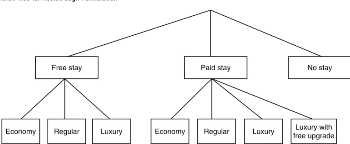
Figure 1 Decision Tree for Nested Logit Formulation
Economy Regular Luxury Economy Regular Luxury free upgradeLuxury with
Free stay Paid stay No stay
paid stays they had during the past calendar year.1
Tier benefits include better service, priority check-in, lounge access, service recovery assistance, etc. Upon reaching a tier threshold during a calendar year, cus-tomers are informed of their status and provided with the service level commensurate with their tier for the rest of that calendar year as well as the following year.
2.2. Customer Decisions
In formulating the model, we recognize that the cus-tomer faces two fundamental decisions—the “stay” decision and the “accommodation” decision. The stay decision is whether to stay at the hotel paying full price, paying no price (a free stay), or not staying at all. The accommodation decision entails the specific level of hotel—regular, economy, luxury, or upgraded room in a luxury hotel. We therefore will formulate a nested logit model, with the decisions organized as in Figure 1.
In addition to capturing the two types of decisions (stay versus accommodation), organizing the choices this way accounts for unobserved factors that system-atically elevate some stay decisions over others. For example, a business trip will increase the utility of paid stay because a third party may be paying for the trip. The nested logit model will then capture the ele-vation of utilities for all four accommodation choices within paid stay. A leisure trip will increase the utility of a free stay, and similarly, the three choices within free stay. We now describe this formulation in detail. We consider i = 1� � � � � I customers who make choices at time t. Define Cimt to indicate which choice the customer makes regarding the stay deci-sion. Specifically,Cimt=1 if customer ichooses alter-nativemat timetand 0 otherwise, where
m= 0→no stay� 1→paid stay� 2→free stay� (1a)
1Note from Table 1, this reliance on “calendar year” purchases to
assign tiers appears to be common.
We define Dint to indicate which choice the customer makes regarding the accommodation decision. Specif-ically, Dint =1 if customer i chooses alternative n at timetand 0 otherwise, where
n= 1→economy� 2→regular� 3→luxury�
4→luxury with free upgrade�
(1b)
2.3. Customer Utility
We define Uimnt as the customer i’s utility for the choice combination (m� n) at time period t, which is part of an underlying dynamic model discussed in the next section, and where the allowable combina-tions of mand n are defined by the nested logit tree above. Then
Uimnt=UC
imt+UintD +�imt+�imnt� (2) where
UC
imt=utility determining choice among no stay, stay, and paid stay, because of factors observed by the researchers;
UD
int=utility determining choice among economy, regular, luxury, and luxury with free upgrade accommodations, because of factors observed by the researcher;
�imt=contribution to utility because of unobserved factors determining choice among no stay, stay, and paid stay; and
�imnt=contribution to utility because of unobserved factors determining choice among all possible choice combinations (m� n).
A key term in this formulation is the unobserved random effect �imt. After controlling for competitor price and occupancy rates, leisure travel might sys-tematically tilt utility toward free stay. This would result in a relatively large value of�i2t. All accommo-dation types under free stay would share a boost in
Thi
s
file
is
p
ro
vide
d
fo
r
in
formationa
l
purpose
s
on
ly
an
d
m
ay
no
t
b
e
re
distributed.
utility. On the other hand, business travel might sys-tematically tilt utility toward paid stay (�i1t would be large) and boost utility for all accommodation types under paid stay. Using this formulation, we therefore can account for a factor we are unable to observe— business or leisure travel.
The last term in Equation (2),�imnt, represents unob-served time-specific determinants of customeri’s util-ity for choice combination (m� n). We assume the �imnts are independent, identically distributed extreme value random variables. This treatment is consistent with prior research (Ben-Akiva and Lerman 1985, Chib et al. 2004, Chintagunta 2002, Erdem et al. 2003, Sun 2005).
We will now specify the model for observed factors affecting type of stay (no stay, paid stay, free stay):
UC imt= �i0PCt+�i1ORt form=0� �i2BHUi+�i3WDSi+�i1Ci2t−1 +�i2 2 � d=1 Cidt−1+�2 s=1 �isEist form=1�2� (3)
The outside option (m=0) corresponds to either (1) the customer does not stay at any hotel at all or (2) the customer stays at a competitive hotel. Unfor-tunately, we do not have the data to distinguish between these possibilities. This is similar to the sit-uation faced by previous researchers, e.g., Gönül and Srinivasan (1996) and Lewis (2004). Nevertheless, we can address this to some extent by having the util-ity of not staying in the hotel depend on competitive prices (PCt) and competitor occupation rate (ORt, the number of rooms sold divided by number of rooms available). Thus, �i0 and �i1 can be interpreted as
the extent to which change in competitors’ price and vacancy affects the relative attractiveness of staying with the focal hotel. We expect both �i0 and �i1 to
be negative because high prices and occupancy rates make competitors unattractive.
The utility of staying in the hotel, be it a free or paid stay, is influenced by five observed factors: (1) Base hotel usage rate measured by the number of stays in the initialization period (BHUi�.2 We expect �i2>0.
(2) The customer’s propensity to stay on weekdays versus weekends, measured by the number of stays that start on a weekday in the initialization period (WDSi�. The sign of �i3 could be positive or
neg-ative, depending on whether weekday stayers are more likely to visit the hotel (�i3>0) or less likely
(�i3<0). A positive�i3thus suggests the hotel is more
2The first 52 weeks of the data are used for initialization. We believe
this is long enough to smooth out the variations in factors such as price promotion and seasonality. Previous research (e.g., Bucklin et al. 1998) also used a similar length for the initialization period.
geared toward business travelers, because they are more likely to have a large number of weekday stays in the initialization period (a negative�i3would
sug-gest non-weekday stayers; e.g., leisure travelers are the more likely hotel visitors).3 (3) �
i1 represents the
strength of rewarded behavior, i.e., the impact on util-ity in period t if the customer received a free stay in the previous period (Ci2t−1=1). Based on previous
research, we expect�i1>0 because receiving a reward increases customer “delight” (Rust and Oliver 2000) and therefore increases subsequent utility.4(4)�
i2
cap-tures state dependence, i.e., the impact on utility in period t if the customer stayed in the focal hotel in the previous period (Ci1t−1=1 or Ci2t−1=1). As in
most previous choice model research, we expect the state dependence effect to be positive (�i2>0). (5)�is denotes the utilities of membership in customer tiers (Ei1t=1 if the customer is in the Platinum tier and 0 otherwise;Ei2t=1 if customer is in the Diamond tier and 0 otherwise). Because tier membership provides extra benefits and the Diamond tier provides the most benefits, we expect �i2> �i1>0.
Note that price of the focal hotel does not appear in the above formulation. Price will be included in the various accommodation types and impact the choice of paid versus free versus no stay via the inclu-sive value in the nested choice probabilities (Equa-tion (15)). We now specify the utility models that determine choice among accommodation types:
UintD = 0 form=0� �in+�i4Pnt form=1� n=1�2�3� �i0+�i3+�i4P3t form=1� n=4� �i1+�in form=2� n=1�2�3� (4)
For no stay (m=0), there is no accommodation decision, and we set utility equal to zero for scal-ing purposes. For a paid stay (m= 1), we define alternative-specific constants � for economy (n=1), regular (n=2), and luxury (n=3), and we expect �i3> �i2> �i1. We express the alternative-specific
util-ity for the luxury upgrade (n=4) as�i3(staying in the luxury hotel) plus �i0, which captures the additional utility as a result of the upgrade. We expect �i0>0. Note also that price for economy, regular, or luxury
3As a simplification, we assume the�s do not differ by the stay
branches of the nested logit tree. This means that, e.g., the impact of base hotel usage rate is the same on the utility of both paid and free stays. However, this does not mean these two utilities are equal. First, the unobserved factor�imt will cause them to differ, and the inclusive value term from the lower part of the nest will cause these utilities to differ.
4Note, however, an alternative possibility is that�
i1would be
neg-ative because of purchase acceleration; that is, customers move for-ward purchases in time and therefore purchase at a lower rate after they cash in, i.e., a “post-promotion dip” (Neslin 2002, pp. 23–24).
Thi
s
file
is
p
ro
vide
d
fo
r
in
formationa
l
purpose
s
on
ly
an
d
m
ay
no
t
b
e
re
distributed.
hotels now enter the utility function (Pnt). For a free stay (m=2), we need not include price because the price is zero. However, we have the same alternative-specific constants for each hotel type, plus a term (�i1)
indicating utility for a free stay.5 Intuition suggests
�i1>0 because of the “transaction utility” of a great “deal” (Thaler 1985). However, if the hassle costs are high for cashing in points, it is possible that�i1<0.
2.4. Points Accumulation
We now introduce notation to represent the points requirements of the frequency reward and customer tier requirements. DenoteR1 as the points inventory requirement for an upgrade, and let R2, R3, and R4 denote the points requirements for a free stay at econ-omy, regular, and luxury properties, respectively. Let Tsdenote the required number of paid stays for tiers. The structure of a two-component loyalty program in our case can thus be summarized by the vector (R1� R2� R3� R4� T1� T2).
Customers must accrue enough points to choose either an upgrade or a free stay. Points “inventory” accrues as follows:
INVit+1=INVit+PointsAccruedit
−PointsCashedInit� (5) where
INVit+1= customeri’s cumulative points inventory
at the beginning of periodt+1,
PointsAccruedit= points earned by customer i in periodt,6and
PointsCashedInit= points cashed in for either an upgrade or a free stay by customeriint.
Notice that the points inventory determines the choice set of the customer. Not staying in the hotel and a paid stay are always options for the customer. If customerihas enough points for an upgrade, then the choice set would include (m=1, n=4). If she is eligible for a free stay in an economy hotel, then (m= 2, n =1) is included in the choice set, etc. In essence, we have an economic model of consumer choice under cutoffs (see Swait 2001 for a detailed dis-cussion).
At the beginning of each calendar year, the inven-tory of paid stays (INVP) is reset to zero and accrues during the year according to the following equation:
INVPit+1=INVPit+PStayit� (6)
5Note that theincrementalutility of a free stay relative to a paid
stay at propertynfor customeriis�i1−�i4Pnt, and this increases with higher prices (�i4<0).
6The hotel we study allowed customers to purchase a very limited
number of points. However, we find no evidence of this in our data, perhaps because of the generally high level of points inventories carried by customers.
where
PStayit= number of paid stays added to customer i’s inventory in periodt.
Membership in a customer tier, s, is determined as follows: Eist=
1 ifTs≤min�INVPit�INVPi�LastYear� and
max�INVPit�INVPi�LastYear� < Ts+1�
0 otherwise�
(7) where
Eist= indicator variable signifying that customer i is in customer tiers at periodt,7
Ts= required number of paid stays for tiers, INVPit= number of paid stays by customer i at periodt in the current calendar year, and
INVPi�LastYear= number of paid stays by customeri
during the last calendar year.
Note our model captures the typical situation (see Table 1) that the requirements for the frequency and tier rewards are often based on different accumulation rules. First, whereasINVPitwill expire at the end of a calendar year,INVit will never expire. Second, when the customer chooses a paid stay, INVPit will always increase by one. On the other hand, the amount by which INVit increases depends on the monetary expenditure of the customer, which depends on her utilities for different hotel levels. Third, when cus-tomers make a cash-in decision, INVit will decrease, and furthermore, the exact amount of decrement depends on what reward the customer redeems for; on the other hand, INVPit will not decrease as the result of a cash-in decision.
2.5. Forward-Looking Customers
Customers must accumulate points or paid stays to qualify for a frequency reward or attain a higher cus-tomer tier. This naturally requires cuscus-tomers to be for-ward looking. For example, customers who value a high tier will consider that each stay adds to the like-lihood they will achieve this goal. The same goes for customers who value the cash-in reward. However, there is an interesting dynamic interaction between the frequency reward and customer tier components: for example, a forward-looking customer may not wish to cash in for a free stay because free stays do not count toward tier status. This decision process can be represented by a dynamic model, whereby the cus-tomer makes current period decisions that maximize her long-term utility. We express the customer’s deci-sion problem as max Cimt� Dint� m� n∈Nit E ��� t=1 � m� n∈Nit �
Uimnt·Cimt·Dint
�
�t−1�� (8)
7We know from the data what tier the customer was in initially, so
we have an initial value forEist.
Thi
s
file
is
p
ro
vide
d
fo
r
in
formationa
l
purpose
s
on
ly
an
d
m
ay
no
t
b
e
re
distributed.
where � is the per period discount factor and Nit is customer i’s choice set at time t. The operator E�·� (we suppress the subscripts i and t for expositional simplicity) is the conditional expectation given the customer’s information at time t. The value func-tion (Bellman equafunc-tion), expressing the maximum expected utility the customer can expect, given he or she is in periodt, is given by
Vit�INVit�INVPit� Fit� Cimt−1�
= max Cimt� Dint� m� n∈Nit Vimnt = max Cimt� Dint� m� n∈Nit � Uimnt+�E �
Vi� t+1�INVi� t+1�
INVPi� t+1� Fit+1� Cimt�
��
� (9) whereFitdenotes the current calendar year period for customeriindicated by periodt. This is a state vari-able because it reflects seasonality (see §2.6 for how seasonality enters the model) and the time remain-ing before customeri’s current tier status expires. The decision rule is to choose the decision�m� n�that max-imizes the choice-specific value functionVimnt:
Vimnt=Uimnt+�E�Vi�t+1�INVi�t+1�INVPi�t+1�Fit+1�Cint�
�
� (10) The state variables are as follows: inventory of total points (INVit+1�, given by Equation (5); inventory of
paid stays (INVPit+1�, given by Equation (6); and past
decision �Cint� and the calendar period (Fit+1�. Given
the complexity of the dynamic programming prob-lem, we adopt linear interpolation (Keane and Wolpin 1994) to estimate the model. See the appendix for a description of our solution approach for parameter estimation, dynamic programming algorithm, and lin-ear interpolation.
2.6. Customer Expectations of Future Demand and Prices
The customer’s decision is derived from a dynamic program. Therefore, when evaluating expected future utility, customers need to incorporate their expecta-tions regarding (1) future prices at different types of properties of the focal hotel chain, (2) price of the competitors, and (3) length of stay with the hotel. These, in turn, determine their expected future points. We assume that consumer i has rational expecta-tions for the prices of the focal company’s accommo-dation typen(Pint,n=1�2�3):
lnPint=�1in+�3
k=1
�1+k� iSkt+�int� n=1�2�3� (11)
Pint is individual specific and depends on seasonality, captured by dummy variables Skt� k=1�2�3, where �nt is the error term and
S1t=1�tis either in December, January, or February�� 0 otherwise�
S2t=1�tis either in March, April, or May�� 0 otherwise� and S3t=1�tis either in June, July, or August��
0 otherwise�
(12)
Consumers’ expectations for the competitive price and occupancy rate are modeled similarly:
lnPCit=�1ic+ 3 � k=1 �1+k� icSkt+�ict� (13.1) lnORit=�1io+�3 k=1 �1+k� ioSkt+�iot� (13.2) Thus, �1in (n=1�2�3), �2−4� i, �1ic, �2−4� ic, �1io, and �2−4� io characterize consumers’ expectations. We esti-mate these coefficients by assembling the focal price, competitive price, and occupancy rate data in a time series and then estimating each equation using ordinary least squares. We follow a two-step approach for compiling the customer-specific prices and com-petitive occupancy rates needed for these regressions. The first step is to determine the location of the city relevant to the customer; the second step is to assem-ble the prices and occupancy rates for that location (see the appendix for further details). If the customer stayed in the focal hotel in periodt, we know directly from the data the price for that accommodation and the occupancy rate (and price) of competitors in that period. If the customer did not stay in the focal hotel in period t, we still observe competitive data, and we impute prices at the focal hotel using the average price paid by other consumers for the same accom-modation during periodt in that city. This method is similar to the imputation of missing price information in packaged goods categories (e.g., Erdem et al. 2008). The averageR2(across customers) for these equations were 0.42 (Pi1t�, 0.35 (Pi2t�, 0.36�Pi3t�, 0.91 (PCit�, and 0.55 (ORct�.
Customers also have expectations regarding their length of stay, denoted LOSit, where LOSit ∼ left-truncated Normal�LOSi� �LOS2 i�. We determine the respective means �LOSi� and standard deviations ��LOS2
i� of these distributions from each customer’s transaction history during the initialization period. These distributions are then used in computing future value function, where we draw from corresponding normal distributions with the estimated means and variances (see the appendix for further details).
Thi
s
file
is
p
ro
vide
d
fo
r
in
formationa
l
purpose
s
on
ly
an
d
m
ay
no
t
b
e
re
distributed.
Note that these expectations, and the resultant choices and points accrual that emerge from them, are not explicitly included in the utility function. However, they play an important role in solving the dynamic program and hence in our predictions and estimates, because the inventory of points is a state variable (Equation (9)). Therefore, the customer max-imizes utility, taking into account the likely points accumulation scenario that will result from his or her choices.
2.7. Heterogeneity and Estimation
A long history of work in the choice models liter-ature has established the importance of incorporat-ing cross-consumer heterogeneity. Two fundamental ways of modeling heterogeneity are continuous and latent class. We adopt latent class because one of our goals is to identify and interpret segments, and latent class naturally reveals those segments (Kamakura and Russell 1989). Let�l=�jl� �1l� �2l� �0� l� � � � � �4� l� �1l� �2l� �sl,j=1�2, 3;s=1�2 be the vector of coefficients to be estimated for each latent classl. Then, the like-lihood function of the sequence of choices of all cus-tomers is L���= L � l=1 I � i=1 T � t=1 2 � m=0 4 � n=1 �
Cimt·Dint·Pr�Cimt=1�
·Dint=1�INVit�INVPit� Sit� Cim� t−1�
Din� t−1� �l� i∈l�·Pr�i∈l�
�
� (14) wherelindexes latent classes and Pr�i∈l�, the proba-bility customeriis in latent classl, is estimated. Given the extreme value distribution of the error term, the probability customeriin latent classlmakes decision �m� n�at timet is
Pr�Cimt=1�Dint=1�INVit�INVPit�Sit�Cim�t−1�Din�t−1�
�l� i∈l�=
�
eUC
imt+�m·ln�ne�UintD+�·EVimnt�
�
je UC
ijt+�j·ln��he�UihtD+�·EVijht�� � · � e�UD int+�·EVimnt� � he�U D iht+�·EVimht� � � (15) where UC
imt and UintD are defined in Equations (3)
and (4), respectively; � is the discount factor; EVimnt is the integrated value function on the pair ��imt+1� �imnt+1�; and ln��he�U
D
int+�·EVimnt��is the inclusive
value for alternative m. This inclusive value is 0 for m=0. Finally,�j,j=1�2 are the log-sum coefficients. The estimation (see the appendix) is performed using one year of data (26 biweekly periods), assum-ing a finite, forward-lookassum-ing horizon that goes one year beyond the end of the data (total of two years). In an earlier version of the model, when we did not use initialization variables, we utilized 52 biweeks
for our estimation, and the results regarding tier and reward response were quite similar to the results we obtain now with 26 biweekly periods. We use cus-tomer biweek as the unit of analysis because that period is long enough to cover the full length of all stays yet short enough so there are no multiple stays within a period. We use a finite horizon for the fol-lowing reasons.
1. This is an approximation that is computation-ally attractive relative to the infinite horizon problem. What is important in the context of our interpolation is that the parameters of the regression interpolation should stabilize before the last data period is reached (Erdem et al. 2008); indeed, they do stabilize in our estimation. Furthermore, in our algorithm, the value function calculation is for a total of two years; i.e., cus-tomers are looking ahead one year beyond the last period of our data. Allowing customers to look ahead an additional year outside of data not only approx-imates an infinite horizon problem but also ensures that the last period in our data holds the same impor-tance regardless of the period a customer is in at a given point in time. This thus allows the customer to consider the benefits of reaching a certain tier in year 1 and reaping the benefits in year 2.
2. Using a finite horizon is consistent with previous dynamic structural models (e.g., Erdem and Keane 1996; Erdem et al. 2003, 2008; Sun et al. 2003; Sun 2005 in a brand choice context; and Lewis 2004 in a frequency reward program context).
3. The limitation of the finite horizon is that at the end of that horizon there is no salvage value. Our approach limits the amount of “end game” behavior on the part of the customer in the last period of the data, because the customer is considering the implica-tions for the following year. Consequently, customers are taking into consideration the additional one-year benefit of achieving higher tier status or of having a higher points inventory.
3. Data
Our data for the hotel application are from the loyalty program of a major hotel chain, covering 3,907 cus-tomers who were members of the hotel’s loyalty pro-gram8 over two years (January 1, 2002–December 31,
2003). Included are the dates of stay by customer, type of property stayed in (economy, regular, or lux-ury), price paid,9points earned, etc. Each trip includes
8This suggests that our results apply strictly to the population of
focal hotel loyalty card holders. However, (1) this is a very impor-tant group for hotel managers, (2) our sample is not unusually loyal, averaging a reasonable 3.0 stays per year, and (3) our later findings of significant competitive effects suggest that they are not single-brand loyal.
9Note that because we observe price paid but not the list price
of all accommodations, we must impute the price available for a
Thi
s
file
is
p
ro
vide
d
fo
r
in
formationa
l
purpose
s
on
ly
an
d
m
ay
no
t
b
e
re
distributed.
a code indicating whether a reward was redeemed on that trip and, if so, how many points were used. The database also provides the beginning inventory of points for each customer and his or her tier sta-tus. We integrated these data with the competitor pricing and occupancy rates, which were purchased from Smith Travel Research, a syndicated data firm that tracks pricing and occupancy information for the hotel industry on a monthly basis. These data cov-ered hotels in each of the 14 submarkets (e.g., Los Angeles Airport vicinity, San Diego–La Jolla area, San Francisco–Market Street area, San Francisco–Nob Hill/Wharf area) in which our customers exclusively stayed. The competitive pricing and occupancy data were combined with the customer stay information from the focal hotel chain based on the time variable. Our focal chain’s policy does not allow points to be accumulated from other sources, and our data include all point transactions. An analysis of our data revealed that all customer stays involved hotel points accumulation; i.e., there were no occurrences where a customer paid for a stay at the hotel and no points were awarded to her account. There were no cases where significant hotel points, unrelated to a paid stay, were added to a customer’s account. Further-more, point redemption from a customer’s account at any time was always associated with that customer staying with the chain in that period.
The hotel’s frequency reward program involves four categories of frequency reward: free stay at an economy (5,000 points), regular (8,000 points), or lux-ury (12,000 points) property, and a free upgrade at a luxury property (3,000 points). Five points are earned per dollar spent, while Platinum and Diamond tier members earn an additional 15% and 30%, respec-tively, per dollar spent.10 The requirements for
num-ber of paid stays for Platinum and Diamond tiers are 5 and 12, respectively. Customers assigned to higher tiers in a calendar year, YR (based on paid stays in year, YR−1), will be reassigned to a lower tier in year YR+1 if the number of paid stays in year YR do not meet the requirements for the higher tiers. During a year, the average customer paid $121.60 per night, accumulated approximately 2,395 points per stay, stayed 3.0 times, with 15.8% of stays at an econ-omy property and 48.9% and 35.3% stays at regular and luxury properties. About 18.9% and 2.4% quali-fied for the Platinum and Diamond tiers, respectively. given customer at a particular time period based on the prices other customers paid for the various alternatives. This is a relatively stan-dard procedure with panel data analyses of scanner data.
10Bonus points for elite customers are common. See Table 1.
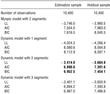
Table 2 Model Fit Statistics and Parameter Estimates
Estimation sample Holdout sample
Number of observations 10,400 10,400
Myopic model with 2 segments:
LL −3�746�0 −3�960�5
AIC 7�554�0 7�983�0
BIC 7�616�5 8�045�5
Dynamic model with 1 segment:
LL −4�024�3 −4�266�4
AIC 8�080�6 8�564�8
BIC 8�112�9 8�597�1
Dynamic model with 2 segments:
LL −3�414�0 −3�664�8
AIC 6�890�0 7�391�6
BIC 6�952�5 7�454�1
Dynamic model with 3 segments:
LL −3�401�1 −3�650�9
AIC 6�894�2 7�393�8
BIC 6�987�0 7�486�6
Notes.The numbers in bold denote best model fit. LL, log likelihood.
For estimating the model, we chose a random sam-ple of 400 customers.11 We used the first year of data
as an initialization period to compute the base hotel usage rate (BHU) and weekday stay (WDS) variables. Thus, there were 26 decision periods for each cus-tomer during the one-year time frame used in the esti-mation. In our data, about 98% of customers cashed in at least once during the two-year period; 72% cashed in exactly once. About 75% of customers had an initial points “inventory” of at least 10,000 points.
4. Results
4.1. Fit and Holdout Prediction
We estimated four models: (1) a myopic model with two latent segments, (2) a dynamic model with one segment, (3) a dynamic model with two segments, and (4) a dynamic model with three segments. The discount factor � in Equation (9) is set to 0 in the myopic model, whereas it is set at a biweekly equiv-alent of 0.995 in the dynamic model (Lewis 2004, Sun 2005). Fit statistics for the four models are provided in Table 2. The two-segment dynamic model provides the best fit according to Akaike information criterion (AIC) and Bayesian information criterion (BIC).12
The superiority of the two-segment dynamic model is supported by its performance in a holdout sam-ple. We applied the model to 400 customers not used
11There is nothing about the algorithm that would preclude a larger
sample size, but with 400, the model took six to seven days to con-verge. This sample size is similar to other research using dynamic models (Erdem et al. 2008, 2005; Osborne 2007).
12The within-group correlation for the paid stay nest was 0.35,
and the correlation for the free-stay nest was 0.38, suggesting it is important to include the�imtterms in the model (Equation (2)).
Thi
s
file
is
p
ro
vide
d
fo
r
in
formationa
l
purpose
s
on
ly
an
d
m
ay
no
t
b
e
re
distributed.
in the estimation. To assign holdout customers to segments, following Kamakura and Russell (1989), we use the estimated proportions of the two seg-ments as our prior probability of segment member-ship (73.3% for the first segment and 26.7% for the second segment). We then update this probability for each customer by incorporating the likelihood of his or her decision sequence. Based on Cramer (1999), who advocates using the prior probability as the cut-off, we assigned customers to the segment for which their posterior probability of being in that segment is larger than the prior probability. This means we used a 73.3% prior probability as the cutoff for classify-ing someone in the price segment. The rest are then assigned to the second segment. The corresponding fit statistics are shown in Table 2. The two-segment dynamic model again performs best.
The superiority of the dynamic to the static model is also reflected in the number of significant coefficients (21 for the dynamic model, 15 for the static model) as well as the diagnostics from the coefficients that are significant. For example, there is no rewarded behav-ior effect for the myopic model, yet there is one for the price-oriented segment in the dynamic model. This makes sense and is consistent with previous research that has found rewarded behavior effects.
4.2. The Two-Segment Solution
Table 3 reports the parameter estimates and their t-values for the two-segment model. Interestingly, Segment 1 derives significant positive utility from a free stay and shows no significant preference for an upgrade, whereas Segment 2 prefers the upgrade and no significant preference for a free stay. This is con-sistent with differences in price sensitivity: Segment 1 is more price sensitive, especially in response to the focal brand’s prices. Segment 2’s preference for a lux-ury property is positive and significant, whereas for Segment 1, it is not significantly different from 0. Members of Segment 2 have significant positive coef-ficients for both levels of the customer tier program, whereas the coefficient for only the Diamond tier is significant for Segment 1.
Given the above observations, we label the first segment “price oriented” in that its members are more price sensitive and are more attracted to free stays. We label the second segment “service oriented” because its members derive positive value for both customer tiers, favor upgrades, and prefer a luxury hotel. Consistent with this interpretation, the service-oriented segment exhibits a positive coefficient for the weekday stay variable, suggesting that its mem-bers are more likely to be business travelers, whereas the price-oriented segment has a significant negative weekday stay coefficient, suggesting that its members
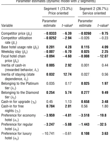
Table 3 Parameter Estimates
Parameter estimates (dynamic model with 2 segments)
Segment 1 (73.3%): Segment 2 (26.7%):
Price oriented Service oriented
Parameter Parameter
Variable estimate t-valuea estimate t-valuea
Competitor price (�0) −0�0333 −6�39 −0�0260 −9�75
Competitor utilization rate (�1�
−0�0252 −2�94 −0�026 −0�23
Base hotel usage rate (�2� 0�201 4�28 0�115 4�09
Weekday stay (�3� −0�007 −6�70 0�025 2�25
Focal hotel chain price (�4�
−0�094 −4�60 −0�008 −12�07 Inertia of cash-in
(rewarded behavior,�1)
0�005 2�92 0�001 0�44 Inertia of staying (state
dependence,�2)
0�032 12�74 0�027 0�56 Belonging to the Platinum
tier (�1�
0�035 0�17 0�025 1�97 Belonging to the Diamond
tier (�2�
0�254 5�74 0�277 9�49
Cash-in for upgrade (�0� 0�45 1�13 0�658 3�48
Cash-in for free nights��1�
0�784 2�01 0�56 1�80
Preference for economy hotel��1�
−3�959 −4�81 −3�518 −19�8 Preference for regular
hotel��2�
−3�247 −5�88 −1�443 −32�5 Preference for luxury
hotel��3�
−10�741 −0�61 0�108 3�63 aSignificant (p <0�05) estimates are indicated in bold.
are more likely to be leisure travelers.13 This is
con-sistent with the finding that Segment 1 is more price sensitive. The price-oriented segment is in the major-ity, 73.3%, of the sample, and the service-oriented seg-ment is 26.7%. Furthermore, there is support for the rewarded behavior effect for the price-oriented seg-ment, because�2is positive and significant. However, the rewarded behavior effect is not significant for the service-oriented segment.
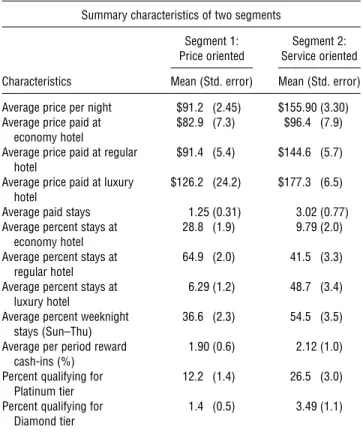
We provide further information on the price-oriented versus service-price-oriented segments in a hold-out sample (see Table 4). As expected, the service oriented segment pays a higher price (even when controlling for accommodation type), stays at a lux-ury hotel, and often qualifies for Diamond and Plat-inum tiers. Consistent with our observations above, the price-oriented segment is more likely to stay over the weekend.
Although not the focus of the paper, we close this section with a brief discussion of the competitive vari-able results. Tvari-able 3 shows that competitive price is
13Note we considered an alternative definition of the weekday
vari-able, allowing it to include Thanksgiving as well as Christmas as “weekend.” The results were invariant to this robustness check.
Thi
s
file
is
p
ro
vide
d
fo
r
in
formationa
l
purpose
s
on
ly
an
d
m
ay
no
t
b
e
re
distributed.
Table 4 Characteristics of Segments in Holdout Sample Summary characteristics of two segments
Segment 1: Segment 2:
Price oriented Service oriented
Characteristics Mean (Std. error) Mean (Std. error)
Average price per night $91�2 (2.45) $155�90 (3.30)
Average price paid at
economy hotel $82
�9 (7.3) $96�4 (7.9)
Average price paid at regular
hotel $91�4 (5.4) $144�6 (5.7)
Average price paid at luxury
hotel $126�2 (24.2) $177�3 (6.5)
Average paid stays 1�25 (0.31) 3�02 (0.77)
Average percent stays at
economy hotel 28�8 (1.9) 9�79 (2.0)
Average percent stays at
regular hotel 64�9 (2.0) 41�5 (3.3)
Average percent stays at
luxury hotel 6�29 (1.2) 48�7 (3.4)
Average percent weeknight
stays (Sun–Thu) 36�6 (2.3) 54�5 (3.5)
Average per period reward
cash-ins (%) 1�90 (0.6) 2�12 (1.0)
Percent qualifying for
Platinum tier 12
�2 (1.4) 26�5 (3.0)
Percent qualifying for
Diamond tier 1
�4 (0.5) 3�49 (1.1)
Note.Four hundred customers; 0.733 cutoff value.
significant in both segments, and occupation rate is significant for the price-oriented segment, with the expected signs. This suggests the value of including competitive data in the model. However, as noted earlier, these results must be taken as exploratory because our competitive variables are aggregates, and our “no-stay” option includes competitive stays as well as “non-stays.” These cross effects may therefore be underestimated.
4.3. Points Pressure Because of Loyalty Program Components
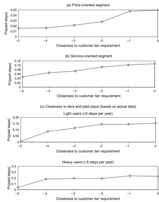
Points pressure refers to the buildup in purchase fre-quency as customers get closer to a reward. We find points pressure effects for both the frequency reward and customer tier components of the loyalty program. This is demonstrated in Figures 2(a)–2(c) and Fig-ures 3(a)–3(c), where we use simulations of the model as well as the raw data to calculate the probability of a paid stay (i.e., choosingm=1 andn=1�2�3� or 4) as the customer gets closer to earning the reward.
In Figures 2(a) and 2(b), the simulation begins with customers assigned to one of the two segments. We then assume each of them is five stays away from the next tier and estimate the probability of a paid stay. We do this for 5�4� � � � �0 stays away. We then plot the averaged simulated probability of a paid stay versus the closeness of the customer to the next tier
level. Figures 2(a) and 2(b) show that both segments increase their likelihood of paid stays as they get closer to earning membership in the next tier.14
These results are driven by the positive estimated coefficient (� >0) for customer tier membership. The points pressure behavior can be explained by the dynamic decision process: when the accumulated inventory is getting close to the next threshold, the rewards of higher tier membership can be attained sooner and hence are less discounted. As a result, total long-term utility of purchasing is higher, and customers purchase more.
Although tier classification is based onprevious pur-chase levels, an alternative explanation for the finding of points pressure is that tier membership is a proxy for high usage. Our base hotel usage rate variable con-trols for this because it reflects the number of stays in the initialization period. However, given the impor-tance of the issue, we include Figure 2(c), model-free evidence of the points pressure effect. To create this figure, we divide customers into heavy versus light users and calculate using the actual data the percent-age of paid stays on the y axis and the closeness to the next tier level on the x axis. The points pressure effect is apparent. This suggests that tier effects are real and not a reflection of the individual usage rate.15
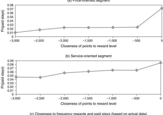
Using the same method as for the customer tier graphs, we investigated points pressure effects for the frequency reward program. Figures 3(a) and 3(b) are based on model-calculated probabilities of paid stay. Per the parameter estimates, we conclude that the points pressure for the price-oriented segment is driven by the free cash-in stays, and upgrades drive it for the service-oriented segment. Figure 3(c) is based on actual data, and akin to Figure 2(c), it provides model-free evidence of points pressure because of the frequency reward program. As in the case of customer tier, the probability of paid stays increases when reach-ing the reward level, now because of the high utility of a free upgrade as well as higher future utility.
Although points pressure has been demonstrated by previous research, that evidence was with respect
14Note that when customers reach the next tier (i.e., zero stays
away), their stay probability further increases because of the follow-ing: there is an increase in their utility because of the added benefits, and they continue to accumulate points for the next higher tier.
15In this calculation, it is possible that different customers are
included in different closeness states. To investigate this, we also performed the calculation for customers who were in each of the closeness states at least once during the data. We calculated the average probability of paid stay for each customer in each state and then averaged those averages across customers and plotted close-ness to the next tier versus probability of paid stay. The graphs showed the same increasing pattern as in Figure 2, as well as in Figure 3, for the frequency reward component.
Thi
s
file
is
p
ro
vide
d
fo
r
in
formationa
l
purpose
s
on
ly
an
d
m
ay
no
t
b
e
re
distributed.
Figure 2 The Points Pressure Effect Because of the Customer Tier Component
(a) Price-oriented segment
(b) Service-oriented segment
(c) Closeness to tiers and paid stays (based on actual data) Light users (≤5 stays per year)
Heavy users (>5 stays per year) 0 0.01 0.02 0.03 0.04 0.05 –5 –4 –3 –2 –1 0 Pr(paid stays)
Closeness to customer tier requirement
0 0.02 0.04 0.06 0.08 0.10 0.12 –5 –4 –3 –2 –1 0 Pr(paid stays)
Closeness to customer tier requirement
0 0.05 0.10 0.15 0.20 –5 –4 –3 –2 –1 0 Pr(paid stays)
Closeness to customer tier requirement
0 0.1 0.2 0.3 0.4 –5 –4 –3 –2 –1 0 Pr(paid stays)
Closeness to customer tier requirement
Note. Panels (a) and (b) are based on simulations assuming no frequency reward program.
to frequency rewards. Our finding is that points pres-sure exists for both frequency reward and customer tier components of a loyalty program.
4.4. Comparison to Two Separate Models for Frequency Reward and Customer Tier
One of the important research questions we aim to address with this research is the value of jointly modeling the frequency reward and customer tier components of loyalty programs, as opposed to modeling them separately. One obvious advantage of the joint approach is that we can predict changes in demand depending on simultaneous changes in the points requirement for both components. We will dis-cuss these analyses in §5. However, to further address this issue, we estimated two additional models.
1. Only frequency reward program: In this case, we removed the two customer tier variables (Platinum and Diamond) from the model and reestimated it.
2. Only customer tier program: In this case, we removed the frequency reward variables (free night, free upgrade, and inertia of cash-in) and reestimated the model.
We first find that the fit of the combined model (accounting for the number of parameters) is much better than the fit of either the frequency reward-alone model or customer tier-alone model (BIC=6�953 for combined model, 8,134 for customer tier-alone model, 8,941 for frequency reward-alone model). Clearly, if a research is modeling just one of the components, there is ample explanatory power to be gained by including the other as well.
Thi
s
file
is
p
ro
vide
d
fo
r
in
formationa
l
purpose
s
on
ly
an
d
m
ay
no
t
b
e
re
distributed.
Figure 3 The Points Pressure Effect Because of the Frequency Reward Component (a) Price-oriented segment
(b) Service-oriented segment
(c) Closeness to frequency rewards and paid stays (based on actual data) Light users (≤5 stays per year)
Heavy users (>5 stays per year)
0 0.01 0.02 0.03 0.04 0.05 0.06 0.07 0.08 –3,000 –2,500 –2,000 –1,500 –1,000 –500 0 Pr(paid stays) Pr(paid stays) Pr(paid stays) Pr(paid stays)
Closeness of points to reward level
Closeness of points to reward level
Closeness of points to reward level
Closeness of points to reward level
0 0.01 0.02 0.03 0.04 0.05 0.06 0.07 0.08 0.09 –3,000 –2,500 –2,000 –1,500 –1,000 –500 0 0.025 0.030 0.035 0.040 0.045 0.050 –2,500 –2,000 –1,500 –1,000 –500 0 0.06 0.11 0.16 –2,500 –2,000 –1,500 –1,000 –500 0
Note. Panels (a) and (b) are based on simulations assuming no customer tier program.
In addition, the diagnostics from the various models are different. For example, the competitive price variable is significant for only one segment among the four total segments in the customer tier-alone and frequency reward-tier-alone models, whereas this variable is significant for both segments in the combined model. The combined model sensi-bly suggests competitive prices are important for both segments. As another example, in the frequency
reward-alone model, the coefficients pertaining to the frequency reward program—inertia of cash-in, cash-in for upgrade, and cash-in for free nights—are all larger than their corresponding coefficients in the combined model, suggesting they may be overestimated in the separate models. As Table 4 shows, there is a positive association between membership in higher tiers and cash-in. Omitting tier membership therefore (mistak-enly) ascribes more importance to cash-in.
Thi
s
file
is
p
ro
vide
d
fo
r
in
formationa
l
purpose
s
on
ly
an
d
m
ay
no
t
b
e
re
distributed.
In summary, modeling the two components together produces better explanatory power and more sensible diagnostics compared to modeling the com-ponents separately. In the next section, we show how the combined model can be used to make predic-tions as we change the points requirement for both components.
5. Policy Implications
5.1. Overall Impact of Loyalty Programs on Customer Behavior and Firm Revenues
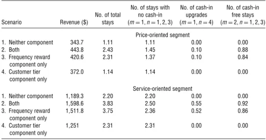
We simulate the model to investigate the over-all impact of the frequency reward and customer tier components of the loyalty program. We use the parameters in Table 3 to simulate four sce-narios: (1) the hotel employs neither the frequency reward nor the customer tier component, (2) the hotel employs both frequency reward and customer tier components, (3) the hotel employs the frequency reward but not the customer tier component, and (4) the hotel employs the customer tier but not the frequency reward component. For each scenario, we simulate customer behavior for a year and record stays and revenues per customer. The number of stays without cashing in is calculated as the average, over customers and time periods, of the probability of choosing m=1 and n=1�2, or 3, i.e., stay without cashing in. Similarly, we calculate the expected num-ber of upgrades (m=1 and n=4) and free stays (m=2 andn=1, 2, or 3). The results are presented in Table 5 and yield several conclusions.
First, both components generate incremental paid stays. This is particularly important for the frequency component, where one might conjecture that free stays would substitute for paid stays. However, this does not occur because the reward generates points
Table 5 Simulated Annual Stays, Cash-ins, and Upgrades per Customer Under Different Program Scenarios
No. of stays with No. of cash-in No. of cash-in
No. of total no cash-in upgrades free stays
Scenario Revenue ($) stays (m=1� n=1�2�3) (m=1� n=4) (m=2� n=1�2�3)
Price-oriented segment 1. Neither component 343�7 1�11 1�11 0�00 0�00 2. Both 443�8 2�43 1�45 0�10 0�88 3. Frequency reward 420�6 2�31 1�37 0�10 0�84 component only 4. Customer tier 372�0 1�14 1�14 0�00 0�00 component only Service-oriented segment 1. Neither component 1�189�3 2�20 2�20 0�00 0�00 2. Both 1�598�6 3�83 2�50 0�55 0�92 3. Frequency reward 1�511�8 3�75 2�36 0�52 0�86 component only 4. Customer tier 1�251 2�31 2�31 0�00 0�00 component only
pressure in anticipation of the reward and then a rewarded behavior carryover after the cash-in. Both these factors increase paid stays. Focusing on the price-oriented segment under the frequency reward-alone scenario, the annual number of paid stays per customer with no cash-in increases from 1.11 to 1.37, and the number of cash-in upgrades increases from 0.00 to 0.10. Thus the total increase is 0.36. The same calculation for the service-oriented segment reveals the total increase is 0.68.
Second, there is no cannibalization between the pro-grams; i.e., they do not cannibalize sales that would have occurred anyway. In fact, there may be some synergy, which can occur because both segments gain positive utilities from cashing in and elite status, and purchase probability is nonlinear in these utilities. Note that we are focusing on the revenue-generating aspects of these programs and do not take cost into consideration because of data limitations. For the service-oriented segment, the number of paid stays increase by 0.68 (2�88−2�20) when the frequency pro-gram is offered alone and by 0.11 (2�31−2�20) when the customer tier program is offered alone. If there was neither substitution nor complementarity, with both programs, the total number of paid stays would be 2�20+0�68+0�11=2�99. However, the number is a bit higher (3�05=2�50+0�55). The corresponding numbers for the price-oriented segment are 1.50 and 1.55. These synergy effects are not huge but certainly show that the components do not cannibalize each other and show how the model can be used to mea-sure these interactions.
Third, both segments respond to the customer tier program. This can be seen by comparing the base case scenario to the customer tier-alone scenario. For the price-oriented segment, the simulated number of
Thi
s
file
is
p
ro
vide
d
fo
r
in
formationa
l
purpose
s
on
ly
an
d
m
ay
no
t
b
e
re
distributed.
total stays per customer annually increases from 1.11 to 1.14. For the service-oriented segment, the num-ber of stays increases from 2.20 to 2.31.16 This is
because both segments have positive coefficients for the customer tier program and a positive points pres-sure effect as customers endeavor to build up points toward a higher tier. Fourth, both segments respond to the frequency reward program but for different reasons. The price-oriented segment is directly moti-vated to achieve free stays because of its large, signifi-cant coefficient. The service-oriented segment is more motivated by upgrades. However, for an upgrade to happen, the utility for an upgrade has to overcome the negative price effect of a purchase, whereas no such price effect exists for a cash-in free stay. So we find the service-oriented segment compiles both free stays and upgrades.
Fifth, although both components increase paid stays, the frequency component has a stronger impact than the customer tier program. This is especially true for the price-oriented segment, but even for the service-oriented segment. As we noted before, this segment will still cash in for free stays because although it is not as price sensitive as the price-oriented segment, it still is somewhat price sensitive, and a free stay saves a lot of money.
In summary, we find thatbothcomponents generate incremental sales and do not cannibalize each other. If anything, there is some synergy between them. These results of course are a function of our specific estimates and invite further research to generalize. We will take one step in that direction with our sec-ond application. The key point is that the dynamic structural model can be used to evaluate crucial issues involving the impact of these components.
5.2. Frequency Reward and Customer Tier Program Requirements to Increase Revenues
Here, we explore how a firm could use the model to adjust the requirements of its loyalty program to increase revenues. Two important notes before proceeding: First, the forthcoming scenarios do not consider competitive response. This is certainly a limitation, and although the data requirements would be daunting, our hope is that future research can model consumer response to competitive loyalty pro-grams. Second, one could raise the interesting ques-tion of why there should be a need to do this. We are assuming the customer is a sophisticated dynamic optimizer—surely, the firm should be as sophisti-cated. But our view is that in order for the firm to
16Note the baseline sales level for the service-oriented segment
(2.20) is greater than that for the price-oriented segment (1.11). This is due to lower alternative-specific constants for the price-oriented segment.
improve the effectiveness of its marketing mix, it must first understand how its customers respond to loy-alty programs. Then the firm can adjust. In this sense, the firm is a first mover—it tunes the loyalty pro-gram requirements taking into account the optimal customer response to these requirements. Note also that we are considering firm revenues, not profits.
Revenues can be increased by setting program requirements correctly, but this is a nontrivial task because there are many complexities and trade-offs. For example, if frequency reward requirements are lax, there will be minimal points pressure, but many cash-ins and hence ample rewarded behavior. If the requirements are tough, there will be more points pressure but not many cash-ins so less rewarded behavior. The optimal design will strike the right balance. The customer tier program presents simi-lar challenges. If the requirements are too lax, there is not much points pressure, but once the customer reaches a tier, paid stays increase because the cus-tomer receives continuously better service. If the requirements are too tough, we get more points pres-sure, but it takes customers longer to reach a tier, and many may not make it.
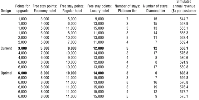
We conduct a grid search and simulations to determine the frequency reward and customer tier requirements that would most improve revenue per customer. We varied the free upgrade requirement from 1,000 points to 7,000, the free stay requirement at economy, regular, and luxury properties from 3,000, 5,000, and 7,000 points, respectively, to 15,000, all in steps of 1,000. Furthermore, we also varied the paid stay requirement for Platinum and Diamond tiers from 1 and 4, respectively, to 20 in steps of 1. In each cell, we simulated the behavior of 200 con-sumers. Table 6 presents the results for a subset of the design cells.
We find that although lower requirements encour-aged more staying, this reduces revenue, primarily because of free cash-in stays. For example, when the point requirements for an upgrade and free stays at the three types of properties are 1,000, 3,000, 5,000, and 9,000, respectively, the annual revenue per cus-tomer is only $544.70. On the other hand, the rev-enue increases to $558.10 for the current requirements of 3,000, 5,000, 8,000, and 12,000 for the reward pro-gram and 5 and 12 paid stays for the customer tier. The revenue-maximization setting (with an average annual revenue of $608.30) is 6,000, 8,000, 10,000, and 14,000 for the reward program and 3 and 6 annual paid stays for the customer tier program. This is a bit more stringent for the reward program but takes advantage of the points pressure effect, whereas it is less stringent for the Platinum and Diamond tiers (because of significant positive utility for segments and because there is less direct cannibalization of paid