Semi-supervised Multi-feature Learning for Person Re-identification
Dario Figueira
‡, Loris Bazzani
†, H`a Quang Minh
† ‡ISR - Instituto Superior T´ecnico
Lisboa, Portugal
Marco Cristani
†, Alexandre Bernardino
‡, Vittorio Murino
† †Pattern Analysis & Computer Vision
Istituto Italiano di Tecnologia
Genova - Italy
Abstract
Person re-identification is probablythe open challenge for low-level video surveillance in the presence of a camera network with non-overlapped fields of view. A large num-ber of direct approaches has emerged in the last five years, often proposing novel visual features specifically designed to highlight the most discriminant aspects of people, which are invariant to pose, scale and illumination. On the other hand, learning-based methods are usually based on sim-pler features, and are trained on pairs of cameras to dis-criminate between individuals. In this paper, we present a method that joins these two ideas: given an arbitrary state-of-the-art set of features, no matter their number, dimen-sionality or descriptor, the proposed multi-class learning approach learns how to fuse them, ensuring that the fea-tures agree on the classification result. The approach con-sists of a semi-supervised multi-feature learning strategy, that requires at least a single image per person as training data. To validate our approach, we present results on differ-ent datasets, using several heterogeneous features, that set a new level of performance in the person re-identification problem.
1. Introduction
Re-identification is considered one of the fundamen-tal building blocks of any multi-camera automated video-surveillance system. In the presence of a wide-area camera network with non-overlapped fields of view (as in the case of airports, stadiums, train stations, etc.), it allows the as-sociation of different instances of the same person across different locations and times.
The most important family of re-identification ap-proaches, to which the proposed approach belongs, is called
Labeled Set Features/ views 1 10 Kernels HSV LBP MR8 Unlabeled Set Multi-Feature Learning HSV LBP MR8 BVT Lab HSV LBP MR8 BVT Lab HSV LBP MR8 BVT Lab BVT Lab
Figure 1. Overview of the proposed method. The features of each individual are extracted from labeled and unlabeled images. Then, kernels are computed for each feature and finally the multi-feature classifier is trained.
appearance-based, since it considers solely the visual as-pect of people. Appearance-based methods can be further partitioned in two groups:directandlearning-based. Direct approaches focus primarily on designing effective descrip-tors which are invariant to pose, illumination, and scale, by exploiting the morphological aspects of humans and their peculiar characteristics. In particular, body symmetries and textural properties seem to be the most effective cues to tinguish people [7, 8, 12, 11], along with the chromatic tribution. The idea of these approaches is to compute dis-tances among gallery and probe subjects, where a specific similarity measure has to be designed for each cue. The dis-tances are minimized to establish matches among probe and gallery subjects. Multiple features are empirically merged to enrich the signature of a person by a weighted aver-age of the single distances and/or their concatenation (e.g., [11, 19]).
At the other extreme, learning-based methods investigate the aspects which are kept across different fields of view
and which differentiate people the most. Specifically, bi-nary classifiers (e.g., [3, 26]) are usually trained on pairs of instances of the same person (positive class) and pairs of different subjects (negative class). This setup is computa-tionally demanding in real scenarios, because it requires a training set for each pair of cameras, composed by at least two images per person (one for each camera).
In this paper, we propose a learning-based solution that synthesizes the best aspects of both worlds : 1) it allows the exploitation of multiple features independently of their na-ture and, at the same time 2) it does not require training a classifier for each pair of cameras. Our approach casts re-identification as a semi-supervised multi-class recognition problem, where each class corresponds to the identity of one individual. In particular, we exploit the general framework of multi-view (multi-feature1 here) learning with manifold regularization in vector-valued Reproducing Kernel Hilbert Spaces (RKHS), recently proposed in [23]. In this setting, each feature is associated with a component of a vector-valued function in an RKHS. Unlike multi-kernel learning [4], all components of a function are forced to map in the same fashion,i.e., to distinguish in a coherent way the dif-ferent individuals. The desired final output is given by their combination, in a form to be made precise below, which is a fusion mechanism joining together the different features.
As depicted in Fig. 1, the proposed approach trains a classifier from a labeled (gallery) set ofPdifferent individ-uals, exploiting the structure of unlabeled data that can be the probe set or images acquired during tracking. In other words, it does not require to have inter-camera image pairs of the same person, but only a single labeled image per per-son. This makes our approach truly applicable in real sce-narios. In general, unlabeled data can be any acquired im-age, such as individuals that are not in the gallery set.
The proposed method is compared with several state-of-the-art approaches on several challenging benchmarks. In all of the experiments, we outperform other compet-ing methods, thereby demonstratcompet-ing the validity of our ap-proach, and encouraging further experiments with novel cues.
The remainder of the paper is organized as follows. In Sec. 2, we briefly review the related literature and our con-tribution with respect to the state of the art. Sec. 3 fully de-tails our method, along with the features considered in this work. Experiments are then reported in Sec. 4, and, finally,
conclusions and future perspectives are given in Sec. 5.
2. Related Work
Following the taxonomy introduced in [11] , appearance-based techniques can be divided into learning-based and
1We prefer to use the term multi-feature instead, because views mean
different images of the same person in the context of re-identification.
direct methods and into single-shot and multi-shot ap-proaches.
Learning-based techniques are characterized by the use of a training dataset of different individuals where the fea-tures and/or the policy for combining them are analyzed to ensure high re-identification accuracy. The underlying as-sumption is that the knowledge extracted from the training set generalizes to unseen samples. Binary Support Vec-tor Machines (SVM) [3], multi-class SVM [24], nearest neighbor classifier [20], partial least square reduction [28], boosting [6, 17], distance learning [5, 18, 32], descriptor learning [12], and ensemble RankSVM [26] have been cus-tomized for the re-identification problem.
Direct methods do not consider any training sets. These methods are usually focused on finding discriminant parts of the human appearance and manually designing fea-tures that perform very well on a particular re-identification scenario. The framed person is typically subdivided into horizontal stripes [13], symmetrical and asymmetri-cal parts [11], semantic parts [14, 15], regions clustered by color [31], concentric rings [33], or a grid of localized patches [8]. Several features can be extracted from these regions: color histograms or other statistics [13, 11, 15], maximally stable color regions [11], depth features [10], histogram of oriented gradients [28], Gabor and Schmid fil-ters [26], interest points [16], covariance matrices [5, 9], attributes [19] and Haar-like features [6] have been exhaus-tively tested in the literature.
Single-shot approaches focus on associating pairs of im-ages, each containing one instance of an individual (e.g., [20, 24, 26, 28]). Multi-shot methods employ multiple im-ages of the same person as probe and/or gallery elements (e.g., [8, 11, 14, 29, 27]). The assumption of the multi-shot methods is that individuals are tracked so that it is possi-ble to gather a lot of images. The hope is that the system will obtain a set of images that vary in terms of resolution, partial occlusions, illumination, poses, etc.
Our approach lies in the category of the single-shot learning-based methods. It differs from the related litera-ture for the following reasons: 1) In contrast to all other learning-based strategies, it is able to learn the appearance of the individuals just from one labeled sample and from the additional unlabeled data,e.g., images gathered during tracking. 2) It offers a principled manner to fuse together different modalities/features, enforcing coherence among them.
3. The Proposed Approach
The pipeline of the proposed method is depicted in Fig. 1. The feature descriptors of each individual in the la-beled andunlabeledsets are extracted from detected body parts. Then, the similarity between the descriptors is com-puted for each feature by mean of kernel matrices (see
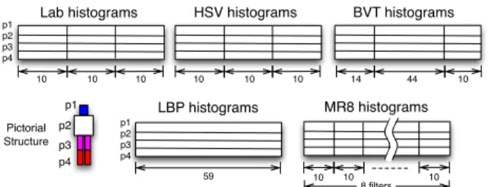
LBP histograms MR8 histograms BVT histograms HSV histograms Lab histograms p1 p2 p3 p4 p1 p2 p3 p4 p1 p2 p3 p4 Pictorial Structure 10 8 filters 10 10 10 10 10 10 10 10 14 44 10 59
Figure 2. Different features represented by blocks are computed from the detected parts{pi}4
i=1.
Sec. 3.1). Multi-feature learning consists in estimating the parameters of the model given the training set (see Sec. 3.2 and Sec. 3.3). Given a probe image, the testing phase con-sists in computing the similarity of each descriptor with the training samples and use the learned parameter to classify it (see Sec. 3.3).
3.1. Descriptors and Kernels
The first step of the algorithm is to frame the human ap-pearance in order to discard the background information that is considered noise for re-identification. In the same spirit of [14], the pictorial structure (PS) detector [2] is ap-plied to the images of each individual. Then, features are extracted from each of the four parts found by the detector (head, torso, upper-legs and lower-legs, see Fig. 2).
Two complementary aspects of the human appearance often used in the literature for re-identification [11, 12] are extracted from the images: the color distribution and the gradient patterns. For the former, the Black-Value-Tint (BVT) histograms used in [14] and the Hue Satura-tion Value (HSV) and Lightness color-opponent (Lab) his-tograms are adopted. For the latter, the Local Binary Pattern (LBP) histograms [25] and the histograms of the Maximum Responses filter banks (MR8) [30] are used. Fig. 2 shows the dimensionality of each feature and how they are con-catenated to generate each feature vector.
As described in Sec. 3.3, the learning algorithm requires computing a kernel matrix for each feature. Given the na-ture of the feana-tures, we used the Bhattacharyya kernel to compute similarity between samples, which usually shows good performance when dealing with histograms. Assume that each input vectorxcan be decomposed intomdifferent viewsx= (x1, . . . , xm)wherexj ∈
RCis thej-th feature
descriptor. Then the Bhattacharyya kernel of thei-th feature is defined as follows: ki(xi, ti) = exp −D(x i, ti) (σi)2 ! , (1) D(xi, ti) = v u u t1− C X c=1 p xi c·tic,
whereD(·,·)is the Hellinger distance between two distri-butions (normalized histograms), andσiis a parameter es-timated asσi=p
2·Di
med, whereD i
medis the median
dis-tance of the disdis-tance matrixD(xi, ti)given each(xi, ti)in
the training set.
3.2. Multi-feature Learning
The re-identification problem is defined in the multi-feature learning framework of [23], with theirviews corre-sponding to ourfeatures, as follows. Suppose that we have access to a training set {(xi, yi)}li=1 ∪ {xi}ui=+ll+1, where
xi∈ Xrepresents thei-th image of the individual with label
(identity)yi∈ Y. The first set is called the labeled set with lsamples while the second is the unlabeled set withu sam-ples, that is, whereyiis not available. In re-identification,
the labeled set corresponds to the gallery set and the unla-beled set can contain either the probe images or arbitrary images gathered during tracking. If the unlabeled set is not available, the method performs supervised learning.
Given that P is the number of identities in the re-identification problem, let the output space be Y = RP.
Each output label yi ∈ Y, 1 ≤ i ≤ l, has the form yi = (−1, . . . ,1, . . . ,−1), with1at thep-th location ifxi
is in thep-th class.
Let the number of features bem. LetW=Ym= RP m.
Let K : X × X → RP m×P m be a matrix-valued
posi-tive definite kernel that induces an RKHSHK of functions
f : X → W = RP m. For each function f ∈ HK,
f(x) = (f1(x), . . . , fm(x)), where fi(x) ∈ RP is the
value corresponding to theith feature.
The different features are fused together via a combina-tion operatorCas follows
Cf(x) = 1
m(f
1(x) +
· · ·+fm(x))∈RP. (2)
In terms of the Kronecker tensor product,Cis
C= 1
me T
m⊗IP, (3)
where IP is the P × P identity matrix and em =
(1, . . . ,1)T ∈
Rm. Other options to merge the different
features may be adopted, but we prefer to not introduce ad-ditional parameters that would have to be optimized during training.
Given the training set, re-identification consists of the following optimization problem based on the least square loss function: f?= argminf∈HK1 l l X i=1 ||yi−Cf(xi)||2Y +γA||f||2HK+γIhf, MfiWu+l (4)
withf = (f(x1), . . . , f(xu+l))and the regularization
pa-rametersγA >0andγI ≥0. The matrixM is defined as M =Iu+l⊗(Mm⊗IP), whereMm=mIm−emeTm[23].
The first term of Eq. 4 is the least square loss function that measures the error between the final outputCf(xi)for xiwith the given outputyifor eachi. The main difference
with the standard least square optimization in the first term is that this formulation combines the different features. In particular, if each input instancexhas many features, then
f(x) ∈ W represents the output values from all the fea-tures, constructed by their corresponding hypothesis spaces. These values are combined by the operator C to give the final output value inY. The second summand is the stan-dard RKHS regularization term. The third summand, multi-feature manifold regularization [23], performs consistency regularization across different features.
3.3. Solution of the Minimization Problem
The solution of the general minimization problem of Eq. 4 is reported in the following2. The problem has a unique solution f? = Pu+l
i=1Kxiai, where the vectors
ai∈ Ware given by the following system of equations:
(C∗CJlu+lK[x] +lγIM K[x] +lγAI)a=C∗y, (5)
wherea= (a1, . . . , au+l)is a column vector inWu+land y = (y1, . . . , yu+l)a column vector inYu+l. HereK[x]
denotes the(u+l)×(u+l)block matrix whose(i, j)block isK(xi, xj);Jlu+lis the block diagonal matrix of size(u+ l)×(u+l), with the firstlblocks on the main diagonal being
IWand the rest being0;C∗Cis the(u+l)×(u+l)block diagonal matrix, with each diagonal block beingC∗C;C∗
is the(u+l)×(u+l)block diagonal matrix, with each diagonal block beingC∗.
Assume that each input x is decomposed into x = (x1, . . . , xm)for themdifferent features. DefineK(x, t)
as a block diagonal matrix, with the(i, i)-th block given by
K(x, t)i,i=ki(xi, ti)IP, (6)
wherekiis a kernel of thei-th feature as defined in Sec. 3.1.
Define the matrixG[x]that contains all the kernels as (G(x, t))i,i=ki(xi, ti), (7)
andG[x]as the(u+l)×(u+l)block matrix, where each block(i, j)is the respectivem×mmatrixG(xi, xj).
Given this choice ofKandM =Iu+l⊗(Mm⊗IP),
the system of linear equations 5 is equivalent to
BA=YC, (8)
2For the derivations and the proofs of the equations contained in this
paper, we refer to the original paper [23].
where B = 1 m2(J u+l l ⊗emeTm) +lγI(Iu+l⊗Mm) G[x] +lγAI(u+l)m,
which is of size(u+l)m×(u+l)m,Ais the matrix of size(u+l)m×P such thata = vec(AT), andY
C is the
matrix of size(u+l)m×Psuch thatC∗y= vec(YT C).
Given the matricesBandYC, solving the system of
lin-ear equations 8 with respect toAis straightforward. There-fore, the learning method is simple to implement and is very efficient in practice.
Evaluation on a Testing Sample. Once A is thus computed, we need to estimate the labels/identities of the probe images v = {v1, . . . , vt} ∈ X. First, we compute f?(v
i)for each image, and compose the matrix f?(v) =
(f?(v1), . . . , f?(vt))T ∈RP mt, with f?(vi) = u+l X j=1 K(vi, xj)aj.
LetK[v,x]denote thet×(u+l)block matrix, where block (i, j)isK(vi, xj)and similarly, letG[v,x]denote thet×
(u+l)block matrix, where block(i, j)is them×mmatrix
G(vi, xj). Then
f?(v) =K[v,x]a= (G[v,x]⊗IP)a= vec(ATG[v,x]T).
In re-identification, vcontains the unlabeled samples,i.e.,
v={xi}ui=+ll+1.
For the i-th image of thep-th individual, f?(v i)
rep-resents the vector that is as close as possible to yi =
(−1, . . . ,1, . . . ,−1), with1at thep-th location. The iden-tity of thei-th image is estimateda-posterioriby taking the index of the maximum value in the vectorf?(v
i).
4. Experimental Evaluation
The experiments are carried out using public datasets to show that: 1) multi-feature learning increases the perfor-mance when adding multiple features, and 2) the proposed method outperforms other state-of-the-art techniques.
Datasets. We used standard challenging datasets for re-identification: iLIDS [33], VIPeR [17] and CAVIAR4REID [14]. iLIDS for re-identification [33] con-tains119people and was built from iLIDS Multiple-Camera Tracking Scenario. The challenges are the presence of oc-clusions and quite large illumination changes. VIPeR [17] contains two views of 632 pedestrians captured from dif-ferent viewpoints. CAVIAR4REID [14] contains images of pedestrians extracted from the CAVIAR dataset. It has a to-tal of72individuals:50with two camera views and22with one view. The individuals with one view are not considered in our experiments as in [14].
Table 1. Results on iLIDS (left) and VIPeR (right) datasets, comparing the single-feature and multi-feature learning. Best scores in bold, second best scores in italic.
iLIDS VIPeR Feature r= 1 r= 5 r= 10 r= 20 nAUC SFL LBP 11.60 27.06 38.66 53.44 74.36 MR8 12.19 31.85 44.12 55.71 78.75 Lab 24.87 46.81 54.71 65.63 83.42 HSV 24.37 45.55 55.88 66.13 83.27 BVT 26.89 47.48 56.22 66.64 83.96 MFL LBP+MR8 19.92 38.49 49.16 61.43 81.26 LBP+MR8+Lab 26.72 50.08 60.17 72.94 86.96 LBP+MR8+Lab+HSV 29.50 50.34 58.23 71.43 86.81 LBP+MR8+Lab+HSV+BVT 30.76 50.59 58.74 70.42 86.44 MFL opt. LBP+MR8+Lab+HSV+BVT 31.51 51.18 62.43 74.79 88.40 r= 1 r= 5 r= 10 r= 20 nAUC 1.68 7.56 11.71 20.63 66.93 2.02 8.13 12.82 22.85 73.46 11.17 28.51 36.90 48.51 85.68 17.94 38.42 51.99 66.14 91.61 16.71 34.71 46.30 58.32 88.73 3.39 10.06 17.72 28.23 76.56 10.38 24.87 35.35 47.56 85.48 18.01 37.44 48.73 62.34 91.89 19.59 40.76 52.21 66.11 92.34 22.53 44.40 55.92 70.70 93.75
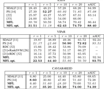
Table 2. Results on iLIDS (top), VIPeR (middle) and CAVIAR4REID datasets (bottom), comparing the proposed method with the state of the art. Best scores in bold, second best scores in italic. iLIDS r= 1 r= 5 r= 10 r= 20 nAUC SDALF [11] 28.49 48.21 57.28 68.26 84.99 PS [14] 27.39 52.27 60.92 71.85 87.08 [22] 25.97 43.27 55.97 67.31 83.14 [33] 24.00 43.50 54.00 66.00 − MFL 30.76 50.59 58.74 70.42 86.44 MFL opt. 31.51 51.18 62.43 74.79 88.40 VIPeR r= 1 r= 5 r= 10 r= 20 nAUC SDALF [11] 19.87 38.89 49.36 65.72 92.24 PS [14] 21.17 42.66 56.90 72.82 93.51 RDC [32] 15.66 38.42 53.86 70.09 − [21]+RankSVM [26] 15.73 37.66 51.17 66.27 − [21]+RDC [32] 16.14 37.72 50.98 65.95 − MFL 19.59 40.76 52.21 66.11 92.34 MFL opt. 22.53 44.40 55.92 70.70 93.75 CAVIAR4REID r= 1 r= 5 r= 10 r= 20 nAUC SDALF [11] 6.80 25.00 44.40 65.80 68.65 PS [14] 8.60 30.80 47.80 71.60 72.38 MFL 6.40 31.60 48.20 70.60 72.61 MFL opt. 8.20 35.20 53.20 74.00 74.39
Results. Standard metrics are used to evaluate the per-formance of the proposed method against the state of the art: the Cumulative Match Curve (CMC) and the normalized Area Under the CMC (nAUC). We pay particular attention to the first ranks of the CMCs,r={1,5,10,20}, because they better reveal the behavior of the methods in practice. The experiment protocol is consistent with the methods we compare with. Each dataset was randomly split10times in gallery and probe sets, and the results shows the average of the results over the different trials. In our experiments, the probe set is considered as unlabeled data.
We first tested the proposed re-identification method in a Single-Feature Learning setup (SFL in Table 1),i.e. the kernel of a single feature is used. Then, we added one fea-ture for each experiment to evaluate the increment in per-formance when including more features, that is the Multi-Feature Learning (MFL) in Table 1. For these
experi-ments, the regularization parameters are empirically set to
γI = 10−5andγA = 0.1and the kernel parameters (σi)
were estimated as noted in Sec. 3.1. In the last experiment (MFL opt. in Table 1), the regularization parameters along with the kernel parameters in Eq. 1 were optimized using the pattern search algorithm [1].
The results reported in Table 1 show the results on dif-ferent datasets: iLIDS on the left and VIPeR on the right. It is easy to notice that MFL is always better than the respec-tive single-feature experiment even when considering just two features. In fact, LBP+MR8 (sixth row) outperforms the SFL experiments of both LBP (first row) and MR8 (sec-ond row). The results show also that adding more features increases the accuracy. For the VIPeR dataset, the nAUC in-crease by15.78percentage points from the 2-feature to the 5-feature experiment. The best results are obtained when the parameters are optimized (MFL opt.).
Having demonstrated that the proposed MFL method is able to fuse different features, we now report the re-sults comparing it to the state-of-the-art learning-based and direct techniques proposed in last few years on different datasets. We show in Table 2 the results related to other re-identification techniques. MFL opt. outperforms all the methods in terms of nAUC and almost all the reported points of the CMC. PS is slightly better than MFL opt. in few points: r = {10,20} in VIPeR and r = 1 in CAVIAR4REID. In general, MFL opt. outperforms PS when considering the overall statistics on the CMC, such as the nAUC.
5. Conclusions
In this work, a semi-supervised multi-feature learn-ing framework has been proposed to deal jointly with the appearance-based and learning-based re-identification problem. Our solution poses re-identification as a multi-class recognition problem in a single-shot learning setup. An advantage of the presented technique is that it relies on a multi-feature learning framework to properly fuse differ-ent modalities and exploits the unlabeled data that are avail-able during tracking. The proposed method opens many
other interesting challenges, such as how to perform on-line learning to include new classes (individuals). Another point that should be investigated is a more complex loss function that considers the structure of the data and the correlation and differences across different classes.
Acknowledgments
This work was partially supported by FCT [PEst-OE/EEI/LA0009/2013] and by the project High Defini-tion Analytics (HDA), QREN - ID in Co-Promoc˜ao 13750, and by the project MAIS-S, CMU-PT / SIA / 0023 / 2009 under the Carnegie Mellon-Portugal Program. The work of Dario Figueira was partially supported with grant SFRH/BD/48526/2008, from Fundac˜ao para a Ciˆencia e a Tecnologia.
References
[1] M. A. Abramson.Pattern search algorithms for mixed vari-able general constrained optimization problems. PhD thesis,
´
Ecole Polytechnique de Montr´eal, 2002.
[2] M. Andriluka, S. Roth, and B. Schiele. Pictorial structures revisited: People detection and articulated pose estimation. InCVPR, 2009.
[3] T. Avraham, I. Gurvich, M. Lindenbaum, and S. Markovitch. Learning implicit transfer for person re-identification. In ECCV Workshops, 2012.
[4] F. R. Bach, G. R. G. Lanckriet, and M. I. Jordan. Multiple kernel learning, conic duality, and the SMO algorithm. In ICML, 2004.
[5] S. Bak, G. Charpiat, E. Corvee, F. Bremond, and M. Thon-nat. Learning to match appearances by correlations in a co-variance metric space. InECCV, 2012.
[6] S. Bak, E. Corvee, F. Bremond, and M. Thonnat. Person Re-identification Using Haar-based and DCD-based Signature. InAMMCSS, 2010.
[7] S. Bak, E. Corvee, F. Bremond, and M. Thonnat. Person Re-identification Using Spatial Covariance Regions of Human Body Parts. InAVSS, 2010.
[8] S. Bak, E. Corvee, F. Bremond, and M. Thonnat. Multiple-shot human re-identification by mean riemannian covariance grid. InAVSS, 2011.
[9] S. Bak, E. Corvee, F. Bremond, and M. Thonnat. Boosted human re-identification using riemannian manifolds. Image Vision Comput., 30(6-7):443–452, June 2012.
[10] I. B. Barbosa, M. Cristani, A. Bue, L. Bazzani, and V. Murino. Re-identification with rgb-d sensors. InECCV, 2012.
[11] L. Bazzani, M. Cristani, and V. Murino. Symmetry-driven accumulation of local features for human characterization and re-identification. Computer Vision and Image Under-standing, 117(2):130 – 144, 2013.
[12] L. Bazzani, M. Cristani, A. Perina, and V. Murino. Multiple-shot person re-identification by chromatic and epitomic anal-yses.Pattern Recognition Letters, 2011.
[13] N. Bird, O. Masoud, N. Papanikolopoulos, and A. Isaacs. Detection of loitering individuals in public transportation areas. IEEE Trans. on Intelligent Transportation Systems, 6(2):167 – 177, 2005.
[14] D. S. Cheng, M. Cristani, M. Stoppa, L. Bazzani, and V. Murino. Custom pictorial structures for re-identification. InBMVC, 2011.
[15] D. Figueira and A. Bernardino. Re-Identification of Visual Targets in Camera Networks a comparison of techniques. In ICIAR, 2011.
[16] N. Gheissari, T. B. Sebastian, P. H. Tu, J. Rittscher, and R. Hartley. Person reidentification using spatiotemporal ap-pearance. InCVPR, 2006.
[17] D. Gray and H. Tao. Viewpoint invariant pedestrian recogni-tion with an ensemble of localized features. InECCV, 2008. [18] M. Kostinger, M. Hirzer, P. Wohlhart, P. Roth, and H. Bischof. Large scale metric learning from equivalence constraints. InCVPR, 2012.
[19] R. Layne, T. Hospedales, and S. Gong. Person re-identification by attributes. InBMVC, 2012.
[20] Z. Lin and L. S. Davis. Learning pairwise dissimilarity pro-files for appearance recognition in visual surveillance. In Advances in Visual Computing, 2008.
[21] C. Liu, S. Gong, C. Loy, and X. Lin. Person re-identification: What features are important? InECCV Workshops. 2012. [22] N. Martinel and C. Micheloni. Re-identify people in wide
area camera network. InCVPR Workshops, 2012.
[23] H. Q. Minh, L. Bazzani, and V. Murino. A unifying frame-work for vector-valued manifold regularization and multi-view learning. InICML, volume 28, pages 100–108, 2013. [24] C. Nakajima, M. Pontil, B. Heisele, and T. Poggio.
Full-body person recognition system. Pattern Recognition Let-ters, 36(9):1997–2006, 2003.
[25] T. Ojala, M. Pietikainen, and T. Maenpaa. Multiresolution gray-scale and rotation invariant texture classification with local binary patterns. IEEE Trans. Pattern Anal. Mach. In-tell., 24(7):971–987, 2002.
[26] B. Prosser, W. Zheng, S. Gong, and T. Xiang. Person re-identification by support vector ranking. InBMVC, 2010. [27] P. Salvagnini, L. Bazzani, M. Cristani, and V. Murino.
Per-son re-identification with a ptz camera: an introductory study. InICIP, 2013.
[28] W. R. Schwartz and L. S. Davis. Learning discriminative appearance-based models using partial least squares. In Proceedings of the XXII Brazilian Symposium on Computer Graphics and Image Processing, 2009.
[29] J. Sivic, C. L. Zitnick, and R. Szeliski. Finding people in repeated shots of the same scene. InBMVC, 2006.
[30] M. Varma and A. Zisserman. A statistical approach to texture classification from single images.IJCV, 2005.
[31] X. Wang, G. Doretto, T. B. Sebastian, J. Rittscher, and P. H. Tu. Shape and appearance context modeling. InICCV, 2007. [32] W. Zheng, S. Gong, and T. Xiang. Re-identification by rela-tive distance comparison. IEEE Trans. Pattern Anal. Mach. Intell., PP(99):1, 2012.
[33] W. S. Zheng, S. Gong, and T. Xiang. Associating groups of people. InBMVC, 2009.