Efficient Reinforcement Learning for Robots using
Informative Simulated Priors
Mark Cutler and Jonathan P. How
Abstract— Autonomous learning through interaction with the physical world is a promising approach to designing controllers and decision-making policies for robots. Unfortunately, learning on robots is often difficult due to the large number of samples needed for many learning algorithms. Simulators are one way to decrease the samples needed from the robot by incorporating prior knowledge of the dynamics into the learning algorithm. In this paper we present a novel method for transferring data from a simulator to a robot, using simulated data as a prior for real-world learning. A Bayesian nonparametric prior is learned from a potentially black-box simulator. The mean of this function is used as a prior for the Probabilistic Inference for Learning Control (PILCO) algorithm. The simulated prior improves the convergence rate and performance of PILCO by directing the policy search in areas of the state-space that have not yet been observed by the robot. Simulated and hardware results show the benefits of using the prior knowledge in the learning framework.
I. INTRODUCTION
Designing useful controllers for real robots can be dif-ficult and tedious. Reinforcement learning (RL) [1] is one method for autonomously developing controllers based on data collected while operating in the real world. While RL has shown significant promise and impressive results in some domains, such as robot locomotion [2], helicopter flight [3], [4], backgammon [5], and elevator control [6], RL has not yet, in general, been employed in mainstream robotics as a standard tool for controller design. One of the many reasons RL is difficult to apply to real robots is the large number of samples needed to explore the often high-dimensional continuous state spaces common to many robot platforms [7]. These samples become particularly burdensome to obtain when they come from the real world because robots are expensive, only run in real-time, often require direct human supervision, and are subject to hardware degradation and failure.
One common tactic for decreasing the number of real-world samples needed in robotic RL is to perform “men-tal rehearsal” [7], a technique whereby the learning agent generates samples for an RL algorithm through querying a simulation of the robot. Simulation learning samples are typically much less costly (financially and temporally) to obtain than samples from a real robot. Simulations typically capture some aspects of an environment accurately and can provide valuable information to augment real-world data [8], [9]. Unfortunately, even very complex simulations of robots
Mark Cutler and Jonathan How are with the Laboratory of Information and Decision Systems, Massachusetts Institute of Technology, 77 Mas-sachusetts Ave., Cambridge, MA, USA{cutlerm,jhow}@mit.edu
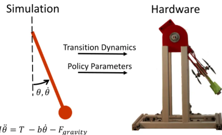
𝜃, 𝜃
𝐼 𝜃 = 𝑇 − 𝑏 𝜃 − 𝐹𝑔𝑟𝑎𝑣𝑖𝑡𝑦
Simulation
Hardware
Transition Dynamics Policy Parameters
Fig. 1: The proposed algorithm provides a method for transferring policies and learned transition dynamics from a simulated environment (left) to a real-world learning agent (right). The simulator captures the basic dynamics of the physical system but is not sufficiently accurate for performing learning in the simulator alone. Using policy parameters and transition dynamics learned in the simulator leads to faster learning on the physical robot. The algorithm is shown to decrease the number of samples needed by the real-world learning agent to achieve useful behavior.
rarely (if ever) perfectly model the real world, and imple-menting policies on a robot that were learned in an imperfect simulation can yield poor real-world performance [10].
There is significant existing work verifying the idea that using prior knowledge can increase the performance of learning algorithms. For instance, using a physics-based prior when learning inverse dynamics using a Gaussian process has been shown to yield superior performance when compared to using no prior knowledge [11], [12]. Also, several existing RL algorithms use simulators to augment real robot data [8], [9], [13]. Likewise, the transfer learning community [14] has sought to more seamlessly transfer information from simulators to the real world [15]. However, the above work assumes either an explicit form for the simulator equations or a discrete state and action space. In contrast, we leverage nonparametric Gaussian processes (GPs) to incorporate data from simulators in a principled way. The simulators can model continuous states and actions and be black-box codes such as proprietary robot simulators or based on finite element methods.
In this paper we introduce a method for using samples from a simulated robot to decrease the number of real-world samples that are needed to learn a good policy (see Figure 1). Specifically, we apply a learning algorithm in a simulator to learn a model of the simulated dynamics and a good policy for the simulated domain. The learned transition dynamics and policy are then used as a prior for real-world learning
us-ing the Probabilistic Inference for Learnus-ing Control (PILCO) algorithm [16]. The simulated prior is used in a GP model of the transition dynamics in PILCO to infer about states that the real-world system has not yet sampled. We show that, even when the simulator is inaccurate, using an informative simulated prior decreases the learning samples needed in the real world and increases the average performance of the achieved solution. Our approach differs from previous work using priors in PILCO[17] in that we are not limited to linear priors. Using a learned, nonlinear prior from a simulator allows for incorporating prior information from arbitrarily complex simulations without needing to make assumptions about the underlying dynamics of the system.
The main contributions of the paper are (1) a principled approach to incorporating data from any simulator into the PILCO learning algorithm, (2) a derivation of propagating uncertain inputs through a Gaussian process with a nonpara-metric mean function, and (3) simulated and hardware results empirically showing the benefits of using prior information in the learning process. Using prior data from a simple simulator, we show convergence to a good policy on a physical inverted pendulum with at least three times less data than is needed when a zero-mean prior is used.
The remainder of the paper is organized as follows. In Section II we recount some necessary background material on RL, the PILCO algorithm, and Gaussian processes. Sec-tion III details the derivaSec-tion of using a Gaussian process with a nonlinear mean when the inputs are uncertain. Sim-ulated and hardware results of the proposed algorithm are then shown in Section IV. Finally, we conclude with a brief discussion in Section V and summary in Section VI.
II. BACKGROUNDMATERIAL
In this section we briefly recount RL, the PILCOalgorithm, and
Gaussian processes.
A. Reinforcement Learning
The RL problem is modeled as a finite horizon Markov Decision Process [18], M =hS, A, R, Tiwith statesS and actions A. In this work we assume that both the states and the actions are real-valued vectors. The reward function R defines the quality of the current state by mapping the current state to a real number. In this work define the reward function as the negative of a user-defined cost function, such that R(s) = −c(s). The cost function is chosen to depend only on the current state and not the chosen action. The transition dynamics T map the probability of reaching state s0 as a function of the current state s and the current action a, so that T(s0, s, a) = p(s0|s, a). The goal of the RL algorithm
is to find a policy π∗ :s→a that minimizes the expected long-term cost J = H X t=0 Est[c(st)] (1)
over some fixed horizonH.
RL algorithms can be broadly classified as either model-based, where the algorithm explicitly builds a model of T which is in turn used to find π∗, or model-free, where π∗ is found without ever building a model of the transition dynamics. Model-based learners are generally more sample efficient but more computationally intensive than model-free approaches [19].
RL algorithms also differ as to how the optimal policy is found. Inpolicy searchmethods,π∗(θ)is parameterized by a vector θ and the RL algorithm searches for the optimal parameter values. In value-function methods, π∗ is instead found by keeping track of the estimated long-term cost of each state. Policy search methods are often advantageous as expert knowledge can easily be incorporated by specifying the form of the policy. Also, the number of parameters needed to optimize are usually fewer in policy search meth-ods than in corresponding value-function approaches [7].
B. PILCO
PILCO (Algorithm 1, black text) is a recently developed model-based policy search RL algorithm [16], [20], [21]. One of the key advantages of PILCOis a careful handling of uncertainty in the learned model dynamics that helps prevent negative effects of model bias. By explicitly accounting for uncertainty, the algorithm is able to determine where in the state space it can accurately predict policy performance and where more data are needed to be certain of future outcomes. As outlined in Algorithm 1, PILCO learns policy parameters in batches, or episodes. In each episode, the algorithm collects data from the target domain using the current policy parameters. The collected data are then used to learn a Gaussian process model of the transition dynamics. This model is used to update the policy parameters via an optimization routine such as CG or L-BFGS. Once the current policy parameters have converged, the target domain is rerun with the updated parameters and the process is repeated.
In this paper, as for the original PILCOalgorithm, we use empirical simulation and hardware results to verify the utility of the proposed algorithm.
C. Gaussian Processes
Gaussian processes (GPs) [22] are a popular regression tool for modeling observed data while accounting for uncer-tainty in the predictions, and are used to model the transition dynamics in PILCO. Formally, a GP is a collection of random variables, of which any finite subset are Gaussian distributed. A GP can be thought of as a distribution over possible functionsf(x),x∈ X such that
f(x)∼ GP(m(x), k(x,x0)), (2) where m(x) is the mean function and k(x,x0) is the
covariance function.
Algorithm 1 PILCO[16] with Prior Knowledge
1: input: Controller parameters, either random (θ ∼
N(0,I)) or from the simulator (θp). Apply random
control signals and record data.
2: input: Observed simulator data{Xp,yp} 3: Learn dynamics model using simulator data 4: while task not learneddo
5: Learn probabilistic (GP) dynamics model using real-world datawith the simulator data as a prior
6: while not convergeddo
7: Approximate inference for policy evaluation
8: Gradient-based policy improvement
9: Update parametersθ (e.g., CG or L-BFGS)
10: end while
11: return θ∗
12: Set π∗←π(θ)∗
13: Apply π∗ to system and record data
14: end while
distribution for a deterministic input x∗ is
f∗∼ N(µ∗,Σ∗) µ∗=m(x∗) +k(x∗, X)(K+σn2I)− 1(y −m(X)) =m(x∗) +k(x∗, X)β Σ∗=k(x∗,x∗)−k(x∗, X)(K+σ2nI)−1k(X,x∗) whereβ = (K+σ2nI)−1(y−m(X)), K=k(X, X), and σ2n is the noise variance parameter.
As in the PILCO algorithm [16], in this paper we use the squared error kernel for its computational advantages. Thus, the kernel is
k(x,x0) =α2exp(−1 2(x−x
0)TΛ−1(x
−x0)),
whereα2 is the signal variance andΛ is a diagonal matrix
containing the square of the length scales for each input di-mension. The hyperparmeters (σ2
n,α2, andΛ) are learned via
evidence maximization [22] (lines 3 and 5 of Algorithm 1). III. PILCO USING ANONLINEARPRIORMEAN
The generic PILCO algorithm assumes a zero-mean prior on the transition dynamics. This uninformative prior does not bias the model, giving the algorithm freedom to model arbitrary transition dynamics. However, the uninformative prior also means that the policy search algorithm cannot make informed decisions about areas of the state space from which no samples have yet been collected. In contrast, in this paper we propose using PILCOwith an informative prior consisting of data from a simulator of the real domain. The informative prior gives the policy search phase information about what effect a policy will have on the system even in areas of the state space that have not yet been explored. The proposed algorithm is shown in Algorithm 1, with the additions to the original algorithm highlighted in blue on lines 1-3 and 5.
The modified algorithm takes as inputs policy parameters (either randomly initialized or from a learning algorithm
applied to the simulator) and observed simulated data. The simulated data are used to build a probabilistic model of the simulator’s transition dynamics. The mean of this model is then used as a prior for the transition dynamics model learned in the target domain.
Given data from a simulation of the target domain, one way to incorporate the data into the learning algorithm is to train a single GP using both simulated and real data as inputs. Mixing simulated and real data has been shown to cause poor performance as the GP models of the real-world transition dynamics can become corrupted by incorrect simulation data [23]. In our approach, even with an incorrect simulator, real data from the target domain will eventually overcome the effects of the prior and converge to the true transition dynamics as the number of obtained data points increases.
To effectively use the learned GP dynamics model in PILCO (line 7 in Algorithm 1), the algorithm performs simulated roll-outs of the system dynamics using the learned model. This calculation requires machinery for correctly propagating the mean and covariance of uncertain inputs through the GP model of the transition dynamics. In this sec-tion we give the required calculasec-tions to propagate uncertain inputs through a GP when the prior function is the mean of a different GP. This mean prior function is equivalent to a radial basis function (RBF) network.
Unlike deterministic inputs, mapping an uncertain Gaus-sian test input x∗ ∼ N(µ,Σ) through a GP does not, in
general, result in a Gaussian posterior distribution. However, the posterior can be approximated as a Gaussian distribution by computing the mean and covariance of the posterior distribution [24]. PILCO iteratively uses these Gaussian ap-proximations when performing long-term predictions using the learned GP transition dynamics.
We now show the posterior mean and covariance equations when the prior mean of the GP is an RBF network. When the learning domain has multiple target variables (such as angle and angle rate for the inverted pendulum), independent GPs are learned for each output dimension. Where necessary, we differentiate between different output dimensions with subscripts a andb. In each equation, blue text denotes the terms that come from the prior. A full derivation of these equations is given in the Appendix.
The predictive meanµ∗ is given by
µ∗=βTq+βTpqp, (3)
where qi = α2|ΣΛ−1+I|−1/2exp(−12νTi(Σ + Λ)− 1)ν
i)
with νi =xi−µ. The subscript p denotes terms coming
from the prior.
The predictive covarianceΣ∗ of the uncertain test inputs
through the GPf(x)is given element-wise as σab2 =δab(α2a−tr((Ka+σ2aI) −1Q)) +βT aQβb+ βTp aQpβpb+β T pap ˆ Qβb+βTaQˆpβpb− βTaqa+β T paqpa β T bqb+β T pbqpb , (4)
Finally, PILCOuses the covariance between the uncertain test inputx∗∼ N(µ,Σ)and the predicted outputf(x∗)∼ N(µ∗,Σ∗) to compute the joint distribution p(x∗, f(x∗)).
This covariance is calculated as
Σx∗,f∗= n X i=1 βiqiΣ(Σ + Λ)−1(xi−µ)+ np X i=1 βpiqpiΣ(Σ + Λp) −1(x pi−µ). (5) In summary, Eq. (5)-(7) are the true predictive mean, covariance, and input-output covariance of an uncertain input passed through a GP with a mean function modeled as an RBF network.
In addition to propagating uncertain inputs through the transition dynamics model, PILCO requires the calculation of closed-form derivatives of the predicted mean, covariance, and input-output covariance with respect to the input mean and covariance. These calculations are rather long, but not particularly difficult and so are not included here. A full derivation of the required derivatives is given on the first author’s website.1
The computation of the predictive mean, covariance, and input-output covariance using a simulated prior requires approximately twice as much computation time as the zero-mean prior case (assuming the number of data points in the prior GP and the current GP are roughly equal), as most of the computations are merely repeated on the prior data. However, note that the size of the prior data is fixed and does not grow with iteration number, thus the additional computa-tional complexity of the algorithm due to the nonlinear prior does not grow as new data points are observed.
IV. RESULTS
Using the equations derived in the previous section, we perform both simulated and hardware experiments to identify how well the proposed alterations to PILCOwork in practice. In all of these experiments we run the generic PILCO
algorithm in the simulated domain and use the data collected during that learning exercise as the prior for the learning in the target domain. Note that any learning algorithm (including just randomly sampling the state-action space) could be applied in the simulator to obtain the required observations for the prior, but collecting data in the simulator using a good policy will more likely yield better results as data points will exist in the important areas of the state space. As in [16], we learn dynamics models using tuples
(xt,µt) as inputs and differences ∆t = xt+1−xt as
training targets. In all the experiments we also use the generalized binary saturating cost function from [16].
A. Using a Simulation Prior in a Simulated Domain The first set of results explore the performance of Al-gorithm 1 using two different simulations of the same domain. This will allow us to demonstrate the benefits of
1http://markjcutler.com/papers/Cutler15_ICRA_
additional.pdf
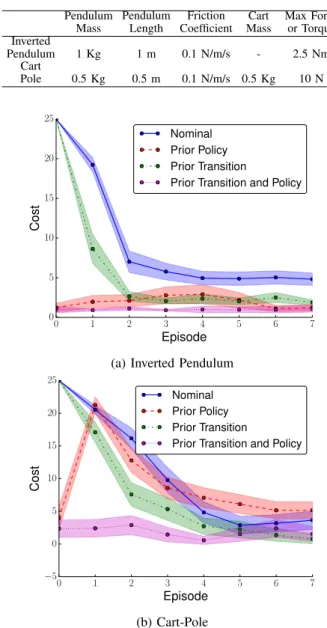
TABLE I: Default parameters used in the inverted pendulum and cart pole domains. Pendulum Mass Pendulum Length Friction Coefficient Cart Mass Max Force or Torque Inverted Pendulum 1 Kg 1 m 0.1 N/m/s - 2.5 Nm Cart Pole 0.5 Kg 0.5 m 0.1 N/m/s 0.5 Kg 10 N 0 1 2 3 4 5 6 7 Episode 0 5 10 15 20 25 Cost Nominal Prior Policy Prior Transition
Prior Transition and Policy
(a) Inverted Pendulum
0 1 2 3 4 5 6 7 Episode −5 0 5 10 15 20 25 Cost Nominal Prior Policy Prior Transition
Prior Transition and Policy
(b) Cart-Pole
Fig. 2: Learning curves for the 2-dimensional inverted pendulum (a) and the 4-dimensional cart-pole (b) domains when the prior comes from the same domain. Using an informative prior on the transition dynamics consistently improves performance regardless of the initial policy parameters. In the more complicated cart-pole domain using good initial policy settings does little to improve the algorithm performance unless prior transition information is used as well. Each line shows the mean of 20 independent learning samples each evaluated 5 times. The shaded regions show 95% confidence bounds on the standard error of the mean.
the algorithm as a function of the difference between the domains. The two chosen domains are the benchmark RL domains of the inverted pendulum and the inverted pendulum on a cart, or the cart-pole domain. Unless otherwise stated, the default parameters used for simulation of these domains are giving in Table I.
Using two identical instances of the target domains, we first verify that, given a perfect simulation of a physical robot (assuming such a simulation exists), no learning needs to be performed in the real-world as a learning algorithm can be applied in the simulator and the resulting control policy used
on the real robot. Figures 2(a) and 2(b) show the perfor-mance of Algorithm 1 under these idealized circumstances in the pendulum and cart-pole domains, respectively. In each figure the learning curves depict average cost as a function of learning episode. We compare (a) the original PILCO
algorithm with a random policy initialization, (b) the original PILCO algorithm using learned policy parameters from the simulation, (c) the proposed algorithm using a random policy initialization, and (d) the proposed algorithm using policy parameters from the simulation.
Note that, as expected, the learning curves either start with the performance of a random policy or with the performance of the converged policy, depending on the initial policy parameters used. When the prior policy is used and the prior for the transition dynamics comes from the same domain, the algorithm remains at the same performance level during the duration of the learning episodes as there is no incentive for the algorithm to explore different policy parameters. However, when a zero-mean prior is used (the original PILCO algorithm), even when initialized with near-optimal policy parameters, the performance actually gets worse for several learning episodes while the policy search explores different policy parameters before returning to the initial values. This transient learning phase is mild in the simple inverted pendulum domain. However, in the more complicated cart-pole domain, using a good prior policy does little to increase the learning rate when compared a random policy initialization.
In both domains, even when the algorithms are initialized with random policy parameters, using an informative prior speeds the learning process and consistently leads to a better policy. The on-average worse performance of the original PILCO algorithm comes from the algorithm occasionally converging to a sub-optimal solution. For instance, in the in-verted pendulum domain, the pendulum has sufficient torque to swing up to vertical with just one swing-back. However, the learning agent occasionally, depending on the random initial policy parameters, converges to a policy that consists of a double swing-back, taking longer than is necessary to get the pendulum to the inverted configuration. In these experiments, the prior data were generated using an instance of the PILCOalgorithm that converged to a single swing-back policy. Thus, even when the policy parameters are randomly initialized, having an informative prior coming from a good policy consistently helps the algorithm to converge to a single swing-back policy.
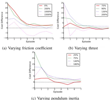
The next set of results demonstrates the performance of Algorithm 1 when the data for the prior come from a domain with different transition dynamics than the target domain. In Figures 3 and 4 the performance of PILCO using an informative prior (transition dynamics and policy parameters) is compared to using a uniform prior and random initial policy parameters. The plots show the difference between the uninformative and the informative prior as the domain parameters are varied between the prior domain and the target domain. For instance, in Figure 3(a) a prior learned in the default domain was used in a target domain where
0 1 2 3 4 5 6 7 Episode 10 5 0 5 10 15 20 25 Cost Difference 0% 200% 1000% 1500%
(a) Varying friction coefficient
0 1 2 3 4 5 6 7 Episode 10 5 0 5 10 15 20 25 Cost Difference 75% 90% 130% 200% (b) Varying thrust 0 1 2 3 4 5 6 7 Episode 5 0 5 10 15 20 25 Cost Difference 25% 75% 140% 180%
(c) Varying pendulum inertia
Fig. 3: Differences between the original PILCOalgorithm and the algorithm when using an informative prior in the pendulum domain. In each case the informative prior was learned using the nominal pendulum parameters in Table I and then tested in a domain where the default parameters were varied. Positive cost differences show the modified algorithm performing better than the original during that episode. Thus, except when the target domain was extremely different from the prior domain, the modified algorithm performed better than the original. Each line is the average of 24 independent learning runs. The error bars have been left off for clarity, but are similar in magnitude to those in Figure 2.
0 1 2 3 4 5 6 7 Episode 5 0 5 10 15 20 25 Cost Difference 0% 200% 1000% 1500%
(a) Varying friction coefficient
0 1 2 3 4 5 6 7 Episode 5 0 5 10 15 20 Cost Difference 75% 90% 130% 150% (b) Varying torque
Fig. 4: Results when varying the friction coefficient and the actuator force from the prior to the target domain in the cart-pole domain. As in the inverted pendulum (see Figure 3), the modified algorithm is robust to significant difference between the prior and the target domain.
the friction coefficient was up to 15 times more than the default value. In each plot, the parameters not varied were kept at their default values. Positive cost differences show the modified algorithm performing better than the original. Except for extreme changes in the parameters of the target domain compared to the prior domain, using an informative prior from an imperfect simulator is still better than using no prior at all.
Due to the nature of continuous state-action RL being an optimization problem in an arbitrary non-convex space, it is difficult, if not impossible, to quantify or predict the expected improvement of using a simulated prior in a domain as opposed to using a zero-mean prior. Intuitively, we should expect data from an arbitrarily poor simulator not to be
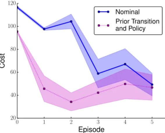
0 1 2 3 4 5 Episode 20 40 60 80 100 120 Cost Nominal Prior Transition and Policy
Fig. 5: Difference between PILCOwith a zero-mean prior and the proposed extension with a nonparametric prior coming from a simulator when implemented on a physical inverted pendulum. In the simulated prior both the dynamics and the policy are passed to the real domain. Each algorithm was run three times, with the policy at each episode evaluated 5 times. Error bars show a 95% confidence interval on the standard error of the mean. On average, the additional knowledge from the simulator led the physical system to converge to a good policy in just one episode, whereas without prior knowledge PILCOrequired at least three learning episodes before the pendulum could be stabilized.
useful, and possibly even be harmful to the learning process if it causes the gradient-based policy optimizer to look in the wrong directions. For instance, in Figure 3(b), when the true domain thrust is 200% higher than the simulated domain thrust, the optimal policies are fundamentally dif-ferent between the domains. The additional thrust allows the pendulum to go directly from hanging down to upright without a swing-back. The zero-mean prior algorithm dis-covers this simple policy after a single iteration; however, using the simulated prior, the learning is biased towards policies that use a swing-back to reach the goal position, temporarily causing worse performance. Further discussion on whether the proposed algorithm will improve the learning performance is contained in Section V.
B. Using a Simulated Prior on an Inverted Pendulum In this section we verify the performance of Algorithm 1 on a physical implementation of the inverted pendulum, shown in Figure 1. The pendulum is actuated using two propellers driven by independent brushless motors. The propellers are facing opposite directions, blowing air away from each other. The control input to the motors keep the propellers spinning at all times as brushless motors have a significant spin-up time when starting from rest. The angle and angle rate of the pendulum are estimated using on-board inertial sensors (rate gyro and accelerometer). These estimates are relatively low-noise and so are treated as truth in the learning process. Policy roll-outs are performed by sending policy parameters to the on-board microcontroller which, in turn, implements a nonlinear deterministic GP policy using the received parameters. Observed state values and control inputs are sent back to the host computer upon completion of the roll-out as the policy learning is not performed on-board the robot. The control is executed
at 20 Hz and each roll-out is 3 seconds long, giving 60 additional data points for each new policy update phase.
The prior comes from a very simple simulation of the physical pendulum with parameters such as mass, inertia, and commanded force roughly measured or estimated. Figure 5 shows a comparison of the proposed algorithm with both prior transition dynamics and initial policy parameters com-ing from the simulator. The simple simulator does not model physical effects such as aerodynamic interactions between the propellers or the change in generated torque as a function of angular rate. Thus, the initial policy parameters do not do much better than random control signals at stabilizing the system (episode 0 in Figure 5). However, with just 3 seconds of data from the initial policy roll-out, the proposed algo-rithm is able to consistently stabilize the pendulum. The zero-mean original PILCOalgorithm, on the other hand, requires on average at least 3 times as much data from the real system before a stabilizing controller is learned.
A video showing the performance of the hardware using the two algorithms can be found at http://youtu.be/ kKClFx6l1HY.
V. DISCUSSION
PILCO does not have exploration strategy guarantees but rather relies an exploration-exploitation strategy that emerges from the saturating cost function used in the experiments. While this strategy appears to work well in general, as shown in the previous section, in our experience PILCO
does not always converge to the global optimum. Even in simple problems such as the inverted pendulum the algorithm occasionally gets stuck in local minima. One advantage of the proposed modifications to the PILCO algorithm is the ability to apply any applicable learning strategy in the simulated domain and use the data to form a prior for the modified PILCOalgorithm. Also, since running the simulator is most likely much cheaper and easier than running the physical hardware, many learning instances could be run in the simulator before turning on the physical hardware.
In the results in the previous section we made sure to use data for the prior from a learning instance where the algorithm converged to near-optimal behavior. As such behavior will not, in general, be known beforehand in any giving learning setup, the prior could instead be chosen by repeatedly applying a learning algorithm in the simulator with varying initial conditions and then using the data from the best performance.
Note that using a simulated prior will not increase the algorithm performance in all cases. If the simulation is arbitrarily poor, the prior can bias the transition dynamics in the wrong directions. Given sufficient data from the target domain, the observed data will eventually overpower the prior. However, since PILCO is a policy search algorithm that follows local gradients, a poor prior can alter the policy search directions and lead to different policies than had no prior been used.
We also note that, as discussed in [10], applying policies learned in imperfect simulations can yield arbitrarily poor
performance, possibly even causing harm to the robot if the policy is overly aggressive. Thus, transferring the initial policy should be done with care. If there is danger of harming the robot, the prior dynamics model can be used with a random, or less aggressive, initial policy.
VI. CONCLUSION
We introduced a method for incorporating data from arbitrary simulators in the PILCO learning framework. The simulated data are used to learn a GP model of the simulated transition dynamics. The mean of these dynamics is then used as an informative prior for the real transition dynamics in the target domain. We derived the appropriate equations for predicting the mean and covariance of uncertain inputs using a GP with a mean modeled as an RBF network. The proposed extensions to the PILCO algorithm are demon-strated to result in faster and more robust convergence to good policies than the original PILCO algorithm. These results are shown in both simulated domains and on a physical inverted pendulum using a simple simulator.
APPENDIX
Here we derive Eq. (3)-(5) from Section III. Following the outline of the derivations in [16] and [17] the predictive mean of uncertain inputx∗∼ N(µ,Σ)is given by
µ∗= Ex∗,ff[f(x∗)] = Ex∗[Ef[f(x∗)]]
= Ex∗[k(x∗, X)β+m(x∗)]. (6)
We assume the prior mean functionm(x∗)is the mean of a
GP that is trained using data from a simulator. Thus,
m(x∗) =kp(x∗, Xp)βp
where {Xp,yp} are the simulated data, βp = (Kp +
σ2 npI)
−1(y
p−m(Xp)), Kp =kp(Xp, Xp), and σ2np is the noise variance parameter of the simulated data. Note that we assume that the prior mean is trained using a zero-prior GP. Substituting the form of the mean function into Eq. (6) yields
µ∗=βTq+βTpqp, (7)
whereqi=α2|ΣΛ−1+I|−1/2exp(−12νTi(Σ+Λ)− 1ν
i)with
νi=xi−µ. The corresponding prior terms are similar with
qpi = α 2 p|ΣΛ−p1+I|−1/2exp(−12ν T pi(Σ + Λp) −1ν pi) and νpi=xpi−µ.
Multi-output regression problems can be solved by train-ing a separate GP for each output dimension. When the inputs are uncertain, these output dimensions covary. We now compute the covariance for different output dimensionsaand b as
Covx∗,f[fa(x∗),fb(x∗)] = Ex∗[Covf[fa(x∗), fb(x∗)]]
+ Ex∗[Ef[fa(x∗)]Ef[fb(x∗)]]
−Ex∗[Ef[fa(x∗)]]Ex∗[Ef[fb(x∗)]]. (8)
As noted in [17], due to the independence assumptions of the GPs, the first term in Eq. (8) is zero when a 6= b. Also, for a given output dimension, Covf[fa(x∗), fb(x∗)]
does not depend on the prior mean function. Therefore, using the results of [16], the first term in Eq. (8) becomes
Ex∗[Covf[fa(x∗), fb(x∗)]] =
δab(α2a−tr((Ka+σ2aI)
−1
Q)), (9) whereδab is 1 whena=b and 0 otherwise, and
Q= Z ka(x∗, X)Tkb(x∗, X)p(x∗)dx∗ Qij =|R|−1/2ka(xi,µ)kb(xj,µ) exp(12zTijT −1z ij) (10) R= Σ(Λ−a1+ Λ−b1) +I T = Λ−a1+ Λ−b1+ Σ−1 zij = Λ−a1νi+ Λ−b1νj.
The third term in Eq. (8) is computed using Eq. (7) as
Ex∗[Ef[fa(x∗)]]Ex∗[Ef[fb(x∗)]] = βTaqa+βTp aqpa β T bqb+β T pbqpb . (11)
Finally, we compute the second term in Eq. (8) as
Ex∗[Ef[fa(x∗)]Ef[fb(x∗)]] =
Ex∗[k(x∗, X)βak(x∗, X)βb+ma(x∗)mb(x∗)+
ma(x∗)k(x∗, X)βb+k(x∗, X)βamb(x∗)]. (12)
As above, we will compute each term separately. Using Eq. (10), the first term in Eq. (12) becomes
Ex∗[k(x∗, X)βak(x∗, X)βb] =β T
aQβb. (13)
Similarly, the second term in Eq. (12) is
Ex∗[ma(x∗)mb(x∗)] =
Ex∗[kp(x∗, Xp)βpakp(x∗, Xp)βpb] =β
T
paQpβpb, (14)
whereQp is defined analogously to Eq. (10) but using the
prior rather than the current data. The third term in Eq. (12) is Ex∗[ma(x∗)k(x∗, X)βb] = βTp aEx∗[kp(Xp,x∗)k(x∗, X)]βb=β T pa( pQˆ)β b, (15) wherepQˆ is defined as pQˆ = Z kpa(x∗, Xp) Tk b(x∗, X)p(x∗)dx∗ pQˆ ij =|pRˆ|−1/2kpa(xpi,µ)kb(xj,µ)× exp(1 2( pzˆ ij)T(pTˆ)−1(pzˆij) (16) pRˆ = Σ(Λ−1 pa + Λ −1 b ) +I pTˆ= Λ−1 pa + Λ −1 b + Σ −1 pzˆ ij = Λ−pa1νpi+ Λ −1 b νj.
The forth term in Eq. (12) is analogously defined as βTaQˆpβpb, where ˆ Qp= Z ka(x∗, X)Tkpb(x∗, Xp)p(x∗)dx∗ ˆ Qpij=|Rˆp|−1/2ka(xi,µ)kpb(xpj,µ)× exp(12(ˆzpij)T( ˆTp)−1zˆpij) (17) ˆ Rp= Σ(Λ−a1+ Λ−p1 b) +I ˆ Tp= Λ−a1+ Λ−pb1+ Σ−1 ˆ zpij= Λ−a1νi+ Λ−pb1νpj.
Combining Eq. (9)-(17) we obtain the covariance for an uncertain input with multiple outputs. Writing this covariance element-wise we obtain σab2 =δab(α2a−tr((Ka+σ2aI) −1Q)) +βT aQβb+ βTpaQpβpb+β T pa pQˆβ b+β T aQˆ pβ pb− βTaqa+βTp aqpa β T bqb+β T pbqpb . (18)
The final derivation needed for propagating uncertain in-puts through the GP transition model in the PILCOalgorithm is the covariance between the uncertain test input x∗ ∼ N(µ,Σ)and the predicted outputf(x∗)∼ N(µ∗,Σ∗). This
covariance is calculated as Σx∗,f∗ =Ex∗,f[x∗f(x∗) T] −Ex∗[x∗]Ex∗,f[f(x∗)] T =Ex∗,f[x∗k(x∗, X)β]− Ex∗[x∗]Ex∗[k(x∗, X)β] T+ Ex∗,f[x∗kp(x∗, Xp)βp]− Ex∗[x∗]Ex∗[kp(x∗, Xp)βp] T.
Here we have separated the input-output covariance into a part that comes from the current data and a part that comes from the prior data. Therefore, we can directly apply the results from [16] to obtain
Σx∗,f∗=Σ(Σ + Λ) −1 n X i=1 βiqi(xi−µ)+ Σ(Σ + Λp)−1 np X i=1 βpiqpi(xpi−µ). (19)
Note that in the derivation above we do not assume that there are the same number of data points in the prior GP and the current GP. Thus, the matricespQˆ andQˆp need not be square.
ACKNOWLEDGMENT
This work was partially supported by the National Sci-ence Foundation Graduate Research Fellowship under grant No. 0645960. The authors acknowledge Boeing Research & Technology for support of the facility in which the experiments were conducted. The authors also thank Dr. Marc Deisenroth for his insightful feedback on the research.
REFERENCES
[1] R. Sutton and A. Barto,Reinforcement Learning, an Introduction. Cambridge, MA: MIT Press, 1998.
[2] N. Kohl and P. Stone, “Policy gradient reinforcement learning for fast quadrupedal locomotion,” in IEEE International Conference on Robotics and Automation (ICRA), 2004, pp. 2619–2624.
[3] A. Y. Ng, A. Coates, M. Diel, V. Ganapathi, J. Schulte, B. Tse, E. Berger, and E. Liang, “Autonomous inverted helicopter flight via reinforcement learning,” in Proceedings of International Symposium on Experimental Robotics, Singapore, June 2004.
[4] J. A. Bagnell and J. Schneider, “Autonomous helicopter control using reinforcement learning policy search methods,” inIEEE International Conference on Robotics and Automation (ICRA). IEEE, May 2001. [5] G. Tesauro, “Temporal difference learning and TD-Gammon,”
Com-mun. ACM, vol. 38, no. 3, pp. 58–68, 1995.
[6] A. Barto and R. Crites, “Improving elevator performance using reinforcement learning,” Advances in neural information processing systems, vol. 8, pp. 1017–1023, 1996.
[7] J. Kober, J. A. Bagnell, and J. Peters, “Reinforcement learning in robotics: A survey,”The International Journal of Robotics Research, vol. 32, no. 11, pp. 1238–1274, 2013.
[8] P. Abbeel, M. Quigley, and A. Y. Ng, “Using inaccurate models in reinforcement learning,” inInternational Conference on Machine Learning (ICML), 2006, pp. 1–8.
[9] J. Z. Kolter and A. Y. Ng, “Policy search via the signed derivative,” inRobotics: Science and Systems (RSS), Seattle, USA, June 2009. [10] C. G. Atkeson and S. Schaal, “Robot learning from demonstration,”
inInternational Conference on Machine Learning (ICML), 1997, pp. 12–20.
[11] D. Nguyen-Tuong and J. Peters, “Using model knowledge for learning inverse dynamics,” inRobotics and Automation (ICRA), 2010 IEEE International Conference on. IEEE, 2010, pp. 2677–2682. [12] J. Ko, D. Klein, D. Fox, and D. Haehnel, “Gaussian processes and
reinforcement learning for identification and control of an autonomous blimp,” inRobotics and Automation, 2007 IEEE International Con-ference on. IEEE, 2007, pp. 742–747.
[13] M. Cutler, T. J. Walsh, and J. P. How, “Reinforcement learning with multi-fidelity simulators,” inIEEE International Conference on Robotics and Automation (ICRA), Hong Kong, 2014, pp. 3888–3895. [14] M. E. Taylor, P. Stone, and Y. Liu, “Transfer learning via inter-task mappings for temporal difference learning,”Journal of Machine Learning Research, vol. 8, no. 1, pp. 2125–2167, 2007.
[15] T. A. Mann and Y. Choe, “Directed exploration in reinforcement learning with transferred knowledge,” in European Workshop on Reinforcement Learning, 2012, pp. 59–76.
[16] M. Deisenroth, D. Fox, and C. Rasmussen, “Gaussian processes for data-efficient learning in robotics and control,”Pattern Analysis and Machine Intelligence, IEEE Transactions on, vol. PP, no. 99, 2014. [17] B. Bischoff, D. Nguyen-Tuong, H. van Hoof, A. McHutchon, C.
Ras-mussen, A. Knoll, J. Peters, and M. Deisenroth, “Policy search for learning robot control using sparse data,” inIEEE International Conference on Robotics and Automation (ICRA). Hong Kong: IEEE, June 2014.
[18] M. L. Puterman, Markov Decision Processes: Discrete Stochastic Dynamic Programming. New York, NY: John Wiley & Sons, Inc., 1994.
[19] I. Szita and C. Szepesv´ari, “Model-based reinforcement learning with nearly tight exploration complexity bounds,” in International Conference on Machine Learning (ICML), 2010, pp. 1031–1038. [20] M. Deisenroth and C. E. Rasmussen, “Pilco: A model-based and
data-efficient approach to policy search,” inProceedings of the 28th International Conference on Machine Learning (ICML-11), 2011, pp. 465–472.
[21] M. P. Deisenroth, Efficient reinforcement learning using gaussian processes. KIT Scientific Publishing, 2010, vol. 9.
[22] C. Rasmussen and C. Williams, Gaussian Processes for Machine Learning. MIT Press, Cambridge, MA, 2006.
[23] D. Meger, J. C. G. Higuera, A. Xu, and G. Dudek, “Learning legged swimming gaits from experience,” inIEEE International Conference on Robotics and Automation (ICRA). Seattle, WA: IEEE, 2015. [24] A. Girard, C. Rasmussen, J. Q. nonero Candela, and R.
Murray-Smith, “Gaussian process priors with uncertain inputs — application to multiple-step ahead time series forecasting,” inAdvances in Neural Information Processing Systems 15 (NIPS), 2005.