Computational Optimization Methods in Statistics, Econometrics and Finance
COMISEF WORKING PAPERS SERIES
WPS-038 17/05/2010
J. Zhang
W. L. Ng
-Exact Maximum Likelihood Estimation for
Copula Models
Jin Zhang
∗Wing Long Ng
†Abstract
In recent years, copulas have become very popular in financial research and actuarial science as they are more flexible in modelling the co-movements and relationships of risk factors as compared to the conventional linear cor-relation coefficient by Pearson. However, a precise estimation of the copula parameters is vital in order to correctly capture the (possibly nonlinear) dependence structure and joint tail events. In this study, we employ two optimization heuristics, namely Differential Evolution and Threshold Ac-cepting to tackle the parameter estimation of multivariate t distribution models in the EML approach. Since the evolutionary optimizer does not rely on gradient search, the EML approach can be applied to estimation of more complicated copula models such as high-dimensional copulas. Our experimental study shows that the proposed method provides more robust and more accurate estimates as compared to the IFM approach.
Key words. Copula Models, Parameter Inference, Exactly Maximum Likelihood, Differential Evolution, Threshold Accepting.
1
Introduction
Nowadays, copulae have been widely applied by practitioners to model the de-pendence structure of financial risk factors, such as equities and exchange rates. The popularity of copulae is mainly due to their flexibility as they can be used to model both the linear and non-linear dependence structure of a multivariate dis-tribution. The linear correlation by Pearson is not only insufficient in describing the dependence of risk factors which moving away from elliptical distributions, but
∗Centre for Computational Finance and Economic Agents, University of Essex, United
King-dom. [email protected]
†Centre for Computational Finance and Economic Agents, University of Essex, United
also inconsistent under nonlinear strictly increasing transformations of risk factors (see McNeil et al. [2005]). Therefore, using copula-based dependence measures will be more accurate in capturing the dependence structure than calculating the linear correlation.
However, a precise estimation of parameters in copula models is crucial to de-pendence modelling. In the literature, several ways based on the statistical infer-ence theory were developed to estimate the parametric and non-parametric copula models (see Joe [1997]). These approaches can be mainly classified into three types: parametric approaches (e.g. the maximum likelihood estimation), semi-parametric estimation and non-semi-parametric methods. The maximum likelihood estimations usually include the exact maximum likelihood method (EML) and the inference for margins method (IFM). The EML method for the parameter estima-tion of complex copula models, such as a high-dimensional copula model, could be computationally intensive while using traditional numerical methods. Further-more, since the EML jointly estimates the marginal distribution parameters and the dependence structure (copula) parameters, the solutions from traditional op-timization approaches tend to stuck in local optima. Joe [1997] proposed the IFM approach, a computationally simpler approach that first estimates the marginal distribution parameters and then the copula parameters. However, the estimators from the IFM method do not hold with that from the EML estimation in gen-eral. Due to this reason, the former set of estimates are usually used as a starting guess for the latter, leading a cumbersome procedure, i.e. a ‘two-step’ maximum likelihood.
Two evolutionary methods, namely Differential Evolution (DE) and Threshold Accepting (TA), are used to tackle the parameter inference problem of the multi-variate t copula models under the EML framework in this paper. By resorting to the evolutionary approaches, the parameter inference can be realized in a one-step estimation procedure for the EML estimation, and the approaches do not require any starting guess of decision variables. The proposed approach is particularly suitable for the inference of complicated copula models by using the EML esti-mation, traditional optimization procedures tend to stop at local optima in such cases.
The structure of this paper is organized as follows. Section 2 introduces the copula model and the parameter inference problem. Section 3 presents the opti-mization problem and the evolutionary methods for solving the problem. Section 4 reports the experiment results and Section 5 summarizes the paper.
2
Copula Theory
Copula has become an important tool in finance with various applications, e.g., risk management, derivatives pricing, portfolio management, etc. In fact, copulae were initially introduced by Sklar [1959]. Let H denote a joint distribution of function with margins F1, ..., Fd, then there exists an unique copula C
H(x1, ...xd) = C(F1(x1), ..., Fd(xd)), (1)
ifF1, ..., Fd are continuous. The copula model interprets multivariate distributions
by coupling the marginal distribution functionFx1(x1), ..., Fxd(xd) with the
depen-dence structure C (Nelsen [1998]). In other words, the joint distribution can be expressed by combining the marginal distributions with the dependence structure, yielding
C(u1, ..., ud) =H(F1−1(u1), ..., Fd−1(ud)), (2)
with u ∈ [0,1]d, and F−1
i (·) denoting the inverse of the marginal distribution
Fi(·). In this paper, the general Student t distribution and Student t copula are
used to model the marginal distribution Fi(·) and the dependence structure C(·),
respectively.
Particularly in finance and risk management, the Student t distribution has been used instead of the normal distribution, because of its fat tail behavior, which can be applied to capture financial extreme events (Bollerslev [1987]). The marginal distributions of a multivariatet distribution are univariate Studentt dis-tributions. The probability density functionf(·) of general Studentt distributions can be written as ft η,µ,σ(x) = Γ(η+12 ) Γ(η2) 1 p ηπσ2 µ 1 + 1 η (x−µ)2 σ2 ¶−η+12 , (3)
where Γ(·) is the Gamma function, η denotes the marginal degrees of freedom (DoF), µ and σ represent location and dispersion of the marginal distribution respectively (see Meucci [2005]).
According to Sklar [1959], the Studentt copula of the random vector ucan be expressed as
Cν,tρ(u) =tν,ρ(tν−1(u1), ..., t−ν1(ud)), (4)
whereρi,j = Σi,j/
p
Σi,iΣj,j, withi, j ∈1, ..., d. Σ is the variance-covariance matrix,
tν,ρ(·) denotes the distribution function H(·), and t−ν1(·) represents the inverse of
the marginal t distribution function Fi−1(·). The corresponding Student t copula density c(u1, ..., ud) = ∂
dC(u1,...,u
d)
∂u1...∂ud can be written as
ct ν,ρ(u1, ...ud) = 1 p |ρ| Γ(ν+d 2 )Γ(ν2)d−1 Γ(ν+1 2 )d Qd j=1(1 + y2 j ν ) ν+1 2 (1 + y0ρ−1y ν ) ν+d 2 . (5)
One should note that, if the DoF η of the marginal distribution of Eq. (3) is consistent with the DoF ν in the copula function in Eq. (5), the multivariate distribution is referred to as a multivariatet distribution (see McNeil et al. [2005]). The complete copula model has two parts, the marginal cumulative distri-butions Fj(·) and a joint cumulative distribution H(·). Ideally, the distribution
parameters of the complete copula models should be estimated jointly according to the exact maximum likelihood (EML) method. The log-likelihood function `m j
of the j-th Student t marginal distribution can be written as
`m
j =−no·
·
log(σj) + log(√ηj) + log(
√ π) + log ³ Γ ³η j 2 ´´ + log µ Γ µ 1 +ηj 2 ¶¶¸ − µ ηj + 1 2 ¶ · no X i=1 log µ 1 + (xj,i−µj) 2 σ2 j ·ηj ¶ , (6)
where no is the observation number; andµj, σj, ηj denote location, dispersion and
DoF of thej-th marginal distribution, respectively. The log-likelihood function`C
of the Student t copula density in Eq. (5) can be written as
`C =no· · −1 2 ·log(|ρ|)−2·log µ Γ µ ν+ 1 2 ¶¶ + log µ Γ µ ν+ 2 2 ¶¶ + log ³ Γ ³ν 2 ´´¸ + d X j=1 no X i=1 ν+ 1 2 ·log µ 1 + y 2 j,i ν ¶ − ν+ 2 2 · no X i=1 log · 1 + 1 νyi 0·ρ−1·y i ¸ , (7)
whereddenotes the dimension of the risk factors; yj,i represents the inverse
trans-form of Studentt withνDoF for thei-th observation of thej-th risk factor after a strictly increasing transform (i.e. the Student t cumulative distribution function) of the original observation xj,i.
Since the EML estimation for complex copula models could be computation-ally burdensome, the literature suggests the inference for margins (IFM) approach, which can obtain the estimates more simply – but at the cost of a higher bias. The IFM approach first estimates the parameters of marginal distributions, such as the one in Eq. (6). Then the variables xj,i are transferred into yj,i based on the
es-timated parameters of the marginal distribution. After that, the inference of the copula parameters in Eq. (7) is performed while taking the yj,i as input
observa-tions. The IFM approach is a two-step procedure and it can be implemented by using traditional numerical approaches, such as the Newton-Raphson algorithm. However, the IFM approach cannot guarantee the parameter ηj in Eq. (6) and
the ν in Eq. (7) being consistent. In contrast to the IFM approach, the EML estimation overcomes the barrier since it estimates the marginal distributions and the copula density jointly. The objective function used in the EML approach is
simply defined as `=`C + d X j=1 `m j , (8)
which has been discussed in the work of Zhang and Ng [2010].
3
Maximum Likelihood for Parameter
Estima-tion
3.1
Optimization Problem
Estimation of the copula parameters is based on the maximization of the objective function, i.e. the log-likelihood functions from the complete copula model defined in Eq. (8). The fitness of the final objective function is defined as the sum of log-likelihood values of both the marginal and copula density functions. The fitness value of the objective functionOdepends onµj,σj,ρandν, thus the optimization
problem can be simply formulated as max
µ,σ,ρ,νO=` (9)
subject to
1> ρ >−1, ν >3.
In practice, whenν is greater than 30, the Studentt copula can be approximated by using the Gaussian copula, which does not consider any tail dependence (see Fantazzini [2009]). When ν is smaller than 3, the third and fourth moments of the distribution are not defined. Therefore, the minimum value ofν is constrained as grater than 3 in the maximum likelihood estimation. In order to solve the optimization problem, two population based evolutionary methods are utilized to search optimal solutions for the copula model while taking the marginal distribu-tions and the dependence structure into account simultaneously.
3.2
Differential Evolution
Heuristic methods provide ways of tackling combinatorial optimization problems. Differential Evolution (DE) which was originally proposed by Storn and Price Storn and Price [1997], is a population based heuristic method for solving the op-timization problems with continuous space. The approach generates new solutions by linear combination and cross-over based on current solutions. The resulting so-lution would replace the current best soso-lution if the new soso-lution has a higher
Algorithm 1 Differential Evolution.
1: randomly initialize population of vectorsıp,p= 1,...,P 2: whilethe halting criterion is not met do
3: for all current solutionsıp,p=1,...,P do
4: randomly pick three different solutions, i.e. p1 6=p2 6=p3 6=p
5: ıc[i]←ıp1[i]+(K+z1[i])(ıp2[i]−ıp3[i]+z2[i]) with probabilityπ1, orıc[i]←ıp[i]
otherwise
6: compute the fitness value of ıp, i.e. the sum of log-likelihood value of the
marginal and copula density functions
7: end for
8: for the current solutionıp,p = 1,...,P do
9: if Fitness(ıc)>Fitness(ıp) then ıp←ıc end if 10: end for
11: end while
fitness value. For each current solution ıp, a new solution ıc is generated from
the following procedure: randomly selecting three different members from the cur-rent population (p1 6= p2 6= p3 6= p); linearly combining the solution vectors at
probabilityπ1, or inheriting the originalp-th solution otherwise. We use the
‘Dit-ter’ and ‘Jit‘Dit-ter’ version of the standard DE (see Price et al. Price et al. [1998]), which considers adding normally distributed random numbers to the weighting factor K, and the difference of two solution vectors respectively. Vectors z1 and z2 represent the extra noise in the algorithm; they contain random numbers being
zero with probability π2 and π3 respectively, or independently follow the normal
distributions N(0,d2
1) and N(0,d22).
The DE algorithm is described by the pseudo code in Algorithm 1. π1 is the
cross-over probability. After the linear combination and cross-over, DE updates the population. More specifically, if the fitness value of ıc is higher than the one
of ıp, the solution ıp is replaced by ıc, and the updated ıp exists in the current
population; otherwise ıp survives.
The parameter settings of the DE algorithm used for solving the optimization problem are listed as follows. Population size and iteration number were set at 50 and 500; the value of K was set at a value 0.5; and the crossover probability z1
was at 60%. The parameters used for generating the extra noises z1 andz2 were : z2 = 50%,z3 = 10%, d21 = 0.1 and d22 = 0.1. Repair functions are used to translate
these solutions to values which meet the following constraints
ν= 3 +|ν˙| (10) ρ= ( exp−0.15 |ρ˙| if ˙ρ >0, −exp−0.15 |ρ˙| if ˙ρ <0, (11)
where ˙ν and ˙ρ are used to represent the solutions from the DE. The above repair mechanism was utilized to guarantee that the two parameters from DE met the parameter requirement from the copula model: 1 > ρ > −1, ν > 3. Eq. (11) is analogous to the logistic function in the literature which maps real numbers to values within a specified range.
3.3
Threshold Accepting
Dueck and Scheuer [1990] introduced Threshold Accepting (TA), and Winker [2001] gave a comprehensive discussion of TA and its applications in economics. TA is a refined version of the standard local search procedure, mainly it differs from the standard approaches in its acceptance criterion. Given a minimization problem, let ˙sc denote an initial solution and ˙sn represent a candidate solution in
the neighborhood of the initial element N(˙sc), TA will accept ˙sn as a new
solu-tion if and only if the solusolu-tion is better than ˙sc in terms of an objective function,
i.e. O(˙sn) −O(˙sc) < T for some pre-assigned non-negative threshold value T.
The threshold Tis decreased gradually and reaches the value of zero after a given number of stepsns. This algorithm was applied to solve the optimization problem
by simply changing the sign of the objective function, which turned the original maximization problem to minimization.
To generate a candidate solution in the neighborhood of ˙sc, normally
dis-tributed randomness from N(0,d2
3) was added to each gene in the chromosome
of the ˙sc at a probability of z
4; otherwise the gene of the new solution ˙sn
inher-its the one of ˙sc. The parameter d2
3 and z4 were assigned with values of 0.1 and
0.5. The sequence of threshold Fi, i= 1, ...,ns was decided by using a data-driven
approach suggested by Winker [2001] as a standard approach in deciding the se-quence. The data-driven approach is briefly described as follows. First, a distance measure is defined as the absolute difference in the fitness values of a solution and a candidate solution from its neighborhood. The empirical distribution of the distance is then constructed on the basis of the distance values between a number of randomly chosen solutions and their neighborhood solutions. After that, the empirically observed distance measures are sorted in decreasing order, and the k -th quantile of -the sorted distance is taken as -the -threshold value for -thek-th step. The TA algorithm is described in Algorithm 2.
4
Experimental Results
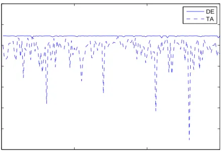
In order to tell which evolutionary approach is more efficient and stable for solving the optimization problem, the fitness values, i.e. the log-likelihood values, from independent restarts of the DE and TA algorithms were compared with each other.
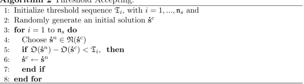
Algorithm 2 Threshold Accepting.
1: Initialize threshold sequenceTi, with i= 1, ...,ns and
2: Randomly generate an initial solution ˙sc
3: fori= 1 to ns do 4: Choose ˙sn∈N(˙sc) 5: if O(˙sn)−O(˙sc)<T i, then 6: ˙sc← ˙sn 7: end if 8: end for
The two algorithms have been restarted 150 times. The fitness values i.e., the log-likelihood values defined in Eq. (8) from restarting the two algorithms, are provided in Figure 1. The figure shows that the DE yields higher and more stable fitness values than that from the TA in each run. The suboptimal performance of the TA is possible due to the simple way used for defining the local neighborhood structure. As Winker [2001] pointed out, the performance of TA highly depends on the construction of local neighborhood structure and the threshold sequence. DE is simpler than TA for implementation as the algorithm only requires a fine tune of the weighting factorK and the crossover probabilityz1. Most of the time,
the solutions from DE are insensitive to small changes of its parameter settings. Due to the above reasons, DE was employed as the EML optimizer in the following simulation study.
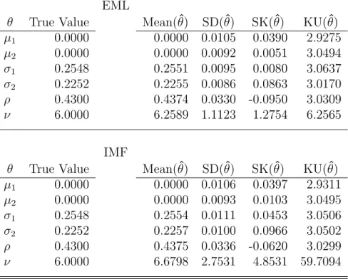
To assess the accuracy of the estimated parameters from the EML estimation against the IFM approach, a set of 200×2 random variables from the bivariate Student t distribution was generated at a total iteration number of nS = 5,000. The true distribution parameters used for generating the random numbers were set as µ1 = 0, µ2 = 0, σ1 = 0.2548, σ2 = 0.2250, ρ = 0.43 and ν = 6. Since the
standard hill-climbing algorithm such as the Newton-Raphson approach for the EML estimation did not generate any results but only for the IFM approach, the results from the IFM were compared with that from the DE procedure applied for the EML estimation. Table 1 shows the numerical results with the standard descriptive statistics of the estimated parameters based on thenS bootstrap
sam-ples. As expected, the EML estimators, obtained by maximizing the log-likelihood function with the DE, are often (i) closer to the true values, (ii) less biased, (iii) less skewed and (iv) less kurtotic as compared to the IFM alternatives.
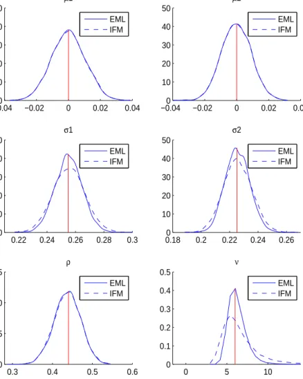
Figure 2 compares the kernel densities of the estimated distribution parame-ters from EML and IFM. As discernible, the differences between the distribution of estimators forµ1, µ2 (top panels) andρ(bottom left panel) are negligible. More
interestingly, the middle panels reveal that the dispersion parameters σ1 and σ2
can be more accurately estimated with the EML approach as their kernel densities are higher in the centered region and lower in the tail regions. Finally, the bottom
0 50 100 150 −1052 −1051.5 −1051 −1050.5 −1050 −1049.5 −1049 −1048.5 Restarts
Maximum log−likelihood values
DE TA
Figure 1: Log-likelihood Value from Independent Restarts
right panel shows that the estimate for the degree of freedom ν that controls the probability of tail events in the distribution is even biased from the IFM method as the peak of its kernel density is not localized at the true parameters position. Overall, it can be seen that the parameters responsible centered moments of the distribution, i.e. σ1, σ2 and ν can be better estimated with the EML approach.
These results are indeed essential as they reveal that the IFM approach often pre-ferred in the financial literature is more likely to provide less reliable estimators of the underlying joint distribution. Hence, the IFM approach based on the gradient search is less able to correctly capture the tail dependence of risk factors (e.g., the extreme losses) than the EML estimation which is powered by the DE algorithm.
Table 1: Comparison of Sample Moments of the Parameters for EML and IFM EML
θ True Value Mean(θˆ) SD(θˆ) SK(θˆ) KU(θˆ)
µ1 0.0000 0.0000 0.0105 0.0390 2.9275 µ2 0.0000 0.0000 0.0092 0.0051 3.0494 σ1 0.2548 0.2551 0.0095 0.0080 3.0637 σ2 0.2252 0.2255 0.0086 0.0863 3.0170 ρ 0.4300 0.4374 0.0330 -0.0950 3.0309 ν 6.0000 6.2589 1.1123 1.2754 6.2565 IMF
θ True Value Mean(θˆ) SD(θˆ) SK(θˆ) KU(θˆ)
µ1 0.0000 0.0000 0.0106 0.0397 2.9311 µ2 0.0000 0.0000 0.0093 0.0103 3.0495 σ1 0.2548 0.2554 0.0111 0.0453 3.0506 σ2 0.2252 0.2257 0.0100 0.0966 3.0502 ρ 0.4300 0.4375 0.0336 -0.0620 3.0299 ν 6.0000 6.6798 2.7531 4.8531 59.7094
−0.040 −0.02 0 0.02 0.04 10 20 30 40 50 µ1 EML IFM −0.040 −0.02 0 0.02 0.04 10 20 30 40 50 µ2 EML IFM 0.22 0.24 0.26 0.28 0.3 0 10 20 30 40 50 σ1 EML IFM 0.180 0.2 0.22 0.24 0.26 10 20 30 40 50 σ2 EML IFM 0.3 0.4 0.5 0.6 0 5 10 15 ρ EML IFM 0 5 10 0 0.1 0.2 0.3 0.4 0.5 ν EML IFM
5
Comments and Summary
This paper suggests implementing an evolutionary algorithm in the exact maxi-mum likelihood estimation of a multivariate Student t copula model. Usually, the standard Newton-Raphson algorithm fails to solve complex optimization prob-lems such as the EML estimation for the parameter inference of copula models, while a derivative-free optimizer can conquer such problems. Two evolutionary ap-proaches, namely Differential Evolution and Threshold Accepting were employed to tackle the EML estimation problem, and it has been found that the former yielded a better performance. Through a simple simulation study, it has been proven that the proposed methodology for EML estimation already provided rea-sonably good results in a simple two-dimensional setting with a Student t copula model. As it is expected, the estimates obtained by the EML approach enhanced with Differential Evolution are often closer to the true values as compared to the IFM alternatives. Differential Evolution should be competent for the EML in-ference of more complicated copula models than the bivariate Student t copula studied in this paper.
References
Bollerslev, T. (1987). A conditional heteroskedastic time series model for specula-tive prices and rates of return. Review of Economics and Statistics, 69:542–547. Dueck, G. and Scheuer, T. (1990). Threshold Accepting: A general purpose op-timization algorithm appearing superior to simulated annealing. Journal of Computational Physics, 90:161–175.
Fantazzini, D. (2009). Three–stage semi–parametric estimation of t-copulas: Asymptotics, finite-sample properties and computational aspects. Computa-tional Statistics and Data Analysis, doi:10.1016/j.csda.2009.02.004.
Joe, H. (1997). Multivariate Models and Dependence Concepts. Chapman & Hall, London.
McNeil, A. J., Frey, R., and Embrechts, P. (2005). Quantitative Risk Management. Princeton University Press, New Jersey.
Meucci, A. (2005). Risk and Asset Allocation. Springer, Berlin. Nelsen, R. B. (1998). An Introduction to Copulas. Springer, Berlin.
Price, K., Storn, R., and Lampinen, J. (1998). Differential Evolution: A practical approach to global optimization. Springer, Berlin.
Sklar, A. (1959). Fonctions de r´epartition `a n dimensions et leurs marges. Publi-cations de 1’institut de statistique de 1’Universit´e de Paris, 8:229–231.
Storn, R. and Price, K. (1997). Differential Evolution – A simple and efficient heuristic for global optimization over continuous spaces. Journal of Global Op-timization, 11:341–359.
Winker, P. (2001). Optimization Heuristics in Econometrics: Applications of threshold accepting. John Wiley & Sons, West Sussex.
Zhang, J. and Ng, W. L. (2010). EML–estimation of multivariate t copulas with heuristic optimization. In Proceedings of International Conference on Computer Science and Information Technology, pages 469–473.