Effective Matrix Factorization for Online Rating Prediction
Bowen ZhouComputer Science and Engineering University of New South Wales Kensington, NSW, Australia 2052
Raymond K. Wong Computer Science and Engineering
University of New South Wales Kensington, NSW, Australia 2052
Abstract
Recommender systems have been widely utilized by online merchants and online advertisers to promote their products in order to improve profits. By evaluating customer interests based on their purchase history and relating it to commodities for sale these retailers could excavate out products which are most likely to be cho-sen by a specific customer. In this case, online ratings given by customers are of great interest as they could reflect different levels of customers’ interest on differ-ent products. Collaborative Filtering (CF) approach is chosen by a large amount of web-based retailers for their recommender systems because CF operates on interactions between customers and products. In this paper, a major approach of CF, Matrix Factorization, is modified to give more accurate recommendations by predicting online ratings.
1. Introduction
Most online retailers provide the public, who have different interests, with a great variety of products and services. Therefore, in order to cater for customers interests by helping them in making choices from the large number of various items, recommender systems are increasingly used to shrink the range of products that might be attractive to a specific customer.
Based on accurate recommendations, sellers could gain their reputation among customers and increase the possibility that users make a purchase on recommended products. It has been shown by other researchers that movie recommender systems could be used to maxi-mize revenues by applying effective algorithms [1].
Recommender systems usually take into considera-tion profiles of users and items respectively and give recommendations by applying algorithms on the in-formation of attributes and/or users purchase history retrieved from these profiles and evaluating users
po-tential preferences of each item. There are two main approaches that could be used for the purpose of rec-ommending products effectively. One is called Content-Based filtering, which creates a profile describing the types of items the user is interested in and a profile containing descriptions of items, and generates recom-mendations based on these two profiles [2].
Another approach called Collaborative Filtering gen-erates recommendations based on users behaviour [3]. This approach focuses on a group of users or items that have similar behaviour or attributes and establishes relationships between each user (user-based filtering) or each item (item-based filtering) by analysing responds (e.g. movie ratings) each user gives to each item. In this case, responses from users to items are not only restricted to what users prefer, implicit feedbacks such as what users dislike are also of great significance [4]. One of CF approaches, Matrix Factorization (MF), has been popular in recent years. Most MF researches improve the accuracy by taking the data (e.g. movie ratings) as the point of penetration without considering the impact of item attributes [5], [6], [7]. Although these new MF approaches can provide more accurate ratings, an improvement from different perspective will be necessary when they reach a bottleneck.
Also, a qualified MF-based approach developed by Koren in [8] shows a problem of extreme long training time. His approach provides precise predictions for movie ratings while runs for 17 minutes for each iteration when there are 50 factors. In this case, if the practical recommender system updates the models frequently after receiving feedbacks from users and the number of active users is high, the server might suffer from the operation time.
Another trouble most CF approaches (not only MF) face is the cold-start problem. If a user has only few historic data available to the recommender system, it would be difficult to generate accurate recommen-dations or give accurate predictions to this user. A free software called MyMediaLite, developed by Zeno, Proceedings of the 50th Hawaii International Conference on System Sciences | 2017
Steffen, Christoph and Lars [9], gives predictions to new users by simply returning the global average of all the ratings. More precisely, authors of [10] provides a way to reduce the prediction error a little for those who have rated for few items.
To address these issues, this paper firstly takes attributes into consideration to enhance the accuracy of the original MF approach. Then the theory of k-nearest-neighbour approach will be implemented along with the improved MF approach to give more accurate predictions. Also, an effective method is used deal with cold-start problem and the effect is compared with [10]. In summary, the contributions of this paper can be summarized as follows:
• Item attributes are taken into consideration to enhance the accuracy of the MF approach; • Ratings ofknearest neighbours of predicted items
are used to modify the predictions for more accu-rate recommendation;
• An improved MF approach mines the most signif-icant data to deal with cold-start problem. The rest of this paper is organized as follows. Section 2 summarizes related work in Content-Based recommendations, Collaborative Filtering and Matrix Factorization (MF) based approaches. Details of MF are provided in Section 3. After that, we present our MF based approach in Section 4. Section 5 describes the experiments that show the effectiveness of our approach and Section 6 discusses the result. Finally, Section 7 concludes the paper.
2. Related work
Many recommendation methods have been studied due to the great demand in the current age of big data. Recommendation approaches are split into two types: Content-Based (CB) and Collaborative Filtering (CF).
2.1. Content-Based Recommendation
CB consists of three steps: Information Retrieval, Profile Learning, and Recommendation Generation. 2.1.1. Information Retrieval: In real applications the attributes of items can be distinguished as structured or unstructured information, as stated in [2]. Structured attributes often have explicit meaning and the values are within a certain range (e.g. age, gender), while unstructured attributes are often implicit and there are no restrictive range for their values (e.g. purchase his-tory). Different from structured attributes which can be directly used in recommendation systems, unstructured information needs to be extracted from a fragment of contents in order to be quantized. An example of Vector
Space Model (VSM) is given in [2], which is the most commonly used approach to retrieve information from a section of text.
2.1.2. Profile Learning: This step is to build a model for a user according to his preference in the past. Based on this model, recommendation systems can infer whether this user will like/dislike a new item. This step can be basically considered as a supervised classification learning step. A typical profile learning approach in CB is the k-nearest-neighbour approach (KNN) which evaluates most similar items according to their attributes. Naive Bayes (NB) is also com-monly implemented for profile learning, particularly for document classification. By calculating posterior probabilities, NB will assign an item to one of the two classes: user likes or user dislikes.
2.1.3. Recommendation Generation: This step sim-ply returns the top-N items which attracts user the most according to results in profile learning.
2.2. Collaborative Filtering
There are two main types of CF: memory-based CF (user-based and item-based) and model-based CF [11]. Examples of memory-based CF approaches are given in [12], [13]. Memory-based CF finds nearest neighbours of a user by searching through the entire user database and generates a list of recommended items. Ka, Anto, Volker, Xiaowei and Hans-Peter de-veloped their probabilistic memory-based CF approach and they stated that the approach needs to scan the whole database to construct the profile space of users [14]. In order to deal with the computation complexity and memory bottleneck problem, theirshift of workload provides an efficient way, in which construction of the profile space can be considered as a backstage operation and will be conducted only when there is available computing power. Also, in order to deal with the long computation time, an item-based CF, which can obviously shorten the operation time without negatively affecting accuracy of prediction, is provided in [15].
Model-based CF uses user database to build a model to store ratings, which could alleviate scalability and sparsity issues [10]. Although model-based CF can provide predictions of similar quality to memory-based CF, it often takes long time to build and train the offline model, and it is difficult to update models. There are some commonly implemented model-based CF such as clustering algorithm, singular value de-composition (SVD), and Bayesian network. Clustering algorithm treats recommendation as a classification problem, which means that it iteratively computes the center of clusters and classify which cluster a user
should be assigned into based on the distance learning approach, and then give recommendation according to components in nearest clusters [10], [16]. SVD is closely related to the Matrix Factorization method that will be discussed later in this paper. It decomposes the original rating matrixRbyA=U×S×VT, whereU andV are the left and right singular vectors and S is the diagonal matrix, and then chose the first k singular values to reduce the dimension of the diagonal matrix S. The reconstruction of Rk = Uk ×Sk ×VkT gives therank-kmatrix which is the closest approximation of the original rating matrix [17]. Also, SVD is commonly used together with principal component analysis (PCA) to reduce the dimension of the original database [10], [18]. Bayesian network model, which is also called probabilistic directed acyclic graphical model, operates with conditional probability. In the network, probability of a variable influencing others is evaluated and then recommendation will be given based on dependencies between pairs of variables [11], [19], [20].
2.3. Matrix Factorization
There are some other researchers who improved the MF approach for more accurate predictions. Yifan, Yehuda and Chris introduced a model with probability and confidence to obtain more accurate values of user factors and item factors [5]. Hanhuai and Arindam used a Gaussian prior with an arbitrary mean over u and
v, and combined the correlated topic model and latent Dirichlet allocation work with their matrix model [6]. Vikas, Serhat, Jianying and Aleksandra introduced a new binary matrix, in which 0 means ‘not purchased’ and 1 means ‘purchased’, into the factor-learning pro-cess in non-negative Matrix Factorization (NMF) ap-proach [7]. Compared to the above algorithms, the pro-posed new MF approach in this paper concentrates on transforming the original rating matrix and modifying already-predicted ratings using item attributes. It might be possible to combine the proposed MF with previous approaches to give more accurate predictions since it achieves improvement from different perspective.
The k-nearest-neighbour (KNN) approach (different from KNN in Content-Based approaches) which eval-uates neighbours based on ratings given by users, has been studied to be applied in recommender systems [21], [22]. Compared to the classic KNN technique, Matrix Factorization (MF) method proved to be more accurate when it is used to deal with datasets such as the one provided by the online DVD rental company Netflix, as stated by the winner of Netflix prize [23], so it has become a dominant approach of Collaborative Filtering recommenders and is decided to lead to the
solutions to MovieLens dataset in this paper.
3. Matrix factorization with stochastic
gradient descent
MF is basically based on matrixRcontaining ratings given by a userui to an itemvj. The total number of users and items isM andN respectively.
3.1. Matrix factorization
R= r1,1 · · · r1,j · · · r1,n : . .. : . .. : ri,1 · · · ri,j · · · ri,n : . .. : . .. : ri,1 · · · ri,j · · · ri,n R= r1,1 · · · ? · · · ? : . .. : . .. : ? · · · ri,j · · · ? : . .. : . .. : ? · · · ri,j · · · ri,n As shown by the first M ×N matrix, each entity, denoted byri,j, in the matrix refers to a rating userui gives to the item vj, and the second matrix demon-strates that in most cases a majority of ratings are not available and need to be predicted. Therefore, the aim of MF algorithm is to predict all of the unknown ratings. LetU denote aM ×K matrix and V denote aN×K matrix respectively, whereK is the number of factors which need to be iteratively learned by the MF algorithm to generate a matrix such that R ≈Rˆ, meaning that each entity in Rˆ represents a prediction of a rating. In this case, a specific rating ri,j can be evaluated by calculating the dot product of relevant rows inUandV respectively. Letuidenote thei-throw ofU andvidenote thei-throw ofV, and the predicted rating ri,j can be simply obtained via Equation (1).
ˆ
ui,k andvj,kˆ in the equation are the approximation of the factors of users and items, which are not given, so they need to be learned by recommender systems to implement this formula.
ˆ ri,j= K X k=1 ui,k×vj,k= K X k=1 ˆ ui,k×vˆj,k=ui·vTj (1)
3.2. Stochastic Gradient Descent
A problem of Equation (1) is that factors of users and items are undiscovered so that they need to be learned
by minimizing prediction errors obtained through the training set Twhich contains given ratings (2).
erri,j= ˆri,j−ri,j ∀ri,j∈T (2) First of all, normal distribution is used to initialize factors in U and V. It is too restrictive to require only local minimization for some problems including [24], so stochastic gradient descent (SGD) algorithm, which iteratively modifies parameters to converge to a stationary point after some number of iterations [25], is chosen to be implemented iteratively through the training dataset to find the best-fit factors. Throughout SGD, each user factor will be updated as shown in (3), where η is the learning rate/step size (usually set to less than 0.2) and E is the error denoted by squared error 12( ˆri,j−ri,j)2 so that ui,k will be increased by the gradient of E with respect to ui,k itself. Equation (4) shows the update for item factorvj,k.
ui,k=ui,k+η ∂E ∂ui,k (3) vj,k=vj,k+η ∂E ∂vj,k (4) By further calculation, the partial differential com-ponents in (3) and (4) can be simplified into (5) and (6), wherenis the number of factors
∂E ∂ui,k = ∂ 1 2( ˆri,j−ri,j) 2 ∂ui,k
= ( ˆri,j−ri,j)·∂rˆi,j
∂ui,k = ( ˆri,j−ri,j) ∂(ui,1vj,1+· · ·+ui,nvj,n) ∂ui,k = ( ˆri,j−ri,j)·vj,k (5) ∂E ∂vj,k
= ( ˆri,j−ri,j)·ui,k (6) Below is the pseudo code for SGD algorithm used for MF. All the ratings in the training set R are sorted in random order, and within each iteration the randomly ordered rating will be used in sequence to implement (5) and (6). After iterating for numIter times, only factors related to given ratings will be updated to give the minimum error. For example, ifr5,7is not given in
R, u5,1···numF actors andv7,1···numF actors will remain the same value as generated by normal distribution at the start of SGD procedure.
Input: training set R, number of factors numFactors, number of iteration numIter Output:U andV with learned entities (factors) Forn= 1 :numIter
For each ratingri,j inR, in random order For each factorui,k, vj,k∈[1, numF actors] ui,k =ui,k+ηu∂E
i,k,vj,k=vj,k+η ∂E vj,k
3.2.1. Overfitting: Since in the learning procedure the update of each user factor is only affected by item factor, and the item factor is changed only according to user factor, there exists a possibility that the learned factors are overfitting the training dataset, as illustrated in Figure 1. So a regularization process is introduced, which substitutes the user factors into the update of user factors, and the action for item factors is the same, as shown in euqation (7).λis the regularization coefficient and there is no need to find a precise value of it because it is only used to preventui,k from “over oscillating”.
Figure 1:ui,k goes away from the stationary point from
step 2 to step 3 ui,k=ui,k+η( ∂E ∂ui,k −λ·ui,k) (7)
4. Proposed Approaches
In this section, the proposed approaches will be discussed in detail.
4.1. MFA: Inserting movie attributes into
dataset
Suppose that each movie has h manually defined attributes, so these attributes could be utilized to revise item factors. Firstlyhvirtual users will be created, and for each of virtual users, a spurious rating of each movie, the value of which would whether be min and max, will be assigned according to whether this specific movie has this specific attribute or not, where min andmaxare the minimum and maximum rating values defined in the dataset. For example, if the10th movie has the 5th attribute, max will be assigned to the virtual rating given by the(numU sers+ 5)th to the 10thmovie, and if the 11th movie does not have the 5th attribute, min will be assigned to the virtual rating given by the (numU sers+ 5)th to the 10th movie, wherenumU sersis the total number of users existing in the dataset. In this case, when SGD operates on the newly inserted virtual ratings, item factors of corresponding movies in V will be modified and the predicted rating rˆi,j will then be affected. The theory behind is that if two movies A and B have similar
attributes (e.g. both of them are romantic movies), during SGD item factors of A and B will similarly be increased or decreased, and this leads to the fact that item factors would be altered not only according to interactions between users and movies, but also in accordance with relationship between movies. In this stage, the proposed approach is named MFA.
4.2. MFA KNN: Combine MF with K nearest
neighbour
The k-nearest-neighbour method concentrates on the relationship between pairs of items, and then give recommendation based on the similarity between items. For example, if a user gives full mark to movieA, and movieBhas a high similarity withA, the recommender system will generate a result that this user will enjoy B. Also, similar users might give close ratings to a specific movie. Different from the similarity estima-tion described in Secestima-tion 2.2, the relaestima-tionship between items can be evaluated by distance learning, as shown in Equation (8). Disp(x,y) is called the MinKowski
distance, and x and y are the attribute vectors of item x and item y respectively. The most commonly used “distance” areManhattan distanceandEuclidean distance, which setpto 1 and 2 respectively.
Disp(x,y) = ( d X j=1 |xj−yj|p) 1 p =||x−y||p (8)
If two movies m1 and m2 both have h attributes,
then m1 and m2 can be respectively denoted by m1
and m2, each of which is a vector with h elements. Applying the above theory will give Equation (9).
Disp(m1,m2) = ( h X j=1 |m1,j−m2,j|p) 1 p =||m1−m2||p (9)
Theoretically, if some of the nearest neighbours of an itemv to be predicted for a user have already been rated by him/her, the accuracy of prediction of v can be improved by the difference between its neighbours’ ratings and the average rating. This will be proved in the experiment. Also, it needs to be noticed that com-bining KNN with MF will not influence item factors so that it can be combined with other CF approaches.
4.3. Bias in prediction
Equation (1) simply takes the summation of product of each user factor and each item factor. It focuses on interactions between users and items but ignores the effects caused by users themselves. For example,
some users with rigorous critical thinking prefer to give lower ratings to each movie than the public, while some lenient users always give inspiring ratings (e.g. over 4 out of 5) to all of the movies. A bias is introduced to classify users of different tolerance.
ˆ ri,j= ¯ri+ K X k=1 ˆ ui,k×vˆj,k= ¯ri+ui·vTj (10) ˆ ri,j= ¯r+ K X k=1 ˆ ui,k×vˆj,k= ¯r+ui·vTj (11)
Equation (10) introduces a biasr¯i into the original
evaluation of predicted ratings in Equation (1). In this case, predictions of users who tend to give low/high ratings will be lowered/increased by the factorr¯i, which
is the average rating of useri, regardless of user factors and item factors obtained through SGD. Also, the increment, ∂u∂E
i,k, will not change due to the property
of partial derivatives. Similarly, Equation (11) uses the global mean¯ras the bias, which can possibly avoid the problem caused by lack of ratings of some particular users who have rated only digital number of movies. The accuracy of these two biases needs to be tested.
4.4. MFAR: Setting threshold for cold-start
problem
As most other Collaborative Filtering approaches [27], cold-start is a common problem for MF. It means that if a user has rated only few movies, recommender systems might not give predictions accurately due to lack of information of this user. To deal with this problem, a thresholdthwill be used to filter out most misleading ratings, meaning that ratings whose pre-diction error exceeds the threshold will be considered to negatively affect the accuracy of prediction. If a rating given by a cold-start user to movie is filtered out, it means that this rating is considered to mislead the user factors of this cold-start user, and if a rating of a movie which is not given by a cold-start user is filtered out, this rating is considered to mislead the item factors of this movie. More specifically, during SGD, after some number of iterations, if the absolute error of the prediction of an instance (ratings or attributes) in training dataset is still greater thanth, this instance will not be used in the prediction.
5. Experiment
5.1. Parameter setting for MF
In this experiment, a dataset provided by Movielens is used. This dataset consists of 100,000 instances of
form (i, j, ri,j), where i and j represent user ID and
item (movie) ID respectively, and each instance refers to a rating ranging from1to5given by a specific user out of 943 to a specific movie out of 1682, so that the sparsity of this dataset is 1− 100000
943×1682 = 93.7%.
The first part of the experiment will be testing how the accuracy of MF will be affected by two dominant parameters, number of iterations and number of factors. The test will be implemented usingall but n method, in whichn ratings of each user will be extracted as a testing dataset, and the remaining data will be used as the training set. The number of extracted ratingsnis set to5,10,15, and20respectively. Additionally, running time with respect to different parameter values will be measured to obtain a trade-off between algorithms complexity and accuracy. In order to show results, root mean square error (RMSE) and mean absolute error (MAE) will be used to illustrate how the predicted rat-ings differ from the true value. During the experiments, the parameter not to be tested will be fixed when the measurement is to be taken for the other.
RM SE= s
P
i,j( ˆri,j−ri,j)2 N
M AE = P
i,j|rˆi,j−ri,j| N
5.2. MF with movie attributes
In order to improve the accuracy of the tradi-tional MF approach, attributes of movies will be inserted into the original dataset. 19 attributes of movies are provided by MovieLens of the form
(movieID, a1, a2· · ·ai· · ·a19), where ai = 0 if this
movie does not have thei-thattribute andai= 1 other-wise. The new MFA approach will treat each attribute as a new user, as shown below. Theoretically, MFA will learn factors more accurately due to similarity and difference among 1682 movies, with the premise that the number of newly inserted attributes are not much larger than the number of ratings, otherwise the overfitting problem might be caused.
Input: 19 attributes of 1682 movies, DatabaseD
Output: New database D with movie attributes For each moviem
For each attributeam,i of m
Ifam,i= 0, Insert(943 +am,i, m,1) intoD
Ifam,i= 1, Insert(943 +am,i, m,5) intoD
5.3. Bias
In previous sections, the global mean of the entire training dataset is used as the bias in the SGD and prediction generation process. In order to show the influence of using each user’s average rating to learn factors and give predictions, a test will be taken for 1000 times and t-test will be used to show whether the accuracy of these two settings differ. In this section, 5 ratings of each user will be extracted out as the test data, and the remaining will be the training data. The reason is that some users in the Movielens dataset have rated for only 20 movies, so that if too many ratings of these users are extracted it will be harder to explain the prediction evaluated based on their average ratings.
5.4. Combine MF with KNN
The KNN approach findsk neighbours of an object by calculating the similarity between all of the other objects with it. For example, the traditional KNN approach takes an average of the values of an objects
k nearest neighbours to give a prediction. A more accurate KNN approach has been shown by another researcher in [28]. This part will modify each predicted ratingri,jbyknearest movies of movievj which have been rated by userui, as illustrated in Equation (12).
ˆ
ri,j= ˆri,j+σ·
X
(ri,n−r¯i) ∀n∈KN N(j) (12)
KNN of a movie will be determined by the distances between it and other movies. The calculation of dis-tance is shown in Equation (13), where ai andbi are
the attribute vectors of movieA andB respectively.
dist(A, B) =X
i
|ai−bi| (13) The theory behind is that if the similarity between movieA andB is relatively high, the prediction ofB
given by a user should be affected by the true rating of A if the same user has rated for it. The factor
(ri,n −ri¯), which represents the user preference of movien, is negative if the users rating for n is below his/her average rating and is positive in another case. Value of σ should be carefully chosen, otherwise the modification would increase error of the prediction.
5.5. MFAR for cold-start problem
As most other Collaborative Filtering approaches [27], cold-start is a difficult but common problem for MF. It means that if a user has rated only few movies, recommender systems might not give predictions ac-curately due to lack of information of this user. To deal with this problem, a threshold t will be used to
filter out most useless data, meaning that data whose prediction error exceeds the threshold will be consid-ered to negatively affect the accuracy of prediction. More specifically, during SGD, after some number of iterations, if the absolute error of the prediction of an instance (ratings or attributes) in training dataset is still
greater than t, this instance will not be used in the
prediction. In this part, 500 users will be randomly chosen, and 300 of them will be placed in the training
set, andnratings of each of the left 200 users will also
be inserted into the training set. The remaining ratings of these 200 users will be used as the testing set. This
approach is named as Given n, wherenis set to 5, 10,
15, and 20 respectively. This test method was also used in other researches including [10] and [29]. In all of the above experiments, tests will be operated 10 times in each case to give an average to avoid ‘extreme’ values.
5.6. Testing platform and device
Different from Hadoop, one of the distributed frame-works, which utilized HDFS to split large data file into several blocks with some replications to store them in different data-nodes (storage part) and uses MapReduce to process the data in parallel, this paper only focuses on single machine. During the experiment, the program is run on OS X EI Capitan. The machine used is Macbook with a 2.0 GHz quad-core Intel Core i7 processor (Turbo Boost up to 3.2 GHz) with 6 MB shared L3 cache. Memory is 8 GB of 1600 MHz DDR3L, and the machine has 256 GB flash storage.
6. Results and discussion
6.1. Number of iterations
Figure 2: Matrix Factorization performance with respect to number of iterations
The number of iterations is the first parameter tested to show the relationship with the recommendation quality. It is assigned from 10 to 100 with an increment of 10, and the test is based on the traditional MF approach. Figure 2 indicates that for all the number of ratings to be predicted (e.g. 5 to 20 with an increment
of 5), prediction error of MF keeps decreasing while number of iterations increases and it converges to a stationary point when number of iterations reaches 50. The operation time of MF has a steady growth rate
during the rise of this parameter. Therefore,numIter
is set to 50 for the following experiments.
Figure 3: Matrix Factorization performance with respect to number of factors
Similarly, as illustrated in Figure 3, the accuracy of MF rises with the increase of number of factors, and running time is approximately proportional to it.
According to this result,numF actorsis set to 5 for the
following improved MF approaches. The above results
show that the running time for differentnvalues with
the same parameter settings does not vary too much. It is because that the data in training set dominates the complexity of MF. If only 20100000×943 = 18.86% ratings are used as testing data, and the remaining data are used to learn factors iteratively (e.g. 50 times), there
is no doubt that n value will only have insignificant
influence on the operation time.
6.2. MF with movie attributes MFA & use of
KNN
Figure 4: Mean absolute error of improved Matrix Factorization approaches
After inserting attributes of movies into the training set, the prediction is supposed to be more accurate, and Figure 4 and Figure 5 display the prediction error before and after using attributes, where MF is the traditional Matrix Factorization method and MFA is the method using attributes. In all of the 4 cases where the number of data extracted for each user varies from 5
Figure 5: Root mean square error of improved Matrix Factorization approaches
Table I: t-test for KNN
t-Test: Two-Sample Assuming Unequal Variances
MF MF with KNN Mean 0.762332362 0.760927889 Variance 0.000135418 0.000139141 Observations 1000 1000 Hypothesized Mean Difference
0 (test whether two samples are equal)
t Stat 2.680376141
t Critical two-tail 1.961152015
to 20, MFA always gives better prediction than MF. In addition, K = 10 and = 0.06 are the configurations for combining MF and MFA with KNN method, which use a specific movies most similar movies to modify pre-dicted ratings. The figures indicate that the prediction error decrease by a small number when KNN is used for further modification. Table I shows the results of t-test which takes 1000 samples of MF and MF with KNN respectively. With a confidence level of 95%, t value (2.680376141) is greater than the critical t value (1.961152015), which means that the prediction error of MF ‘really’ exceeds the error of MF with KNN. It provides an evidence that the similarity of items will similarly attract a user to some extent.
6.3. Bias
In order to show whether biases in Equation (10) and (11) have different impacts on the accuracy, 1000 samples were used to perform t-test. With a confidence level of 95%, as shown in TABLE II, t value of the difference in two mean values is less than the negative critical t value (-1.9612), which means that
Table II: t-test for bias
t-Test: Two-Sample Assuming Unequal Variances MF user mean in SGD MF global mean in SGD Mean 0.755682927 0.762332362 Variance 0.000134362 0.000135418 Observations 1000 1000 Hypothesized Mean Difference
0 (test whether two samples are equal)
t Stat -12.80206157
t Critical two-tail 1.961152015
using each user’ mean rating in SGD and prediction generation can “really” improve the accuracy. However, one shortcoming of using each user mean is that when the test was performed for all but 20 and all but 15, the result was not as satisfactory as using global mean. So, due to the poor stability, whether user mean or global mean should be used needs to be carefully decided.
6.4. MFAR for cold-start problem
Figure 6: Impact of different values of threshold
Figure 7: Matrix Factorization approaches dealing with cold-start problem, shown in MAE
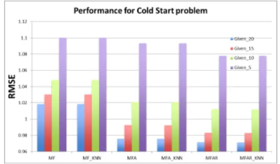
Figure 8: Matrix Factorization approaches dealing with cold-start problem, shown in RMSE
Firstly, in order to learn the influence of different threshold on prediction accuracy, the number of given ratings of each user is set to 5. During the test, threshold varies from 0.1 to 2.9 with an increment of 0.1, and the experiment is averaged over 10 iterations. As shown in Figure 6, MAE drops dramatically at the beginning and reaches the minimum value when threshold is between
Table III: Comparison with others’ approaches
Approach all but 10 training 80%
MFA with KNN 0.7560981 0.748411
PCA-GAKM [10] 0.7821 –
Pearson Correlation Similarity [18] – 0.828 Euclidean Distance Similarity [18] – 0.818
Log Likelihood [18] – 0.817
Tanimoto Similarity [18] – 0.794
Table IV: Comparison with others’ approaches for cold-start problem
Given 5 Given 10 Given 15 Given 20
MFAR 0.8485 0.7961 0.7743 0.7663
[10] approx. 0.90 0.82 0.79 0.77
1.5 and 2.0. The reason is that when threshold has small value (e.g. 0.1 to 1.0), most of the ratings in training dataset will be considered asmisleading, and consequently there will not be enough training data to accurately learn the compulsory factors. Additionally, when threshold reaches large value (e.g. larger than 2.5), more misleading ratings will not be filtered out because the prediction error of these ratings will not ex-ceed the threshold. Therefore, compared to the number of ratings of each user provided (i.e. 5), large amount of movie attributes will mislead the factors learned by SGD. According to the result shown in Figure 6, the threshold is set to 1.7 in the following experiments.
When MF is used to deal with cold-start problems, the number of given ratings of each user is set to 5, 10, 15, and 20 respectively. As shown by Figure 7 and Figure 8, combination of MF and KNN fails to make contributions to the accuracy of prediction, which might be because that the extreme small number of given ratings in training set fail to provide nearest neighbours of predicted movies. For Given 20, Given 15, and Given 10, MAE of MF, MFA and MFAR decrease progressively, but for Given 5, MAE of MF and MFA is almost the same. RMSE has a similar trend, with MFAR providing the most accurate prediction.
6.5. Comparison with others’ algorithm
It is convenient to compare the proposed MF algo-rithm with other researchers’ approaches such as [10] and [18], as they also used the the Movielens 100K dataset and showed their results in RMSE and MAE.
As shown in Table III, authors of [10] provided the precise value of their PCA-GAKM method forall but 10 test, and in comparison, the proposed MFA-KNN method has better performance. Dheeraj, Sheetal and Debajuoti measured their algorithms under the condi-tion that the ratio of training set and testing set was 80%:20% [18], and MFA-KNN also has more qualified prediction quality. Table IV compares the accuracy of MFAR with PCA-GAKM. MFAR always has more
accurate prediction than PCA-GAKM regardless of the number of ratings provided by each user.
7. Conclusion
In this paper improved Matrix Factorization methods are developed to give more accurate predictions. The traditional MF approach is firstly studied to show its performance with respect to number of iterations and number of factors. Attributes of movies are then inserted into the training set in order to help the algorithm in learning factors, and the results show that the insertion can obviously increase accuracy of rating prediction. Also, since similar movies might have close attractiveness to users, k-nearest-neighbour approach is implemented to further improve the prediction, and the experiment supports this hypothesis. Finally, to deal with cold-start problem, which is one of the most com-mon problems for Collaborative Filtering, a reduction approach is used to filter out the most useless in the training set. The carefully selected threshold t proved to effectively reduce the prediction error for those who have insufficient ratings (5-20 during the experiment). Our ongoing work includes adjustments (or exten-sions, if needed) to our proposed method to make it generic for a variety of prediction applications. We are also interested in combining our method with other work on non-negative Matrix Factorization to achieve more accurate predictions.
References
[1] A. Azaria, A. Hassidim, S. Kraus, A. Eshkol, O. Wein-traub, and I. Netanely, “Movie recommender system for profit maximization,” in Proceedings of the 7th ACM conference on Recommender systems. ACM, 2013, pp. 121–128.
[2] M. J. Pazzani and D. Billsus, “Content-based recom-mendation systems,” inThe adaptive web. Springer, 2007, pp. 325–341.
[3] D. Bokde, S. Girase, and D. Mukhopadhyay, “Matrix factorization model in collaborative filtering algorithms: A survey,” 2015.
[4] P. Melville, R. J. Mooney, and R. Nagarajan, “Content-boosted collaborative filtering for improved recommen-dations,” inAAAI/IAAI, 2002, pp. 187–192.
[5] Y. Hu, Y. Koren, and C. Volinsky, “Collaborative fil-tering for implicit feedback datasets,” inData Mining, 2008. ICDM’08. Eighth IEEE International Conference on. Ieee, 2008, pp. 263–272.
[6] H. Shan and A. Banerjee, “Generalized probabilistic matrix factorizations for collaborative filtering,” inData Mining (ICDM), 2010 IEEE 10th International Confer-ence on. IEEE, 2010, pp. 1025–1030.
[7] V. Sindhwani, S. S. Bucak, J. Hu, and A. Mojsilovic, “One-class matrix completion with low-density factor-izations,” in Data Mining (ICDM), 2010 IEEE 10th International Conference on. IEEE, 2010, pp. 1055– 1060.
[8] Y. Koren, “Factorization meets the neighborhood: a mul-tifaceted collaborative filtering model,” inProceedings of the 14th ACM SIGKDD international conference on Knowledge discovery and data mining. ACM, 2008, pp. 426–434.
[9] Z. Gantner, S. Rendle, C. Freudenthaler, and L. Schmidt-Thieme, “Mymedialite: A free recommender system library,” in Proceedings of the fifth ACM conference on Recommender systems. ACM, 2011, pp. 305–308.
[10] Z. Wang, X. Yu, N. Feng, and Z. Wang, “An improved collaborative movie recommendation system using com-putational intelligence,”Journal of Visual Languages & Computing, vol. 25, no. 6, pp. 667–675, 2014. [11] J. S. Breese, D. Heckerman, and C. Kadie, “Empirical
analysis of predictive algorithms for collaborative fil-tering,” inProceedings of the Fourteenth conference on Uncertainty in artificial intelligence. Morgan Kauf-mann Publishers Inc., 1998, pp. 43–52.
[12] J. Wang, A. P. De Vries, and M. J. Reinders, “Uni-fying user-based and item-based collaborative filtering approaches by similarity fusion,” in Proceedings of the 29th annual international ACM SIGIR conference on Research and development in information retrieval. ACM, 2006, pp. 501–508.
[13] H. J. Ahn, “A new similarity measure for collaborative filtering to alleviate the new user cold-starting problem,” Information Sciences, vol. 178, no. 1, pp. 37–51, 2008. [14] K. Yu, A. Schwaighofer, V. Tresp, X. Xu, and H.-P. Kriegel, “Probabilistic memory-based collaborative fil-tering,”Knowledge and Data Engineering, IEEE Trans-actions on, vol. 16, no. 1, pp. 56–69, 2004.
[15] B. Sarwar, G. Karypis, J. Konstan, and J. Riedl, “Item-based collaborative filtering recommendation al-gorithms,” in Proceedings of the 10th international conference on World Wide Web. ACM, 2001, pp. 285– 295.
[16] L. H. Ungar and D. P. Foster, “Clustering methods for collaborative filtering,” in AAAI workshop on recom-mendation systems, vol. 1, 1998, pp. 114–129. [17] B. Sarwar, G. Karypis, J. Konstan, and J. Riedl,
“In-cremental singular value decomposition algorithms for highly scalable recommender systems,” in Fifth In-ternational Conference on Computer and Information Science. Citeseer, 2002, pp. 27–28.
[18] D. kumar Bokde, S. Girase, and D. Mukhopadhyay, “An item-based collaborative filtering using dimensionality reduction techniques on mahout framework,” CoRR, 2015.
[19] T. D. Nielsen and F. V. Jensen,Bayesian networks and decision graphs. Springer Science & Business Media, 2009.
[20] C. Ono, M. Kurokawa, Y. Motomura, and H. Asoh, “A context-aware movie preference model using a bayesian network for recommendation and promotion,” in User Modeling 2007. Springer, 2007, pp. 247–257. [21] T. Hong and D. Tsamis, “Use of knn for the netflix
prize,”CS229 Projects, 2006.
[22] P. G. Campos, A. Bellog´ın, F. D´ıez, and J. E. Chavar-riaga, “Simple time-biased knn-based recommenda-tions,” in Proceedings of the Workshop on Context-Aware Movie Recommendation. ACM, 2010, pp. 20– 23.
[23] Y. Koren, R. Bell, and C. Volinsky, “Matrix factorization techniques for recommender systems,”Computer, no. 8, pp. 30–37, 2009.
[24] T. S. Ferguson, “An inconsistent maximum likelihood estimate,”Journal of the American Statistical Associa-tion, vol. 77, no. 380, pp. 831–834, 1982.
[25] R. Gemulla, E. Nijkamp, P. J. Haas, and Y. Sisma-nis, “Large-scale matrix factorization with distributed stochastic gradient descent,” inProceedings of the 17th ACM SIGKDD international conference on Knowledge discovery and data mining. ACM, 2011, pp. 69–77. [26] Y. Koren, “Collaborative filtering with temporal
dynam-ics,” Communications of the ACM, vol. 53, no. 4, pp. 89–97, 2010.
[27] A. I. Schein, A. Popescul, L. H. Ungar, and D. M. Pen-nock, “Methods and metrics for cold-start recommenda-tions,” inProceedings of the 25th annual international ACM SIGIR conference on Research and development in information retrieval. ACM, 2002, pp. 253–260. [28] B. M. Sarwar, G. Karypis, J. Konstan, and J. Riedl,
“Recommender systems for large-scale e-commerce: Scalable neighborhood formation using clustering,” in Proceedings of the fifth international conference on computer and information technology, vol. 1. Citeseer, 2002.
[29] H. Ma, I. King, and M. R. Lyu, “Effective missing data prediction for collaborative filtering,” inProceedings of the 30th annual international ACM SIGIR conference on Research and development in information retrieval. ACM, 2007, pp. 39–46.