1
ANN-based robust DC fault protection algorithm for MMC high-voltage direct
current grids
Wang Xiang1, Saizhao Yang*1, Jinyu Wen1
1 the State Key Laboratory of Advanced Electromagnetic Engineering and Technology, Huazhong University of
Science and Technology, Wuhan 430074, China.
Abstract: Fast and reliable protection is a significant technical challenge in modular multilevel converter (MMC) based DC grids. The existing fault detection methods suffer from the difficulty in setting protective thresholds, incomplete function, insensitivity to high resistance faults and vulnerable to noise. This paper proposes an artificial neural network (ANN) based method to enable DC bus protection and DC line protection for DC grids. The transient characteristics of DC voltages are analysed during DC faults. Based on the analysis, the discrete wavelet transform (DWT) is used as an extractor of distinctive features at the input of the ANN. Both frequency-domain and time-domain components are selected as input vectors. A large number of offline data considering the impact of noise is employed to train the ANN. The outputs of the ANN are used to trigger the DC line and DC bus protections and select the faulted poles. The proposed method is tested in a four-terminal MMC based DC grid under PSCAD/EMTDC. The simulation results verify the effectiveness of the proposed method in fault identification and the selection of the faulty pole. The intelligent algorithm based protection scheme has good performance concerning selectivity, reliability, robustness to noise and fast action.
1. Introduction
Modular multilevel converter based high voltage direct current (MMC-HVDC) systems have been recognized as a promising solution to integrate wind power, interconnect power grids and transmit power to remote islands [1][2]. Driven by the increasing demand for renewable generation and energy internet, MMC based DC grids have become one of the development trends of future smart grid [3][4]. China is currently developing world’s first meshed DC grid project in Zhangbei area, which transmits 4500MW onshore wind power to the load center of Beijing at ±500kV DC using overhead lines (OHL) [5].
For large DC grids, fast and reliable DC fault protection is one of the fundamental technical challenges [6]. Various fault detection methods have been extensively studied for MMC-HVDC systems[7]. These existing methods can be categorized into four basic approaches.
1) Time-domain based methods. These methods utilize the time-domain transient characteristics to design the protection schemes, such as the methods using change rate of DC line voltage or DC line current and the traveling wave (TW)methods[8]. But they rely highly on the amplitude of the traveling waves, which will be less discriminated between the faulted line and the healthy lines under high-resistance faults [9]. To improve the performance of TW methods, many enhanced works have been provided. Reference [10] proposes a method based on surge arrival time difference (SATD) between the ground-mode and line-mode traveling waves. The tolerance to fault resistance is greatly developed. However, this method requires a sampling frequency as high as 200kHz, which makes it difficult to be applied in actual traveling wave protection devices. Reference [11] proposes a single-end protection method based on morphological gradient of travelling waves. The responses to different fault types and fault resistances are presented. It is shown that this method is greatly affected by the fault resistance. A maximum detectable fault resistance of 200Ω is observed. Besides, the
performance under noise has not been investigated.
2) Frequency-domain based methods. To overcome the drawbacks of time-domain protection algorithms, some frequency-domain methods have been proposed in [12]-[14], such as the short time Fourier transform, the lifting wavelet transform, the S transform and so on. These methods extract some specific components in frequency-domain to design the protection scheme. Reference [15] proposes a transient voltage based DC line protection scheme for the MMC based DC grid. It uses discrete wavelet transform to extract the high-frequency components in DC line voltages. Then, transient energies are calculated to design the protection criterion. However, the determination process for setting thresholds is quite complicated. For a four-terminal MMC based DC grid, more than 32 thresholds should be determined. Moreover, the frequency-domain are sensitive to noise. In [15], the maximum tolerated noise is only 25db.
3) Boundary protection based methods. Since the current limiting inductors in MMC-HVDC systems increase the electrical distance, boundary protection can be designed by taking advantages of the boundary effect provided by current limiting inductors methods (some of the methods can also be classified as time-domain or frequency-domain methods at the same time). Reference [16] proposes the ratio of transient voltage (ROTV) detection method, in which the division of the transient voltages at the converter and line side serves as the fault criterion. But a double-ended pilot method requiring the information at both ends of the DC line need to be implemented as backup protection to guarantee selectivity, which prolongs the detection time. References [17] measures the rate of change of voltage (ROCOV) across the current limiting inductor to locate the faults. However, this method is sensitive to noise disturbance and fault resistance. Reference [18] proposes a method based on the DC reactor voltage change rate method. However, the selection of time intervals and minimum fault detection time is difficult in a large DC grid since there are more converters feeding the fault currents. Besides, the identification of faulted pole during a pole to
2 ground fault has not been reported. Reference [19] proposes
a DC reactor voltage based protection scheme. But backup protection should be adopted to resist high-resistance faults and the impact of noise has not been discussed.
4) Artificial intelligence (AI) based methods. As indicated before, the above three approaches need to employ many manual thresholds, which degrades the robustness of protection schemes. The artificial intelligent methods have a high degree of freedom for solving nonlinear problems and been widely used in pattern recognition fields [20]-[24]. Reference [25] designs thirteen ANNs for the VSC-HVDC systems, which increases the workload and complexity. Reference [26] proposes a convolution neural network based protection scheme for the two-terminal MMC based HVDC system. But the applicability to DC grids and the impact of noise have not been investigated. Except [26], to the authors’ best knowledge, there are no publications using ANN for the protection of MMC-HVDC systems.
Moreover, except reference [17], none of the aforementioned methods involve DC bus protection. In a DC grid, when a short-circuit fault occurs at DC bus, all the adjacent DCCBs to the DC bus should be tripped so that the remaining parts can continue transmitting power. But the existing detection methods treat the DC bus faults as external faults and the adjacent DCCBs will remain on-state operation, resulting in the collapse of the entire DC grid.
To address the above challenges, this paper proposes a DC fault protection scheme based on ANN for MMC based DC grids including both DC line and DC bus protections. The contributions of the proposed method are as follows.
1) The scheme has a complete function. It includes both DC line protection and DC bus protection. Different pole to ground, pole to pole faults at different locations can be effectively identified less than 2.5ms.
2) By adopting both frequency-domain and time-domain components as input vectors and offline training considering the impact of noise, the proposed method is robust to noise disturbance and fault resistance.
3) High reliability during the change of operating conditions, DC fault, AC faults and change of system parameters.
4) Compared with the conventional non-intelligent methods, the proposed method avoids the complicated threshold setting process, which is difficult to design and lack of theoretical foundation.
5) Compared with other AI based algorithms, the proposed method reduces the workload and calculation burden of neural networks and provides better functionality including the ability to select faulted poles, speediness, as well as the endurance to high fault resistance and noise.
This paper is organized as follows. Section II introduces the topology of the MMC based DC grid and analyzes the fault characteristics. Section III proposes the ANN based fault detection algorithm and presents its structure, design and training. The feasibility and performance of the proposed scheme are evaluated in Section IV and Section V. Conclusions are drawn in Section VI.
2. Topology and Fault Characteristics Analysis of MMC Based DC Grids
2.1. Topology of a Four-Terminal MMC Based DC Grid
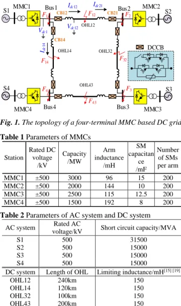
Fig. 1 shows the topology of a symmetrical monopole
four-terminal MMC based DC grid using OHL. Each converter adopts the half-bridge sub-module based MMC topology. For DC fault protection and isolation, the hybrid DCCBs proposed in [27] are implemented at the ends of each overhead line. The current limiting inductors are installed at the line side of DCCBs to limit the current rise rate during DC faults. The parameters of the MMCs, AC and DC systems are given in Table 1 and Table 2.
To facilitate selectivity, the tripping signals of DCCBs should be issued properly under different fault scenarios. Taking CB12 as an example, when DC faults happen at overhead line 12 (denote as internal line faults), CB12 should be tripped. When faults happen at other lines (denote as external line faults), CB12 should maintain the pre-fault state. In addition, when faults happen at DC bus1 (denote as DC bus faults), both CB12 and the adjacent CB14 should be tripped to isolate the faulted segments.
MMC1 MMC4 OHL12 MMC2 MMC3 CB12 CB14 S1 S4 S2 F1 F3 F12 F14 F32 F43 Vdc1 Vdc12 Idc12 Idc14 OHL14 OHL32 OHL43 F4 F2 Bus1 CB21Bus2 Bus4 Bus3 DCCB S3 Idc21
Fig. 1. The topology of a four-terminal MMC based DC grid.
Table 1 Parameters of MMCs Station Rated DC voltage /kV Capacity /MW Arm inductance /mH SM capacitan ce /mF Number of SMs per arm MMC1 ±500 3000 96 15 200 MMC2 ±500 2000 144 10 200 MMC3 ±500 2500 115 12.5 200 MMC4 ±500 1500 192 8 200 Table 2 Parameters of AC system and DC system
AC system Rated AC
voltage/kV Short circuit capacity/MVA
S1 500 31500
S2 500 15000
S3 500 15000
S4 500 15000
DC system Length of OHL Limiting inductance/mH[15] [19]
OHL12 240km 150
OHL14 120km 150
OHL32 100km 150
OHL43 200km 150
2.2. Frequency Difference during DC Line and DC Bus Faults
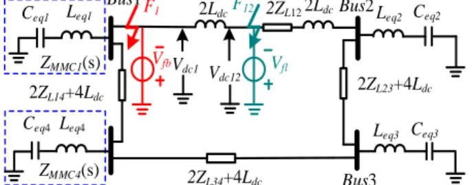
The equivalent circuit of the DC grid in frequency-domain can be drawn in Fig. 2 [15]-[19]. As shown, Leqi and Ceqi are
the equivalent inductance and capacitance of i th MMC station. ZL12 is the line reactance between station 1 and 2. Vdc1
and Vdc12 denote the transient voltages at the DC bus side and
line side, respectively. Vfb and Vfl represent the fault
3 respectively. ZL23, ZL34, ZL41 represent the equivalent reactance
(including the current limiting inductance, line inductance and resistance) of the OHL 23, 34 and 41, respectively.
Vdc1 2Ldc Vfb Leq4 Ceq1 Ceq4 Vdc12 2ZL122Ldc Leq3 Ceq3
Leq1 Leq2 Ceq2
Bus1 Bus2 2ZL34+4Ldc Bus3 ZMMC1(s) ZMMC4(s) F1 2ZL14+4Ldc 2ZL23+4Ldc F12 Vfl
Fig. 2. The equivalent circuit of DC grid when fault occurs.
As for the internal DC line faults (F12), the ratio of Vdc1 and Vdc12 in frequency-domain can be obtained in Fig. 3(a)
according to [15]. Based on Fig. 3(a), it can be seen that the high-frequency components in Vdc12 (DC line voltage) is
larger than those in Vdc1 (DC bus voltage) under DC line
faults.
As for the DC bus faults (F1), the ratio of Vdc1 and Vdc12 in
frequency-domain can be expressed as MMC2 ( ) 2 ( ) 4 2 ( ) || ( ) dc12 dc dc1 dc L12 3 V s sL V s sL Z Z s Z s (1)
where Z3(s)=ZMMC3(s)+2ZL23(s)+4sLdc. The equivalent
reactance ZMMC(s) of a MMC converter can be expressed as
[13][19] MMC 0 0 1 ( ) (2 ) 3 2 N Z s sL sC (2)
where L0 and C0 are the arm inductance and sub-module
capacitance respectively. By combining (1) and (2), the magnitude-frequency characteristic of the transfer function
Vdc12(s)/Vdc1 (s) can be obtained, as shown in Fig. 3(b).
0 101 102 103 104 105 106 107 -3 -2 -1 0 1 2 3 4 5 6 f / Hz lg | Vdc 12 ( s )/ Vdc 1 ( s )| a lg | Vdc 1 2 ( s )/ Vdc 1 ( s )| 0 -10 -8 -6 -4 -2 0 2 4 101 102 103 104 105 106 107 108 109 1010 f / Hz b
Fig. 3. The magnitude-frequency characteristics of
|Vdc12(s)/Vdc1 (s)|.
(a) DC line fault (b) DC bus fault
As shown in Fig. 3(b), the high-frequency components in
Vdc1 (DC bus voltage) are larger than those in Vdc12 (DC line
voltage) under DC bus fault.
To be concluded, due to the boundary effect provided by the current limiting inductances [15][16], the low-frequency and high-frequency components in DC line and bus voltages vary with DC fault locations. For internal line faults, the DC line voltage Vdc12 possesses large high-frequency components
while the DC bus voltage Vdc1 has small high-frequency
components. For DC bus faults, the characteristics are opposite with Vdc12 possessing small high-frequency
components and Vdc1 possessing large high-frequency
components. For external line faults, both DC line and bus voltages Vdc12 and Vdc1 have small high-frequency
components and large low-frequency components. Therefore, such DC fault characteristics offer a potential approach to identify the DC line and DC bus faults.
3. Design of Artificial Neural Network
Artificial neural networks have good adaptive and self-learning capabilities in pattern recognition problems. Usually, an ANN is composed of three layers, i.e. the input layer, the hidden layer and the output layer [23]-[26]. The number of neurons in the input layer is determined by the amount of input whereas the number of neurons in the output layer is determined by the output result. In this paper, to identify the fault location and fault type, five outputs are designed, corresponding to DC bus fault, transmission line fault, pole-to-pole DC fault, positive pole-to-ground DC fault and negative pole-to-ground DC fault, respectively. The first two outputs are designed for fault identification (DC bus or line faults), and the other three outputs are designed for faulty pole selection (PTP or PTG faults).
3.1. Design of Input Vector
As disclosed in section II, the characteristics of the DC line and bus voltages in frequency-domain vary with different fault locations. Thus, the discrete wavelet transform (DWT) is adopted to extract the high-frequency components in the transient DC voltages. Considering the frequency spectrum shown in Fig. 3(a) and the time delay of high decomposition level of WT, a 1-level DWT with 10 kHz sampling frequency is selected in this paper, which corresponds to 2.5-5kHz spectrum.
Applying DWT to the transient voltages, we can obtain the detailed coefficients for Vdc1 and Vdc12 under different DC
PTP faults, as shown in Fig. 4. The detailed coefficient of DWT represents the high-frequency components.
a b
Fig. 4. Detailed coefficients of transient voltages under
different PTP faults.
(a) DC line voltage Vdc12 (b) DC bus voltage Vdc1
Fig. 4 (a) shows that the detailed coefficients of DC line voltage Vdc12 in internal DC line fault (OHL 12) are much
larger than those in external line and DC bus faults. For Vdc1,
a larger detailed coefficient is observed in DC bus faults, as shown in Fig. 4 (b). Fig. 4 validates that the high-frequency components in DC line voltages are large during internal faults and small during external and bus faults, whereas the high-frequency components in DC bus voltage are large during bus faults. Denoting the detailed coefficient of transient voltage as d1(t), to further enlarge the difference of
high-frequency components, the square of detail coefficient
d1(t) are integrated within a time window as
Time(s) 1.5002 1.5006 1.501 1.5014 1.5018 -800 -400 0 400 800 d1 of V dc 1 2 / kV OHL12 OHL14 Bus1 1.5 1.5002 1.5004 1.5006 1.5008 -400 -300 -200 -100 0 100 200 300 Time(s) OHL12 OHL14 Bus1 d1 of Vdc 1 / k V 80 -60
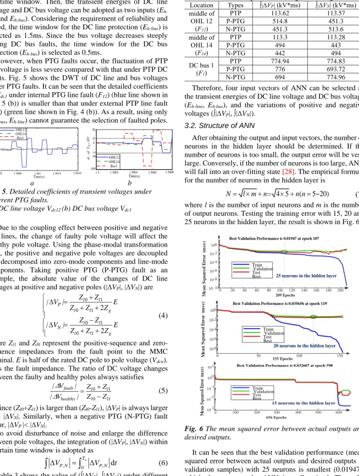
4 2 1 0 ( ) d w T h E
d n t (3)where Eh is denoted as the transient energy and Tw represents
the time window. Then, the transient energies of DC line voltage and DC bus voltage can be adopted as two inputs (E h-line and Eh-bus). Considering the requirement of reliability and
speed, the time window for the DC line protection (Eh-line) is
selected as 1.5ms. Since the bus voltage decreases steeply during DC bus faults, the time window for the DC bus protection (Eh-bus) is selected as 0.5ms.
However, when PTG faults occur, the fluctuation of PTP DC voltage is less severe compared with that under PTP DC faults. Fig. 5 shows the DWT of DC line and bus voltages under PTG faults. It can be seen that the detailed coefficients of Vdc1 under internal PTG line fault (F12) (blue line shown in
Fig. 5 (b)) is smaller than that under external PTP line fault (F14) (green line shown in Fig. 4 (b)). As a result, using only
(Eh-bus, Eh-line) cannot guarantee the selection of faulted poles.
a b
Fig. 5. Detailed coefficients of transient voltages under
different PTG faults.
(a) DC line voltage Vdc12 (b) DC bus voltage Vdc1
Due to the coupling effect between positive and negative DC lines, the change of faulty pole voltage will affect the healthy pole voltage. Using the phase-modal transformation [16], the positive and negative pole voltages are decoupled and decomposed into zero-mode components and line-mode components. Taking positive PTG (P-PTG) fault as an example, the absolute value of the changes of DC line voltages at positive and negative poles (|∆VP|, |∆VN|) are
0 1 0 1 0 1 0 1 2 2 l l P l l g l l N l l g Z Z | V | E Z Z Z Z Z | V | E Z Z Z (4)
where Zl1 and Zl0 represent the positive-sequence and
zero-sequence impedances from the fault point to the MMC terminal. E is half of the rated DC pole to pole voltage (Vdcn). Zg is the fault impedance. The ratio of DC voltage changes
between the faulty and healthy poles always satisfies
0 1 0 1 fault l l healthy l l | V | Z Z | V | Z Z (5)
Since (Zl0+Zl1) is larger than (Zl0-Zl1), |∆VP| is always larger
than |∆VN|. Similarly, when a negative PTG (N-PTG) fault
occur, |∆VP|< |∆VN|.
To avoid disturbance of noise and enlarge the difference between pole voltages, the integration of (|∆VP|, |∆VN|) within
a certain time window is adopted as
, 0 , d w T P N P N V V t
(6)Table 3 shows the value of (∫|∆VP|, ∫|∆VN|) under different
faults within a 1.5ms time window. It can be seen that the
∫|∆VP| and ∫|∆VN| are the same underPTP faults. Under PTG
faults, the value of the faulty pole is larger than that of the healthy pole.
Table 3 Variations of positive and negative voltages Location Types ∫|∆VP| (kV*ms) ∫|∆VN| (kV*ms) middle of OHL 12 (F12) PTP 113.62 113.57 P-PTG 514.8 451.3 N-PTG 451.3 513.6 middle of OHL 14 (F14) PTP 113.3 113.28 P-PTG 494 443 N-PTG 442 494 DC bus 1 (F1) PTP 774.94 774.83 P-PTG 776 693.72 N-PTG 694 774.96
Therefore, four input vectors of ANN can be selected as the transient energies of DC line voltage and DC bus voltage (Eh-line, Eh-bus), and the variations of positive and negative
voltages (∫|∆VP|, ∫|∆VN|). 3.2. Structure of ANN
After obtaining the output and input vectors, the number of neurons in the hidden layer should be determined. If the number of neurons is too small, the output error will be very large. Conversely, if the number of neurons is too large, ANN will fall into an over-fitting state [28]. The empirical formula for the number of neurons in the hidden layer is
= 4 5 ( 5~20)
N l m n n n (7) where l is the number of input neurons and m is the number of output neurons. Testing the training error with 15, 20 and 25 neurons in the hidden layer, the result is shown in Fig. 6.
Fig. 6 The mean squared error between actual outputs and
desired outputs.
It can be seen that the best validation performance (mean squared error between actual outputs and desired outputs in validation samples) with 25 neurons is smallest (0.01947), which demonstrates the ANN is well trained. Thus, the number of neurons in the hidden layer is selected as 25. The structure of the ANN is shown in Fig. 7.
1.5002 1.5006 1.501 1.5014 1.5018 -300 -200 -100 0 100 200 300 Time(s) d1 of V dc 1 2 ( kV ) OHL12 OHL14 Bus1 1.5 1.5002 1.5004 1.5006 1.5008 -100 -50 0 50 Time(s) d1 of V dc 1 / k V OHL12 OHL14 Bus1 20 -33 0 20 40 60 80 100 120 140 160 180 200 209 Epochs 10 -10 10-8 10-6 10-4 10-2 100
Best Validation Performance is 0.01947 at epoch 107
Train Validation Test Best M e a n S q u a re d E rr o r ( m s e )
25 neurons in the hidden layer
0 50 100 150 155 Epochs 10-8 10-6 10-4 10-2 100
Best Validation Performance is 0.035656 at epoch 119
Train Validation Test Best M e a n S q u a re d E rr o r ( m s e )
20 neurons in the hidden layer
0 100 200 300 400 500 600 656 Epochs 10-3 10-2 10-1 100
10 1 Best Validation Performance is 0.032607 at epoch 598
Train Validation Test Best M ea n S q u ar ed E rr or ( m se )
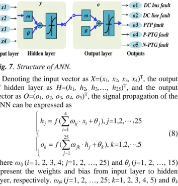
5 x1 x3 x4 ω θ
Input layer Hidden layer Output layer Outputs
y o o1 o2 o3 o4 o5 DC bus fault DC line fault P-PTG fault PTP fault N-PTG fault θ ω x2
Fig. 7.Structure of ANN.
Denoting the input vector as X=(x1, x2, x3, x4)T, the output
of hidden layer as H=(h1, h2, h3,…, h25)T, and the output
vector as O=(o1, o2, o3, o4, o5)T, the signal propagation of the
ANN can be expressed as
4 1 25 1 ( ), =1,2, 25 ( ), =1,2, ,5 j ij i j i k jk j k j h f x j o f h k
, (8) where ωij (i=1, 2, 3, 4; j=1, 2, …, 25) and 𝜃j (j=1, 2, …, 15)represent the weights and bias from input layer to hidden layer, respectively. ωjk (j=1, 2, …, 25; k=1, 2, 3, 4, 5) and 𝜃k
(k=1, 2, …, 5) represent the weight and bias from hidden layer
to output layer, respectively. f represents the activation function, where the tansig function shown below is adopted to reduce the training error.
2 2 ( ) = 1 1 n f x e (9)
3.3. Offline Training Process of ANN
The training process of the ANN includes two parts:
forward propagation of signals and back propagation of errors. Firstly, the inputs X=(x1, x2, x3, x4)T are transformed
into per-unit form as
min max min max min max min 2( ) 1, 1, i i i i i i i i i x x x x x x x x x (10) where ximax and ximin are the maximum and minimum value of
the sampled data of xi. Then, the inputs propagate to the
hidden and output layers.
The five outputs of the ANN correspond to DC bus fault, line fault, positive PTG fault, negative PTG fault and pole-to pole-fault, and their values are represented by 0 and 1. For example, if a PTP fault occurs at DC bus, the output vectors of o1 and o3 are set to 1 while the others are set to 0. By
comparing the desired outputs with calculated values, the weights and bias are adjusted by error back propagation. Through continuously adjusting the bias and weights, the ANN ensures the difference between the expected output and real output to satisfy the accuracy requirements, and thus establishes the mapping relationship between the faults and the output values.
With regard to the collection of training samples, different fault conditions including fault resistances, fault types, fault distances and noise are considered to train the ANN offline. Taking DCCB 12 as an example, PTP, P-PTG, N-PTG DC faults along OHL 12 and OHL 14 are applied at every 10% interval (0, 10%, 20%, …, 100% of the line) to obtain the training data. Then, samples are input to the ANN to train the network. The statistical results are given in Table 4.
Table 4 Samples for offline training of ANN Samples
Signal-to-noise ratio Locations Fault resistance/Ω (PTP fault, P-PTG and N-PTG faults) Training samples: 450 cases Validation samples: 150 cases No noise Every 10% of OHL 12 0.001, 30, 150, 210 Bus 1 0.001, 10, 30, 50,70,90,110,130, 150, 170, 190, 210 Every 10% of OHL 14 0.001, 30, 150, 210 30db Every 10% of OHL 12 0.001, 30, 150, 210 Bus 1 0.001, 10,30, 50,70,90,110,130,150,170, 190, 210 Every 10% of OHL 14 0.001, 30, 150, 210 Test samples: 216 cases No noise Every 20% of OHL 12 60,180 Bus 1 5, 15, 35, 55, 75, 95, 115, 135, 145, 175, 195, 215 Every 20% of OHL 14 60, 180 30db Every 20% of OHL 12 60, 180 Bus 1 5, 15, 35, 55, 75, 95, 115, 135, 145, 175, 195, 215 Every 20% of OHL 14 60, 180
Table 5 shows the outputs of the ANN under some internal DC line faults. As can be seen, although weights and bias are trained well, the outputs cannot be an ideal 0 or 1. Thus, a classifier is designed at the output stage as
1, 0.3 ( ) 1 0, j k f y o else (11)
When the offline training of the ANN is completed, it can then be used for fault detection online. Thus, the training time is not an important issue. Based on the aforementioned analysis, the overall protection flowchart is designed as shown in Fig. 8.
A fault start-up element is employed to determine the starting point of WT. In this paper, the rate of change of DC line voltage (dVdc/dt) is selected as the start-up element:
dc set
dV dtD (12)
When DC fault happens, the DC voltage will drop quickly. Once detecting dVdc/dt is smaller than the threshold, the first
sampling is conducted, thereby obtaining the input of ANN.
The practical protection system embedding the ANN based fault detection algorithm is shown in Fig. 9. The measured analog signals from the voltage transformers (VT) are delivered to the sampling circuit in real-time and then they are transformed into digital signals by the A/D transform. The digital signals are processed in the signal process unit. Once the fault start-up element is activated, a real-time WT will be employed to process the sampled signal with 1.5ms time window. Subsequent to the signal processing, the ANN input vectors will be obtained. On receiving the input vectors of ANN, the trained-well ANN algorithm written in FPGA (field programmable gate array) will output the results. Then, the results will determine the operation of DCCBs.
6 Table 5 Outputs of ANN
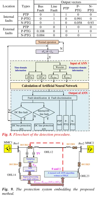
Location Types Output vectors Bus Fault Line Fault PTP P-PTG N- PTG Internal faults PTP 0 1 1 0 0 P-PTG 0 1 0 0.991 0 N-PTG 0 1 0 0.058 0.93 External faults PTP 0 0 1 0 0 P-PTG 0.108 0 0 1 0 N-PTG 0.004 0 0 0 1 Y
Fault identification & Fault discrimination
| VP|
Wavelet
Calculation of Artificial Neural Network
| VN| Eh-line Eh-bus DC Bus fault N Input of ANN Output of ANN Internal DC line fault DC line protection acts PTP fault P-PTG N-PTG Normal operation N DC bus protection acts Y Y Time-domain information Frequency-domain information N
Fig. 8. Flowchart of the detection procedure.
MMC1 OHL12 DCCB14 OHL14 DCCB12 Bus1 DCCB21 Bus2 MMC2 DCCB23 OHL23 TV Sampling circuit Signal processing unit (DSP+FPGA) Vdc Eh-line, Eh-bus,| VP|,| VN|
A trained well ANN algorithm written in FPGA 0 and 1 A/D
transverter
Fig. 9. The protection system embedding the proposed
method.
4. Simulation Validation
A four-terminal MMC based DC grid shown in Fig. 1 is built in PSCAD/EMTDC. MMC1 controls the DC voltage, and the other stations adopt active and reactive power control. Defining positive active power as flowing from converters into the DC grid and positive reactive power as converters providing capacitive reactive power to the AC networks, the active power of MMC2MMC4 are 0.95pu, 0.95pu and -0.95pu, respectively, whereas the reactive power of MMC1-MMC4 are 0.1pu, 0.15pu, 0.1pu and 0.1pu, respectively. The mother wavelet is selected as sym8 with presenting the closest match to the pattern of the fault signal [29]. The DC current limiting inductance should be selected to protect the MMC from overcurrent during the DC fault detection period in the events of DC line faults. In this paper, it is selected as 150mH.
Each MMC implements the overcurrent protection. Once the arm currents of MMC exceed the threshold (two times of the rated value), the MMC will be blocked.
4.1. Identification of DC Line Fault and DC Bus Fault
Applying different DC faults with 0.01Ω resistance at DC bus1 and at different locations along OHL 12 and OHL 14, the identification results for CB12 are shown in Table 6.
During the internal faults (faults on OHL 12), the PTP and PTG fault are accurately identified and CB12 can be tripped. As shown in Table 6, the detection time delay increases slightly with the increase of fault distance.
Fig. 10 shows the simulation results under a PTP fault occurring at the one-fourth of OHL12 at 1.5s. Fig. 10 (a) shows that CB12 receives the tripping command at 1.5018s (0 stands for closing while 1 stands for tripping). Fig. 10(b) shows that the peak value of the fault line current is almost 6kA. Fig. 10(c) shows the DC power of MMC1 and it can be seen that due to the fast isolation of DC fault lines, MMC1 restores rated power transmission within 200-300 ms. Fig. 10(d) shows that the arm currents are within the safe range during the detection period.
During the external faults (faults on OHL 14), the fault types are successfully identified, and neither the DC line protection nor DC bus detection activates. Thus, CB12 remains on-state, as shown in Table 6.
a Idc 12 / k A 1.498 1.5 1.502 1.504 1.506 1.508 1.51 1.512 -2 0 2 4 6 Time(s) b c Iarm / kA Iarm_up (C) Iarm_up (B)
Iarm_dn (A) Iarm_dn (C) Iarm_dn (B) Iarm_up (A) Times (s) 1.495 1.496 1.497 1.498 1.499 1.5 1.501 1.502 1.503 -4 -2 0 2 4 -3.01 d
Fig. 10. The waveforms under PTP fault on OHL 12.
(a) Firing signal of CB12 (b) DC current on OHL 12 (c) DC
power of MMC1(d)Arm currents of MMC1.
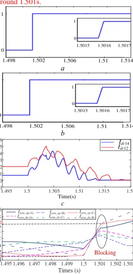
Fig. 11 shows the simulation results under a PTP DC bus
1.498 1.502 1.506 1.51 1.514 0 1 1.5018 1.5019 1.502 0 1 St at e of CB 12 Time(s) 1.4 1.6 1.8 2 2.2 2.4 -1.2 -1 -0.8 -0.6 -0.4 -0.2 P / pu Time(s)
7 fault occurring at 1.5s. Since the DC bus fault is identified by
the ANN, CB12 and CB14 are tripped. Fig. 11 (a)-(b) shows that CB12 and CB14 received the tripping command at 1.50156s. Fig. 11 (c) show that due to the quick-action of the DCCBs, the peak value of the fault line current is limited to 5kA (2.5pu of rated value). Fig. 11(d) shows that the arm currents of MMC1 exceed the threshold and MMC1 is blocked around 1.501s. a b Time(s) Idc / k A 1.495 1.5 1.505 1.51 1.515 1.52 -1 0 1 2 3 4 5 6 I dc14 Idc12 c Iarm / kA -4 Iarm_up (C) Iarm_up (B)
Iarm_dn (A)Iarm_up (A) Iarm_dn (C) Iarm_dn (B)
Blocking Times (s) 1.495 1.496 1.497 1.498 1.499 1.5 1.501 1.502 1.503 -2 0 2 4 6 8 10 -3.01 6.02 d
Fig. 11. The waveforms under PTP fault at DC bus 1.
(a) Firing signal of CB12 (b) Firing signal of CB14 (c) DC currents Idc12 and Idc14 (d)Arm currents of MMC1.
4.2. Impact of AC faults on Fault detection
As for AC faults which are out of DC protection zone, the DC line and DC bus protection should not be activated. The proposed protection algorithm is tested by scanning different AC faults in different areas.
At 1.5s, single-phase (1PF), two-phase (2PF) and three-phase short circuit faults (3PF) are applied respectively. The results shown in Table 7 indicate that when AC faults occur, neither the DC line protection nor the DC bus protection will trigger. As fault resistance increases, the effect of AC faults on protection will be further diminished.
4.3. Impact of Change of Operating Conditions
Further tests are conducted to validate the robustness of the proposed ANN method under different operating conditions. At 1.5s, the power command of each converter reverses and a permanent PTP DC fault is applied at the middle of OHL 12 at 4s. The simulation results are shown in Fig. 12.
Fig. 12 (a) shows the active power of each converter starts to reverse at 1.5s. After minor fluctuations, the active power of each converter reaches steady state around 2s. At 4s, since a DC fault occurs, there are large transients in active power. Fig. 12 (b) shows the tripping order of CB 12. As can be seen, during the fluctuation of active power, the protection will not be falsely activated. At 4s, since a PTP fault occurs, there are large transients in DC line voltage and active power, resulting in the activation of DC line protection of CB 12. Therefore, the method can be adopted to different modes of operation.
5. Performance Evaluation
5.1. Performance under High-Resistance Faults
To test the effectiveness of the ANN under non-metallic faults, different fault resistances are applied and the calculation results are shown in Table 8. As can be seen, the proposed ANN based method can correctly identify the fault resistance as high as 350Ω and determine the fault types.
As for higher fault resistance, such as 400Ω and 500Ω, the success rate of ANN for fault detection will decrease, as shown in Fig. 13. However, the fault current under such resistance is relatively small, which has a lower requirement for protection speed and the fault detection can be achieved by the backup protection.
Table 6 Outputs of ANN and protection states under different DC faults Location types Fault
Outputs of ANN DC bus protection (Bus1) DC line protection (CB12) Detection delay (ms) Bus
Fault Line Fault PTP P-PTG PTG N-1/4 of OHL12 PTP 0 1 1 0 0 No-action Trip 1.8 P-PTG 0 1 0 1 0 No-action Trip 1.8 2/3 of
OHL12 P-PTG PTP 0 0 1 1 0 1 0 1 0 0 No-action No-action Trip Trip 2 2 3/4 of
OHL12
PTP 0 1 1 0 0 No-action Trip 2.18
P-PTG 0 1 0 1 0 No-action Trip 2.18
1/4 of
OHL14 P-PTG PTP 0 0 0 0 0 1 0 1 0 0 No-action No-action No-action No-action 1.66 1.66 2/3 of OHL14 PTP 0 0 1 0 0 No-action No-action 1.82 P-PTG 0 0 0 1 0 No-action No-action 1.82 3/4 of OHL14 PTP 0 0 1 0 0 No-action No-action 1.92 P-PTG 0 0 0 1 0 No-action No-action 1.92
DC bus 1 P-PTG PTP 1 1 0 0 0 1 0 1 0 0 Trip Trip No-action No-action 1.56 1.56
1.498 1.502 1.506 1.51 1.514 0 1 1.5015 1.5016 1.5017 0 1 Time(s) S ta te o f CB 12 1.498 1.502 1.506 1.51 1.514 0 1 1.5015 1.5016 1.5017 0 1 Time(s) St at e of CB 14
8 Table 7 Protection states under different AC faults
Location Fault types Fault resistance DC bus protection (Bus1) DC line protection (CB12) S1 1PF 0.01Ω No-action No-action 2PF 0.01Ω No-action No-action 3PF 0.01Ω No-action No-action S2 1PF 0.01Ω No-action No-action 2PF 0.01Ω No-action No-action 3PF 0.01Ω No-action No-action S4 1PF 0.01Ω No-action No-action 2PF 0.01Ω No-action No-action 3PF 0.01Ω No-action No-action S1 1PF 50Ω/200 Ω No-action No-action 2PF 50Ω/200 Ω No-action No-action 3PF 50Ω/200 Ω No-action No-action
5.2. Performance under Noise Disturbance
Since Eh-line and Eh-bus are obtained based on
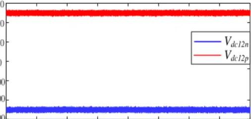
high-frequency information, their accuracy could be affected by high-frequency noise in measurements. To test the effectiveness of the proposed method under measurement noise, an 18db white noise is added to the measured DC bus and DC pole voltages, as shown in Fig. 14.
Applying different DC faults with different fault resistances and noise, the identification results of ANN are shown in Table 9. As can be seen, the noise does not lead to false operation of ANN, which is one of the main advantages of the proposed ANN based method. It is owing to the following two factors. Firstly, the offline training samples have considered the impact of noise, in which the training weights and bias were adjusted to the noise. Secondly, although the DWT method is affected by the high-frequency disturbance, the introduced time domain inputs of (∫|∆VP|, ∫|∆VN|) improves the immunity of ANN to noise.
5.3. Sensitivity against the size of DC inductance
To evaluate the sensitivity of the proposed method versus the size of DC inductance, different DC current limiting inductances varying from 0.1H to 0.45H for Ldc12 are tested.
The identification results of the ANN are shown in Table 10. As can be seen, the internal, external and DC bus fault are properly identified.
It can be concluded that with large current limiting inductors, the high-frequency differences of detected voltages between internal and external faults will become more obvious, which improves the accuracy of the proposed method.
5.4. Time Delay of Fault Detection
For MMC based DC grids, fast fault identification is required. In this paper, the ANN is trained using various offline data. Once offline training is completed, the speed of online detection mainly depends on the time window and the fault distance and resistance. For nearby PTP and PTG faults, the detection delays are largely the same. However, when PTG faults with high fault resistance occur at the end of the lines, the propagation delay is slightly longer. Thus, the detection delay is longer.
When the fault occurs at the end of OHL 12 with 350Ω fault resistance, the longest detection time delay observed is only 2.48ms, as disclosed in Table 8. Therefore, the method proposed in this paper can provide fast fault detection.
a b
Fig. 12. Waveforms under change of operating conditions. (a) Active power of each converter (b) Firing signals of CB12
0 10 20 30 40 50 s u c c e s s r ate (%) 60 70 80 90 100 82.3% 100% 100% 150Ω 100%
internal faults (264cases) external faults All Samples
200Ω 250Ω 300Ω 77.9% 67.7% 350Ω 400Ω 450Ω 500Ω 94% 89% 92.42% 87.5% 84.5% (136cases) 78% (400cases) Fault resistance 100% 100%
Fig. 13. The success rate of ANN under different fault resistances
1 1.5 2 2.5 3 3.5 4 -4 -3 -2 -1 0 1 2 3 MMC1 4.5 MMC2 MMC3 MMC4 Time(s) P /pu 3.998 4.002 4.006 4.01 4.014 0 1 4.0019 4.002 4.0021 0 1 St at e of CB 12 Time(s)
9 Time(s) 1.5 1.6 1.7 1.8 1.9 2 600 800 1000 1200 1400 Vd c 1 / k V a b
Fig. 14. Waveforms of DC voltages with 18db noise. (a) DC bus voltage (b) Pole voltages of DC lines
Table 8 Outputs of ANN and protection states under different DC faults with different fault resistances
Location resistance Fault Fault types
Output of ANN DC line
protection (CB12) DC bus protection (Bus1) Detection delay (ms) Bus Fault Line Fault PTP P-PTG N-PTG
1/4 of OHL 12 50Ω PTP 0 1 1 0 0 Trip No-action 1.8 P-PTG 0 1 0 1 0 Trip No-action 1.8 N-PTG 0 1 0 0 1 Trip No-action 1.8 200Ω PTP 0 1 1 0 0 Trip No-action 1.8 P-PTG 0 1 0 1 0 Trip No-action 1.8 N-PTG 0 1 0 0 1 Trip No-action 1.8 350Ω PTP 0 1 1 0 0 Trip No-action 1.8 P-PTG 0 1 0 1 0 Trip No-action 1.8 N-PTG 0 1 0 0 1 Trip No-action 1.8 1/2 of OHL 12 50Ω PTP 0 1 1 0 0 Trip No-action 2 P-PTG 0 1 0 1 0 Trip No-action 2 N-PTG 0 1 0 0 1 Trip No-action 2 200Ω PTP 0 1 1 0 0 Trip No-action 2 P-PTG 0 1 0 1 0 Trip No-action 2 N-PTG 0 1 0 0 1 Trip No-action 2 350Ω PTP 0 1 1 0 0 Trip No-action 2 P-PTG 0 1 0 1 0 Trip No-action 2 N-PTG 0 1 0 0 1 Trip No-action 2 3/4 of OHL 12 50Ω PTP 0 1 1 0 0 Trip No-action 2.18 P-PTG 0 1 0 1 0 Trip No-action 2.18 N-PTG 0 1 0 0 1 Trip No-action 2.18 200Ω PTP 0 1 1 0 0 Trip No-action 2.18 P-PTG 0 1 0 1 0 Trip No-action 2.28 N-PTG 0 1 0 0 1 Trip No-action 2.28 350Ω PTP 0 1 1 0 0 Trip No-action 2.18 P-PTG 0 1 0 1 0 Trip No-action 2.28 N-PTG 0 1 0 0 1 Trip No-action 2.28 100% of OHL 12 50Ω PTP 0 1 1 0 0 Trip No-action 2.38 P-PTG 0 1 0 1 0 Trip No-action 2.38 N-PTG 0 1 0 0 1 Trip No-action 2.38 200Ω PTP 0 1 1 0 0 Trip No-action 2.38 P-PTG 0 1 0 1 0 Trip No-action 2.48 N-PTG 0 1 0 0 1 Trip No-action 2.48 350Ω PTP 0 1 1 0 0 Trip No-action 2.38 P-PTG 0 1 0 1 0 Trip No-action 2.48 N-PTG 0 1 0 0 1 Trip No-action 2.48 DC bus 1 50Ω PTP 1 0 1 0 0 No-action Trip 1.56 P-PTG 1 0 0 1 0 No-action Trip 1.56 N-PTG 1 0 0 0 1 No-action Trip 1.56 200Ω PTP 1 0 1 0 0 No-action Trip 1.56 P-PTG 1 0 0 1 0 No-action Trip 1.56 N-PTG 1 0 0 0 1 No-action Trip 1.56 350Ω PTP 1 0 1 0 0 No-action Trip 1.56 P-PTG 1 0 0 1 0 No-action Trip 1.56 N-PTG 1 0 0 0 1 No-action Trip 1.56
5.5. Comparisons with existing methods
1) Comparison with the transient voltage and wavelet transform based method proposed in [15].
Taking CB12 as an example, apply a metallic PTP fault at F12 at 2s. The measured transient energy of the DC line
voltage is shown Fig. 15 (a). Apply a metallic PTP fault at
bus 2 (F2) with 20db white noise at 2s. The measured transient
energy is shown in Fig. 15 (b). It can be seen that the Eh
during a DC bus fault (F2) is higher than that during an
internal fault (F12), which indicates the false operation of the
protection system.
2) Comparison with the ratio of the transient voltages (ROTV) method proposed in [16].
1 1.05 1.1 1.15 1.2 1.25 1.3 1.35 1.4 -600 -400 -200 0 200 400 600 Vdc12p Vdc12n Vdc 12 p (n ) / kV Times(s)
10 Apply a PTG fault with 200Ω resistance at the positive pole
of OHL12 (F12) at 2s. Using equation (2) in reference [16],
the calculated ROTV is 22. However, when applying a
metallic PTP fault at F2, the calculated ROTV is 21.5. These
values are so close that it is difficult to set the threshold for DCCB 12 using ROTV method.
Table 9 Outputs of ANN and protection states with noise Noise
(db)
Fault resistanc
e Location Fault types
Outputs of ANN DC bus protection (Bus1) DC line protection (CB12) Bus Fault Line Fault PTP P-PTG N-PTG 30 0.01 Ω 1/4 of OHL12 PTP 0 1 1 0 0 No-action Trip P-PTG 0 1 0 1 0 No-action Trip 1/4 of OHL14 PTP 0 0 1 0 0 No-action No-action P-PTG 0 0 0 1 0 No-action No-action
DC bus 1 P-PTG PTP 1 1 0 0 1 0 0 1 0 0 Trip Trip No-action No-action
200 Ω 1/4 of OHL12 PTP 0 1 1 0 0 No-action Trip P-PTG 0 1 0 1 0 No-action Trip 1/4 of OHL14 PTP 0 0 1 0 0 No-action No-action P-PTG 0 0 0 1 0 No-action No-action DC bus 1 P-PTG PTP 1 1 0 0 1 0 0 1 0 0 Trip Trip No-action No-action
20 0.01 Ω 1/4 of OHL12 PTP 0 1 1 0 0 No-action Trip P-PTG 0 1 0 1 0 No-action Trip 1/4 of OHL14 PTP 0 0 1 0 0 No-action No-action P-PTG 0 0 0 1 0 No-action No-action
DC bus 1 PTP 1 0 1 0 0 Trip No-action
P-PTG 1 0 0 1 0 Trip No-action
200 Ω
1/4of
OHL12 P-PTG PTP 0 0 1 1 1 0 0 1 0 0 No-action No-action Trip Trip 1/4 of
OHL14
PTP 0 0 1 0 0 No-action No-action
P-PTG 0 0 0 1 0 No-action No-action DC bus 1 P-PTG PTP 1 1 0 0 1 0 0 1 0 0 Trip Trip No-action No-action
18 0.01 Ω 1/4 of OHL12 PTP 0 1 1 0 0 No-action Trip P-PTG 0 1 0 1 0 No-action Trip 1/4 of OHL14 PTP 0 0 1 0 0 No-action No-action P-PTG 0 0 0 1 0 No-action No-action
DC bus 1 P-PTG PTP 1 1 0 0 1 0 0 1 0 0 Trip Trip No-action No-action
200 Ω 1/4of OHL12 PTP 0 1 1 0 0 No-action Trip P-PTG 0 1 0 1 0 No-action Trip 1/4 of OHL14 PTP 0 0 1 0 0 No-action No-action P-PTG 0 0 0 1 0 No-action No-action DC bus 1 P-PTG PTP 1 1 0 0 1 0 0 1 0 0 Trip Trip No-action No-action
Table 10 Outputs of ANN and protection states considering change of current limiting inductances
Arm inductance/
H
Location resistance Fault types Fault
Outputs of ANN DC bus
protection (Bus1) DC line protection (CB12) Bus Fault Line Fault PTP P-PTG N-PTG 0.1 1/2 of OHL12 100Ω PTP 0 1 1 0 0 No-action Trip P-PTG 0 1 0 1 0 No-action Trip 1/2 of OHL14 100Ω PTP 0 0 1 0 0 No-action No-action P-PTG 0 0 0 1 0 No-action No-action
DC bus 1 100Ω P-PTG PTP 1 1 0 0 1 0 0 1 0 0 Trip Trip No-action No-action
0.45 1/2 of OHL12 100Ω PTP 0 1 1 0 0 No-action Trip P-PTG 0 1 0 1 0 No-action Trip 1/2 of OHL14 100Ω PTP 0 0 1 0 0 No-action No-action P-PTG 0 0 0 1 0 No-action No-action
DC bus 1 100Ω P-PTG PTP 1 1 0 0 1 0 0 1 0 0 Trip Trip No-action No-action
3) Comparison with the rate of change of voltage (ROCOV) method proposed in [17].
Apply the same PTG fault at F12, the measured ROCOV
11 Fig. 16 (a). It can be seen that the highest ROCOV observed
is 1350 kV/ms. Apply a metallic PTP fault at bus 2 (F2) at
2s. The measured ROCOV at the line side of the current limiting inductor is shown in Fig. 16 (b). It can be seen that the highest ROCOV is higher than 1450 kV/ms. Thus, the ROCOV during a bus fault (F2) is higher than that during an
internal fault (F12). Using only the ROCOV criterion, the
internal faults with high fault resistance cannot be identified.
Based on the analysis above, it can be concluded that the using the method proposed in this paper, the protection scheme has the capability of fault resistance endurance and anti-disturbance.
a
b
Fig. 15. Simulation results using transient energy method.
(a) Eh during internal DC line fault (F12) (b) Eh during DC bus fault (F2)
a
b
Fig. 16. Simulation results using ROCOV method.
(a) ROCOV during internal DC line fault (F12) (b) ROCOV during DC bus fault (F2)
6. Conclusions
A DC fault protection scheme using ANN approach for MMC based DC grid is proposed in this paper. To decrease
the number of neural networks and avoid complicated training process, the input signals are preprocessed by DWT. It extracts information from the transient DC voltages in both time and frequency domains, leading to simplified neural network design, reduction of the volume of ANN data and robust to noise disturbance and fault resistance. The maximum tolerated fault resistance is as high as 350Ω and the noise disturbance is as high as 18db. The output signals are generated by the fault classifier to command the DCCBs. The proposal ANN method can not only identify DC line and DC bus faults, but also select faulted poles. The ANN is trained using a large number of offline cases, so the online detection time is fast (in less than 2.5ms). The ANN based protection scheme avoids the difficulties in thresholds setting that lacks theoretical foundation. Quantities of simulation results demonstrate its accuracy not being affected by power reversal and AC faults.
7. Acknowledgments
This work is sponsored by the Joint Funds of National Natural Science Foundation of China (U1766211 and 51807071) and China Postdoctoral Science Foundation (2017M620320).
8. References
[1] Freytes, J., Akkari, S., Rault, P., et al.: ‘Dynamic Analysis of MMC-Based MTDC Grids: Use of MMC Energy to Improve Voltage Behavior,’ IEEE Trans. Power Del., 2019, 34, (1), pp. 137-148. [2] Xiang, W., Lin, W., Xu, L., et al.: ‘Enhanced Independent Pole
Control of Hybrid MMC-HVDC System,’ IEEE Trans. Power Del., 2018, 33, (2), pp. 861-872.
[3] Wang, Y., Wang, C., Xu, L., et al.: ‘Adjustable Inertial Response
from the Converter with Adaptive Droop Control in DC Grids,’ IEEE Trans Smart Grid, 2019, 10, (3), pp. 3198-3209.
[4] Tang, G., He, Z., Pang, H., et al.: ‘Basic topology and key devices of the five-terminal DC grid,’ CSEE Journal of Power and Energy Syst., 2015, 1, (2), pp. 22-35.
[5] Han, X., Sima, W., Yang, M., et al.: ‘Transient Characteristics Under Ground and Short-Circuit Faults in a ±500kV MMC-Based HVDC System with Hybrid DC Circuit Breakers,’ IEEE Trans. Power Del.,
2018, 33, (3), pp. 1378-1387.
[6] Mohanty, R., Pradhan, A. K.: ‘A Superimposed Current Based Unit Protection Scheme for DC Microgrid,’ IEEE Trans Smart Grid, 2018, 9, (4), pp. 3917-3919.
[7] Jahn, I., Johannesson, N., Norrga, S.: ‘Survey of methods for selective DC fault detection in MTDC grids,’ presented in 13th IET International Conf. on AC and DC Power Transm., Manchester, UK, 2017, pp. 1-7.
[8] Huang, Q., Zou, G., Wei, X., et al.: ‘A Non-unit Line Protection Scheme for MMC-based Multi-terminal HVDC grid,’ Int. J. Elect. Power Energy Syst., 2019, 107, pp. 1-9.
[9] Tang, L., Dong, X., Shi, S., et al.: ‘A high-speed protection scheme for the DC transmission line of a MMC-HVDC grid,’ Elect. Power Syst. Research, 2019, 168, pp. 81-91.
[10] Tong, N., Lin, X., Li, Y., et al.: ‘Local Measurement-Based Ultra-High-Speed Main Protection for Long Distance VSC-MTDC,’ IEEE Trans. Power Del., 2019, 34, (1), pp. 353-364.
[11] Jamali, S., Mirhosseini, S. S.: ‘Protection of transmission lines in multi-terminal HVDC grids using travelling waves morphological gradient,’ Int. J. Elect. Power Energy Syst., 2019, 108, pp. 125-134 [12] Yeap, Y. M., Ukil, A.: ‘Fault detection in HVDC system using short
time fourier transform,’ IEEE Power and Energy Society General Meeting, Boston, USA, 2016, pp. 1-5.
[13] Kong, M., Pei, X., Pang, H., et al.: ‘A lifting wavelet-based protection strategy against DC line faults for Zhangbei HVDC Grid in China,’ 19th European Conf. on Power Electron. and Applica. (EPE'17 ECCE Europe), Warsaw, Poland, Sep. 2017, pp. 1-11. [14] Zhao, P., Chen, Q., Sun, K., ‘A novel protection method for
VSC-MTDC cable based on the transient DC current using the S
2 2.0005 2.001 2.0015 2.002 0 1000 2000 3000 Eh Time(s) 1.9 1.95 2 2.05 0 1000 2000 3000 4000 Eh Time(s) 1.995 2 2.005 2.01 -1500 0 1500 Time(s) dV 12 /dt ( kV /ms ) 1.9999 2 2.0001 -1350 0 1.995 2 2.005 2.01 -1500 0 1500 Time(s) dV 12 /dt ( kV /ms ) 2 2.001 2.002 -1450 0
12 transform,’ Int. J. Elect. Power Energy Syst., 2018, 97, pp. 299-308
[15] Xiang, W., Yang, S., Xu, L., et al.: ‘A Transient Voltage based DC
Fault Line Protection Scheme for MMC based DC Grid Embedding DC Breakers,’ IEEE Trans. Power Del., 2019, 34, (1), pp. 334-345 [16] Liu, J., Tai, N., Fan, C.: ‘Transient-Voltage Based Protection Scheme
for DC Line Faults in Multi-terminal VSC-HVDC System,’ IEEE Trans. Power Del., 2017, 32, (3), pp. 1483-1494.
[17] Sneath, J., Rajapakse, A.: ‘Fault detection and Interruption in an earthed HVDC grid using ROCOV and hybrid DC breakers,’ IEEE Trans. Power Del., 2016, 31, (3), pp. 973-981.
[18] Li, R., Xu, L., Yao, L.: ‘DC fault detection and location in meshed multi-terminal HVDC systems based on DC reactor voltage change rate,’ IEEE Trans. Power Del., 2017, 32, (3), pp. 1516-1626. [19] Li, C., Gole, A. M., Zhao, C.: ‘A Fast DC Fault Detection Method
Using DC Reactor Voltages in HVdc Grids,’ IEEE Trans. Power Del., 2018, 33, (5), pp. 2254-2264.
[20] Tzelepis, D., Dysko, A., Fusiek, G., et al.: ‘Advanced fault location in MTDC networks utilising optically-multiplexed current measurements and machine learning approach,’ Int. J. Elect. Power Energy Syst., 2018, 97, pp. 319-333.
[21] Rui, B. J., Lacerda, V. A., Monaro, R. M., et al.: ‘Selective non-unit Protection Technique for Multiterminal VSC-HVDC Grids,’ IEEE Trans. Power Del., 2017, 27, (3), pp. 1583-1591.
[22] Santos, R. C., Blond, S. L., Coury, D. V., et al.: ‘A novel and comprehensive single terminal ANN based decision support for relaying of VSC based HVDC links,’ Electr. Power Syst. Research, 2016, 141, pp. 333-343.
[23] Yang, Q., Blond, S. L., Aggarwal, R., et al.: ‘New ANN method for multi-terminal HVDC protection relaying,’ Electr. Power Syst. Research, 2017, 148, pp. 192-201.
[24] Hossam-Eldin, A., Lotfy, A., Elgamal, M., et al.: ‘Artificial intelligence-based short-circuit fault identifier for MT-HVDC systems,’ IET Gener. Transm. Distrib., 2018, 12, (10), pp. 2436-2443 [25] Merlin, V. L. R., Santos, C. d., Blond, S. Le, et al.: ‘Efficient and robust ANN-based method for an improved protection of VSC-HVDC systems,’ IET Renewable Power Gener., 2018, 12, (13), pp. 1555-1562.
[26] Wang, J., Zheng X. Tai, N.: ‘DC Fault Detection and Classification Approach of MMC-HVDC Based on Convolutional Neural Network,’ 2018 2nd IEEE Conf. on Energy Internet and Energy Syst. Integration (EI2), Beijing, 2018, pp. 1-6.
[27] Derakhshanfar, R., Jonsson, T. U., Steiger, U., et al.: ‘Hybrid HVDC
breaker–A solution for future HVDC system,’ presented in CIGRE Session, Paris, 2014, pp.1-12.
[28] T.S. Dillon, D. Niebur, Neural Networks Applications in Power Systems, CRLPublishing, London, 1996.
[29] Yeap, Y. M., Geddada, N., Ukil, A.: ‘Analysis and Validation of Wavelet Transform Based DC Fault Detection in HVDC System,’