Monte Carlo Simulation of Solid-Fluid Phase Equilibria in Binary and Ternary Mixtures

(1)

ATTWOOD, BRIAN CHRISTOPHER. Monte Carlo Simulations of Solid-Fluid Phase

Equilib-ria in Binary and Ternary Mixtures. (Under the direction of Carol K. Hall)

The objective of this research is to study the solid-fluid phase equilibria of binary and

ternary mixtures using molecular simulation. Solid-fluid phase equilibria plays an important

role in many chemical processes, especially crystallization. This research provides insight into

the underlying phenomena that govern these processes.

We first calculate complete phase diagrams, that is showing the solid, liquid, and vapor

phases, for 29 binary mixtures of Lennard-Jones molecules characterized by different sets of

interaction parameters using the Gibbs Duhem integration technique. The impact of including

the possibility of a solid phase on the global phase behavior of such mixtures is investigated by

comparing the complete phase behavior calculated by simulation to the global phase diagram

calculated from a fluid-phase-only equation of state. Complete phase diagrams from each region

of the global phase diagram are presented and compared with the fluid-phase-only phase

be-havior for the same mixture. It is found that for mixtures in which the components have greatly

dissimilar critical temperatures, the presence of the solid phase significantly alters the fluid phase

equilibria. In those cases, the phase behavior classification based on experimental observations

should differ from that predicted by an equation of state approach.

The Gibbs Duhem integration technique is then extended to calculate ternary phase

dia-grams at constant temperature and pressure. We calculate solid-fluid phase equilibria for ternary

mixtures of Lennard-Jones molecules. The simulation parameters were selected to roughly

(2)

melting point and a slightly smaller diameter. The cross-species well-depth and diameter

be-tween the two diastereomers are varied to determine their impact on the phase equilibria. We

find that increasing the interspecies diameter up to the diameter of the larger diastereomer results

in a slight increase of the solubility of the solid phase. We also find that when the interspecies

well-depth is lowered to less than that of either of the diastereomers, the solid phase separates into

two solid solutions and consequently there is a region of three-phase coexistence in the ternary

phase diagram. Finally we calculate ternary phase diagrams at a series of temperatures for one

set of molecular parameters. As the temperature increases, we find that the three-phase region

decreases in size until it eventually disappears. For an equimolar mixture of diastereomers, there

is a range of temperature and solvent concentration at which only one of the diastereomers will

precipitate, thus effecting a separation of the diastereomers. As the temperature is decreased the

(3)

and Ternary Mixtures

by

BRIAN CHRISTOPHER ATTWOOD

A dissertation submitted to the Graduate Faculty of North Carolina State University

in partial fulfillment of the requirements for the Degree of

Doctor of Philosophy

Chemical Engineering

Raleigh, NC 27695

2003

APPROVED BY:

Carol K. Hall Keith E. Gubbins Chair of Advisory Committee

(4)

Biography

The author was born in Troy, New York on April 27, 1975. He is the eldest son of Richard

and Dorothea Attwood and has two brothers, Jason and Kristopher. He received a B.S. degree in

chemical engineering from the State University of New York at Buffalo in May, 1997. In August,

1997, he was admitted to North Carolina State University to pursue graduate studies in Chemical

Engineering. On June 21, 1998, he married Karen Elizabeth Zawoysky of Clifton Park, New

York. He received an M.S. degree in chemical engineering from North Carolina State University

(5)

Acknowledgments

Through their support and encouragement, many people have contributed to the preparation

of this thesis. It gives me great pleasure to acknowledge them here.

First, I would like to thank my advisor, Professor Carol Hall. This thesis could not have

been completed without the insights I gained from discussions we had on both technical and

personal matters. Professor Hall is obviously very concerned about the welfare and success of

her students and I am grateful to be one of her students. I would also like to thank her for

obtaining the funding necessary to support me and my research for the past several years.

I thank the Office of Energy Research, Basic Sciences, Chemical Science Division of the

U.S. Department of Energy and the donors of the Petroleum Research Fund administered by the

American Chemical Society for their financial support for the research included in this thesis.

I am grateful to Julie McCormick, Andrew Schultz, Alex Marchut, Aysa Akad, and Arthi

Jayaraman for their parts in our joint effort to keep our computers running smoothly. I would also

like to thank the other members of our research group, past and present, for their friendship and

encouragement. To my other colleagues in the department with whom I have interacted, I thank

you for the support you have shown my work and the enjoyment you have given me socializing

outside of the office.

To my family and friends, I am especially grateful for the love and encouragement that you

have given me while in graduate school. Although I do not get to see you as much as I would

like, I think of you often. To my parents, thank you for always expressing your confidence in my

ability to succeed and pride in what I have accomplished. To Jason and Kris, at least I got out of

(6)

(7)

List of Tables

Page

Chapter 2 Effect of the Solid Phase on the Global Phase Behavior of Binary

Lennard-Jones Mixtures 8

2.1 Three phase coexistence data from the figures discussed in Section 2.3. For each

three phase line the temperature, the identity of each of the phases, and their

respective mole fractions of component 2 are given. . . 31

Chapter 3 Solid-Liquid Phase Behavior of Ternary Mixtures 47

3.1 Lennard-Jones parameters used in Figures 1-2 . . . 63

Chapter 4 Future Work 77

Appendix A Global phase diagram for monomer/dimer mixtures 82

A.1 Values of the density-independent coefficients of Equations A.27, determined

using Boublik’s equation of state for mixtures . . . 114

A.2 The shape parameter ratios, and

, and their derivatives,

and

with respect

(11)

A.3 Species shape parameters for monomers and dimers determined from the segment radius,

/2.. . . 115

A.4 Coordination number model parameters, where

. . . 115

(12)

List of Figures

Page

Chapter 2 Effect of the Solid Phase on the Global Phase Behavior of Binary

Lennard-Jones Mixtures 8

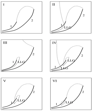
2.1 Six classifications of fluid phase behavior . . . 34

2.2 Method for finding liquid-liquid immiscibility with an UCST . . . 35

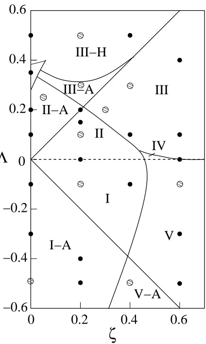
2.3 Parameters for which complete phase diagrams were calculated . . . 36

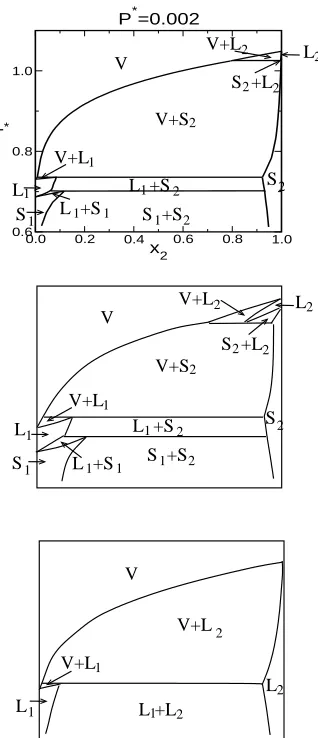
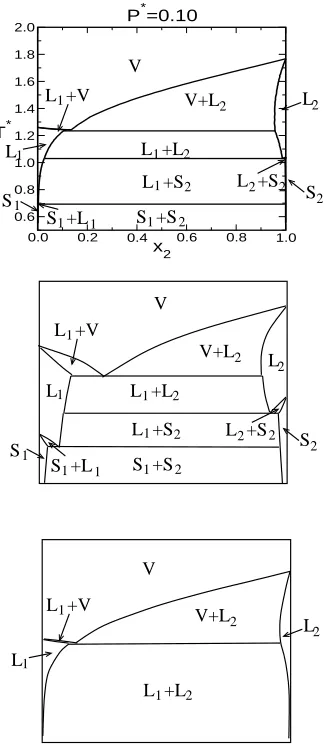
2.4 A series of temperature-composition diagrams at varying pressures with

and "!#%$ . . . 37

2.5 A temperature-composition diagram at a pressure,&(')*+, with* and

-"!./ . . . 38

2.6 A temperature-composition diagram at a pressure,& ' *+, with and

-%$ . . . 39

*,/ and0+/ . . . 40

2.8 A series of temperature-composition diagrams at varying pressures with21

(13)

2.9 A temperature-composition diagram at a pressure, &('45%$ with(63 and

- . . . 42

2.10 A temperature-composition diagram at a pressure, & ' 5%$ with(6 and -3 . . . 43

2.11 A temperature-composition diagram at a pressure, & ' 5*,/ with(6 and -/ . . . 44

2.12 A series of temperature-composition diagrams at varying pressures with78 and "!#%$ . . . 45

2.13 A temperature-composition diagram at a pressure, & ' *+,/ with21 and -"!./ . . . 46

Chapter 3 Solid-Liquid Phase Behavior of Ternary Mixtures 47 3.1 Schematic of ternary Gibbs Duhem integration . . . 65

3.2 Binary phase diagram of component 1 and the solvent at&('.*91, . . . 66

3.3 Binary phase diagram of component 2 and the solvent at&('.*91, . . . 67

3.4 Binary phase diagram of component 1 and component 2 at&:'.*91, . . . 68

3.5 Ternary phase diagram calculated at ; ' $9*+<=& ' *91, and >?A@B C*,+/C<=D ?A@ "$9%$E8+3 . . . 69

3.6 Ternary phase diagram calculated at ; ' $9*+<=& ' *91, and > ?A@ C*,+/C<=D ?A@ "$9%$GF9/ . . . 70

(14)

3.8 Ternary phase diagram calculated at ;'H KF9/C<=&'I *91, and > ?A@

$9J++C<=DL?A@M"$9%$E8+3 . . . 72

3.9 Ternary phase diagram calculated at ; ' $9*+<=& ' *91, and > ?A@

$9J++C<=D ?A@ "$9%$E8+3 . . . 73

3.10 Ternary phase diagram calculated at ; ' $9+/C<=& ' *91, and > ?A@

$9J++C<=D ?A@ "$9%$E8+3 . . . 74

3.11 Ternary phase diagram calculated at ;'H $93+/C<=&'I *91, and > ?A@

$9J++C<=DL?A@M"$9%$E8+3 . . . 75

3.12 Ternary phase diagram calculated at ; ' $93+JC<=& ' *91, and >?A@B

$9J++C<=D ?A@

"$9%$E8+3 . . . 76

Chapter 4 Future Work 77

Appendix A Global phase diagram for monomer/dimer mixtures 82

A.1 Comparison of GFD equation of state to molecular dynamics simulation results

for mixtures of monomers and dimers at > @N@EO > ?N? P/C<E$9* and $9/ , equal

segment diameters and equal volume fractionsQ ?NRC? SQ @TR+@ of the two species. 117

for mixtures of monomers and dimers at>U@N@ O >U?N?VW$9/ andQX@YZ%$+$+$9<=3+3+3C<

and8+8,F and equal segment diameters. . . 118

for mixtures of monomers and 8-mers at > @N@GO > ?N? [/C<E$9*< and $9/ , equal

(15)

A.4 Six classifications of phase behavior . . . 120

A.5 Schematic of a parametrized plot of\]? vs. \L@ . . . 121

A.6 The global phase diagram predicted by the Generalized Flory Dimer theory for

a mixture of square-well monomer and dimers. . . 122

A.7 A schematic of the global phase diagram predicted by the van der Waals equation

of state for a mixture of equal-sized molecules as calculated by van Konynenburg

and Scott . . . 123

(16)

C

HAPTER

1 I

NTRODUCTION

Knowledge of the equilibria between solids and fluids is of vital importance in designing

in-dustrial processes based on crystallization, including separations, purification, concentration,

solidification, and analysis. Crystallization is widely used in the pharmaceutical industry for

product recovery because it yields high purity products with a relatively low energy expenditure

compared to distillation or other common methods of separation. Crystallization has economic

benefits over distillation for components with melting points near ambient conditions because

of its lower energy requirements. The lower operating temperatures typically used in

crystal-lization processes are also important when separating components that would decompose at the

temperatures necessary for distillation?

. Crystallization is also used in the desalination and

de-contamination of wastewater streams@

.

One area of crystallization that is of particular interest to us is chiral drug separation. For

chiral drugs, crystallization is the only feasible means of separation. Chiral drugs are normally

produced as a mixture of two racemates. In general, one of the racemates is the active ingredient;

the other is either inactive or has some unwanted activity. While it desirable to separate the

race-mates, this can not be done through standard techniques because the racemates have identical

(17)

crystallization techniques, which are also known as classical resolution^ . The two racemates are

first reacted with a chiral resolving agent, forming a pair of diastereomers that are chemically

identical but have different physical properties. The diastereomers are then separated using

frac-tional crystallization, taking advantage of the now differing solubilities of the two components.

As of yet the design of a diastereomeric separation process is more an art than a science and we

hope that this research will provide useful insights into the underlying phenomena.

A prerequisite to efficient use of crystallization is knowledge of the solid-liquid phase

equi-libria of the components to be separated. The solid-liquid phase diagram for a mixture has many

uses in the design of a fractional crystallization process. It can be used to identify feasible

opera-tion paths given a known feed stream, choose optimal operating condiopera-tions, and solve the related

mass balances in a separation operation_ . Although the solid-liquid phase diagram for a

partic-ular substance or mixture can be obtained by experiment, limited time and resources generally

allow for only a sampling of possible operating conditions for any given system. Theory and

molecular-level simulation make it possible to gain insight into the phase equilibria of whole

classes of mixtures, rather than just one in particular.

One might think that solid-fluid phase equilibria could be obtained from simulation directly

by simply putting a solid and fluid in contact with each other in the simulation box and allowing

them to come to equilibrium. Unfortunately this is not the case because, for reasonably-sized

systems, the breadth of the interface between the two phases makes it impossible to obtain

ac-curate bulk properties` . Even if the simulation box is large enough to overcome this problem,

system equilibration usually takes a long time due to slow mass transfer across the interfacea .

(18)

the Gibbs ensemble the two phases are simulated in separate boxes, each representing one of the

phases in equilibrium. Mechanical and thermal equilibrium between the boxes is maintained by

conducting the simulations at constant pressure and temperature. Chemical equilibrium is

main-tained by randomly attempting to insert particles from one phase into the other. This technique

does not work well for solid-fluid phase equilibria due to the difficulty of inserting a particle

from the liquid phase into the high-density solid phase. Without a sufficient number of these

swap moves, chemical equilibria is not maintained and the method fails.

An alternative for calculating solid-fluid equilibria in single or multicomponent systems is

the Gibbs-Duhem integration technique of Kofkec de . Instead of using a particle swap move to

maintain chemical equilibrium between the phases, an appropriate form of the Clapeyron

equa-tion is integrated to calculate the phase coexistence line. The Gibbs-Duhem integraequa-tion technique

procedure allows one to calculate an entire phase coexistence envelope in one calculation, rather

than in the many individual steps required when using Gibbs ensemble simulations. By

eliminat-ing the particle exchange move, the Gibbs-Duhem technique also makes it possible to calculate

single and multicomponent solid-fluid phase equilibria.

1.1 Overview

This thesis describes research into the fundamentals of solid-fluid phase equilibria by using

molecular simulation to analyze the phase change behavior of one of the simplest of all possible

mixtures, the Lennard-Jones binary mixture. In this section, we provide a short summary of

the remaining chapters of this thesis. All of the chapters are self-contained units complete with

(19)

Chapter 2 explores how the solid phase affects the global phase diagram of mixtures

com-posed of molecules of equal diameter. This was done by calculating “complete” phase diagrams,

that is including solid, liquid, and vapor phases, at 29 sets of Lennard-Jones parameters using

the Gibbs Duhem integration technique. For the systems studied, the well-depth ratio,> @N@GO > ?N? ,

ranged from 1.0 to 4.0 and the ratio of the interspecies well-depth to the Lorentz-Berthelot

mix-ing rule well-depth, f2> ?A@EOg> ?N? > @N@EhAikj ?lm@=n

, ranged from 0.5 to 1.875. By using the same parameter

definitions as Mazur et al. we are able to compare our results to their predictions for the global

phase diagram of Lennard-Jones mixtures. Phase diagrams were calculated for each region of

the global phase diagram, except for the type IV phase behavior region. We found that for

mix-tures in which the two pure components have similar critical temperamix-tures, the solid phase did

not significantly alter the vapor-liquid phase equilibria except at low pressure. For mixtures in

which the two components had greatly dissimilar critical temperatures, the solid phase interfered

with the fluid phase behavior over a greater range of pressures. In those cases, we found that it

was possible for the presence of the solid phase to change the classification of the fluid-phase

phase behavior.

Chapter 3 explores the role of molecular parameters, such as the Lennard-Jones well-depth

and diameter, in the crystallization of ternary mixtures. We investigate a model diastereomeric

mixture composed of Lennard-Jones particles. The two model diastereomer particles have

sim-ilar well-depths (> ?N? oC*+ vs. > @N@ oC*,/ ) and diameters (D ?N? p$9%$E/ vs. D @N@ q$9%$GF9/ ),

while the solvent has a much lower melting point and slightly smaller diameter ((>srtruv$9*+ and

D

rr

w$9*+ ). The cross-species parameters (>G?A@ and DL?A@ ) between the two diastereomers were

(20)

diameter up to the diameter of the large diastereomer resulted in a slight increase of the solubility

of the solid phase. We found that decreasing the interspecies well-depth to less than that of either

of the diastereomers resulted in an immiscibility in the solid phase and consequently a region of

three-phase equilibria (two solid phases and one liquid phase) in the ternary phase diagram. The

effect of temperature was then explored by calculating phase diagrams over a range of

tempera-tures for a given set of cross-species well-depths and molecular diameters. It was found that as

the temperature increases, the size of the three-phase region decreases until it disappears.

For completeness, an earlier study on the global phase diagram of monomer/dimer

mix-tures has been included in Appendix A. This work was defended as part of my Master of Science

research in September, 2001. In that research, we first extended the Generalized Flory Dimer

theory for hard sphere monomer/x -mer mixtures to square-well monomer/x -mer mixtures.

The-oretical predictions for the compressibility factor as a function of volume fraction are compared

to discontinuous molecular dynamic simulation results on monomer/dimer mixtures at well depth

ratios 0.5 - 1.5 and dimer mole fractions 0.111 - 0.667 and on monomers/8-mer mixtures at well

depth ratios 0.5 - 1.5. Agreement between theory and simulation is very good; this is

consis-tent with the performance of the GFD theory for other square-well systems. Next we calculate

the GFD-predicted global phase diagram for square-well monomer/dimer mixtures using a brute

force method. The locus of critical points in the&"!y; plane is calculated for a grid of points

in the 7!S plane, where is a measure of the difference between the monomer and dimer

well depths and is a measure of the strength of the attraction between monomers and dimers.

Initially, the locus of critical points was calculated for 360 points in a square grid between the

(21)

resolution in areas where more detail was needed. The most significant features of the resulting

global phase diagram is the absence of type IV and type VI behaviors. We also found that the

phase diagram is shifted towards the negative and directions when compared to the van der

Waals global phase diagram for equal diameter spherical molecules.

Chapter 2 and 3 and Appendix A have been adapted from the following publications:

Chapter 2 B. C. Attwood and C. K. Hall., “Effect of the Solid Phase on the Global Phase

Behavior of Binary Lennard-Jones Mixtures,” AIChE Journal, (submitted, 2003).

Chapter 3 B. C. Attwood and C. K. Hall., “Monte Carlo Simulations of Ternary Solid-liquid

Phase Equilibria,” AIChE Journal, (in preparation)

Appendix A B. C. Attwood and C. K. Hall., “Global Phase Diagram for Monomer/Dimer

(22)

1.2 References

[1] Cottin, X. , Paras, P. A. , Vega, C. , and Monson, P. A. , Fluid Phase Equil., 117, 114–125

(1996).

[2] Ericsson, B. and Hallmans, B. , Desalination, 105, 115–123 (1996).

[3] Stinson, S. C. , Chem Eng News, 9, 44 (1995).

[4] Takano, K. , Gani, R. , Ishikawa, T. , and Kolar, P. , Fluid Phase Equil., 194-197, 783–803

(2002).

[5] Panagiotopoulos, A. Z. , J Phys-Condens Mat, 12, R25–R52 (2000).

[6] Yan, Q. L. , Liu, H. L. , and Hu, Y. , Macromolecules, 29, 4066–4071 (1996).

[7] Panagiotopolous, A. Z. , Mol. Phys., 61, 813–826 (1987).

[8] Kofke, D. A. , Mol. Phys., 78, 1331–1336 (1993).

(23)

C

HAPTER

2 E

FFECT OF THE

S

OLID

P

HASE ON THE

G

LOBAL

P

HASE

B

EHAVIOR OF

B

INARY

L

ENNARD

-J

ONES

M

IXTURES

2.1 Introduction

Knowledge of the equilibria between solids and fluids is of vital importance in industrial

processes based on crystallization, including separations, purification, concentration,

solidifi-cation, and analysis. Crystallization is widely used in the pharmaceutical industry for product

recovery because it yields high purity products with a relatively low energy expenditure

com-pared to distillation or other common methods of separation. Crystallization is also used in the

desalination and decontamination of wastewater streams ?

, the resolution of racemic mixtures@

,

and the separation and purification of numerous organic and inorganic mixtures^ . A

prereq-uisite to efficient use of crystallization is knowledge of the solid-liquid phase equilibria of the

components to be separated.

The techniques for calculating phase equilibria of a system based on knowledge of its

(24)

of the molecular interaction parameters in order to predict the phase equilibrium for a particular

fluid or mixture. A different approach was taken in the late sixties by van Konynenburg and

Scott_

–

a who chose to examine the phase behavior predicted for a binary mixture obeying the

van der Waals equation of state over the entire range of interaction parameters. Their approach

involved calculating the locus of critical points as a function of composition, pressure, and

tem-perature. The type of phase behavior could then be classified into different types based on the

projection of the locus of critical points onto the& -; plane, as seen in Fig. 2.1.

For their analysis of mixtures of equal-sized components, Scott and van Konynenburg_Uda

considered two dimensionless interaction parameters, and , which were a function of the

attractive interaction parameters z ?N?

<=z @N@

< and z

?A@ between molecules of components 1 and 2,

where { gz @N@ !z ?N? hNOg z @N@Y| z ?N? h and } gz ?N?#| z @N@ !79z ?A@GhNOgz @N@Y| z ?N? h. For equal

sized molecules, is related to the differences in critical temperatures or pressures of the pure

components and is related to the molar heat of mixing at;66 . By determining the locus of

critical points for a range of these parameters, they were able to construct a global phase diagram

which divides the (!- parameter space into regions of similar phase behavior. Their global

phase diagram for the van der Waals equation of state accounts for five of the six types of fluid

phase behavior known to exist in nature. The only type of phase behavior not found by Scott and

van Konynenburg was type VI, which is distinguished from the other types by a region of closed

loop immiscibility. This was an important result because it showed that even though the van der

Waals equation of state is simplistic and quantitatively inaccurate for most fluids, it is able to

predict much of the phase behavior found in nature.

(25)

phase behavior for other equations of state. Furman et al. calculated the global phase behavior for

a regular solution model of a three-component mixture that is nearly equivalent mathematically

to a van der Waals model for binary mixtures with the parameter~ independent of concentration

(implying that the molecules are of equal size) and the parameter z a quadratic function of

compositionb . They found significant agreement between the phase diagram they calculated and

the one calculated by van Konynenburg and Scott for equal diameter molecules. Later Furman

and Griffithsc revisited the global phase diagram for the van der Waals model and discovered a

heretofore unidentified “shield region”, a small region containing several new classes of phase

behavior that had not been pointed out previously by van Konynenburg and Scott.

Mazur and Boshkove

–?N?

investigated the global phase behavior of binary Lennard-Jones

fluid mixtures using a polynomial form for the equation of state that was proposed earlier and

regressed to simulation data by Ree?A@

. This was the first analysis of the phase behavior of

a relatively modern equation of state that included a systematic look at the entire interaction

parameter space. Mazur and Boshkov’s papers revealed that the global phase behavior predicted

for Lennard-Jones fluids is qualitatively similar to that of the van der Waals equation of state,

except that Type VI phase behavior is also predicted. Dieters and Pegg calculated the global

phase diagram for the Redlich-Kwong equation of state?

^ in 1989 and found that for equal-sized

molecules, the global phase diagram predicted by the Redlich-Kwong equation of state is similar

to that found for the van der Waals fluid or the Lennard-Jones fluid. In this case however, no

instances of Type VI behavior were found. As the difference in molecular size was increased,

the topology of the global phase diagram changed considerably, with new sub-classes of phase

behavior being predicted. Kraska and Dieters?

(26)

equation of state a few years later in 1992. For equal-sized molecules the results were again

similar to those for the van der Waals equation of state. For molecules of different size, some

unusual new phase behavior was found involving four-phase states and high density instabilities.

In recent years, a number of investigators?

`

–?

e have calculated closed-loops of immiscibility

for equations of state based on isotropic potentials, a result that continues to be debated in the

literature. Yelash and Kraska?

` found that even a simple equation of state composed of the

Carnahan-Starling repulsion and the van der Waals attraction exhibited several types of

closed-loop phase behavior. One disadvantage of the global phase diagrams found in the literature is

that they are based on equations of state that are only applicable for fluid phases.

In this chapter, we consider how including the possibility of a solid phase influences the

global phase behavior of a binary mixture of equal-diameter Lennard-Jones molecules. We

cal-culate “complete” phase diagrams, that is including solid, vapor, and liquid phases, for 29 sets of

interaction parameters using the Gibbs Duhem integration technique developed by Kofke@N

d

@ ?

.

Since we have used the same interaction parameters as Mazur et al., we are able to compare our

results to their predictions for the global phase diagram of Lennard-Jones mixtures. It is

impor-tant to point out that our goal is not to remap the global phase diagram, since that is not our focus

and is extremely expensive computationally, but instead to sample the behavior in different

re-gions of the global phase diagram. By calculating temperature-composition phase diagrams at a

number of pressures for each set of interaction parameters we are able to see how the solid phase

influences the type of phase behavior exhibited by the fluid phases. That is, we seek to determine

those sets of parameters for which the classification of the fluid phase behavior with the solid

(27)

fluid phase equation of state.

For certain sets of parameters we consider our results in light of the classification scheme

for complete phase diagrams developed by Valyashko@N@

. Valyashko proposed a scheme of twelve

types based on analysis of experimental data and the method of continuous topological

transfor-mation. Valyashko proposed two main groups of complete phase behavior. In group 1 systems, a

continuous three-phase (SLV) curve in P-T-x space connects the triple points of the two

compo-nents. In group 2 systems, the three-phase (SLV) curve is interrupted by the locus of L-V critical

points, resulting in a discontinuity in both of the curves. Further subclasses are determined by

considering the presence and location of the liquid-liquid immiscibility region and the locus of

the three-phase (SLV) coexistence curve.

Highlights of our results are as follows. We find that for mixtures in which the components

have similar critical temperatures, inclusion of the solid phase does not significantly alter the

types of fluid phase equilibria observed. This is because for these mixtures the melting point

of both components is below the boiling point of either component. As such, the solid phase

can only impact the observed vapor-phase behavior at low pressures close to the triple point

of one or both of the components. Since the phase behavior classification scheme is based

mainly on the locus of the vapor-liquid critical points this low pressure interaction does not

alter the classification of these mixtures. However, as the difference in critical temperatures

increases, the solid phase of the component with the higher critical temperature can coexist with

the vapor phase of the component with the lower critical temperature. This results in some

interesting new behavior, such as the formation of a vapor-solid eutectic point. This interference

(28)

fluid-phase equilibria that are necessary in the classification of the type of phase behavior, such

as the presence of liquid-liquid immiscibility at low temperatures. It is seen that in those cases

the solid phase effectively alters the classification of the fluid phase behavior that would be seen

in experiment from what would have been predicted based on a fluid-phase-only equation of

state.

The remainder of this chapter is organized as follows. In Section 2 we briefly review the

Gibbs-Duhem technique for binary mixtures. In Section 3 we present our results and discuss

their significance. Section 4 concludes the chapter with a brief summary.

2.2 Method

2.2.1 Gibbs Duhem integration technique

The Gibbs Duhem integration technique is based upon integrating an appropriate form of

the Clapeyron equation which describes how the field variables vary as a function of each other

at equilibrium. One can calculate the properties of two coexisting phases as a function of almost

any variable of interest. For a mixture of components, the Gibbs-Duhem equation @N

can be

expressed as

#%6

% ?

% 7

|0

.%

!

% ? Q

(2.1)

where

is the pressure, is the compressibility factor,

QL and

are the mole fraction and

fugacity of species, is the residual molar enthalpy,

(29)

Boltzmann’s constant, and

is the fugacity fraction, defined as

L ? (2.2)

For binary mixtures equation 2.1 reduces to the following

.% g ?|

@Eh 7

|0 .%

!

Q @ !

@ @,g $#! @Eh @ (2.3)

sinceQ ? Z$)!Q @ and

? Z$)!

@ .

The Gibbs-Duhem equation can be applied to two phases, and , in equilibrium, by

writing Eq. 2.3 for each of the phases. Since the fugacity, and hence the fugacity fraction, of

each of the components is identical in phases and , we can set the right-hand sides of those

two equations equal to get

|0 #% ! Q @ ! @ @,g $.! @Eh @.7 |0 .% ! Q @ ! @ @9g $#! @Eh @ (2.4)

At this point one has a choice as to which variable to hold constant and which variable to

inte-grate with respect to. In the calculation of temperature-composition diagrams we hold pressure

constant and integrate Eq. 2.4 with respect to the fugacity fraction of component 2. Solving for

,

O

,

@ we get

@ Q @ !¡Q @ g !¢ h @,g $.! @h (2.5)

By starting with values of

and

@ at a known equilibrium point, we can calculate

as a

function of

(30)

an initial value for the integrand is needed. In general, we start the integration at one of the

pure components, i.e.

@4v or $ . Because the right-hand side of Eq. 2.5 is undefined at either

of these conditions, we obtain its value by calculating its limit as

@¤£ ¦¥+§)$ . Assuming the

mixtures to be ideal as

@#£ , the following approximations are made

@)Q@¨(@ (2.6) ? ª© ? (2.7) where ©

? is the fugacity of pure component 1; these approximations are based on Henry’s law

and the Lewis Randall rule, respectively. Thus we can write

@¬« « «® °¯²±E³ ´ µ ®9¶ ! ¯¬±E³ ´ µ ®s¶ !y (2.8)

The quantity ª·

?

O ¨:@ can be evaluated during an NPT simulation (at the boiling temperature

of pure component 1 for the desired pressure) on pure component 1 by performing trial identity

switches of randomly chosen atoms. The value of

·

?

O ¨ @ can then be calculated from

· ? ¨ @ Z¸º¹U»¼ gk½u¾²¿ÁÀXÃÂ ÁÄ

O9 ; hNÅmÆÇXÈ (2.9)

where¸ Å denotes the ensemble average and¾]¿ÁÀXÃÂ ÁÄ

is the potential energy change upon switching

particle identities. The values of g ·

?

O ¨ @Gh and

g

·

?

O ¨ @Gh

can be calculated by conducting a

simulation at the density of the and phases respectively. If we are starting the integration

for -É

(31)

the initial value of the integrand. In either case, the values of the compositions and enthalpies in

Eq. 2.5 will either be known from a prior Gibbs-Duhem integration or can be calculated by an

NPT

@ simulation at the desired temperature, pressure, and fugacity fraction.

Once the initial condition is calculated, the integration is carried out using a standard

predictor-corrector algorithm. A step,½

@ , in the fugacity fraction value is taken and the

predic-tor formula is used to find the new value for the inverse temperature, i.e.

?

|0Ê ®

ÌË ® ®

@

,

@ (2.10)

A separate semigrand ensemble (constant NPT

@ ) Monte Carlo simulation is then performed

for each of the coexisting phases to evaluate the enthalpy and composition at the new fugacity

fraction and temperature. After the simulations have equilibrated, the integrand is recalculated,

the corrector formula is applied to find the “corrected” inverse temperature, and more simulations

are performed at the new value for the temperature. This corrector step is repeated until the

inverse temperature converges to its final value. A production run of simulations is then carried

out to calculate the final values for the enthalpies and compositions of the coexisting phases.

These values are then used in the predictor formula to calculate the inverse temperature at the

next value of the fugacity fraction. Continuing this process we can calculate the entire phase

coexistence envelope, starting at phase equilibrium for either of the pure components.

For certain sets of parameters, there is a range of pressures for which two two-phase

co-existence envelopes, e.g. vapor-liquid and liquid-solid, overlap over a range of temperatures

resulting in three-phase equilibria, e.g. vapor-liquid-solid coexistence, at the point of

(32)

for which the envelopes overlap. The solid-vapor coexistence envelope is calculated by

conduct-ing a Gibbs Duhem integration startconduct-ing at the values of temperature and

@ at the point of overlap

of the vapor-liquid and liquid-solid coexistence envelopes. The solid and vapor phases at that

temperature are used as the initial coexisting phases to start the integration. This procedure is

explained in greater detail in a paper by Lamm and Hall@ ^ .

A different approach is needed to calculate low-temperature liquid-liquid immiscibility with

an UCST, as would be found in type II phase behavior at higher pressures, because those curves

do not originate at either of the pure components. One way to calculate an initial point for

starting the integration would be to use Gibb’s ensemble simulation to calculate the properties of

the coexisting liquids at one temperature. We have developed an alternative approach that makes

use of the Gibb Duhem integration technique, as illustrated in Fig. 2.2 for the systemÍB

and ÎÏ%$GF9/ . Our approach starts by calculating a temperature-composition diagram at a

pressure (&'ÐÎ*91 ) lower than the desired pressure, where there is three-phase coexistence

(Fig. 2.2(a)). We then choose a temperature (; ' oÑ+Ñ ) below the three-phase coexistence

temperature at which two liquids are in equilibrium (solid circles on Fig. 2.2(a)). After that a

Gibbs Duhem pressure integration can be conducted at constant temperature (; ' vÑ+Ñ ) up to

the pressure (& ' I*,/ ) of interest (open circles Fig. 2.2(b)) using the following form of the

Clapeyron equation

& '

@

Q

@

!¡Q

@

gÁ

!

h

@+g $.!

@Eh

(2.11)

The resulting two coexisting liquid state points can then be used as initial conditions (open circles

(33)

2.2.2 Simulations

As mentioned previously, semigrand ensemble Monte Carlo (NPT

@ ) simulations are used

to evaluate the properties of the coexisting phases during the integration of the Gibbs-Duhem

equation. In this section, we briefly describe how these simulations are conducted.

There are three types of moves in the semigrand ensemble: particle displacement, volume

change, and identity exchange. The particle displacement and volume change moves are carried

out in the same manner as in isothermal-isobaric (NPT) simulations. The identity exchange move

involves choosing a random molecule in the system and switching its identity. The change in the

configurational energy of the system caused by the identity change is then evaluated. The overall

acceptance probability,Ò , for these moves is

ÒvÓ:Ô

fÃ$9<N¹U»C¼ g !

g¾¦Õ×ÖºØ*ÙmÚ ! ¾¦ÛNÚ2Ü,h !

& gÁÝVÕ×ÖºØ*ÙmÚ ! ÝYÛNÚ2Ü,hª| % Ý

Õ×ÖºØ*ÙmÚ

Þ

ÛNÚ2Ü

|

%

Â àßâá

·

áã

hAi (2.12)

where ¾

Õ×ÖºØ*ÙmÚ and

¾

ÛNÚ2Ü are the configurational energies,

Ý

Õ×ÖºØ*ÙmÚ and

Ý

ÛNÚ2Ü are the volumes of the

trial and existing states respectively, is the total number of molecules, and

Â

àßâá and

·

áKã refer

to the fugacity fractions of the trial and existing identities of the molecule during the identity

exchange moves. At each step, the type of move is randomly chosen with a weighting such

that for every volume change move there are 20 particle displacements and 20 identity exchange

moves. After an appropriate number of equilibrium moves, running averages of the composition

and enthalpy (as calculated by v ¾)O | & ÝäO ) are calculated for use in evaluating the

integrand in the Gibbs Duhem technique.

Other details of the simulation are as follows. Prior theoretical calculations@

(34)

simulations@

` have shown that by choosing diameter ratiosJ+/(åæD ?N? O D @N@ å6$9* we can assume

that the most stable configuration for the solid phase will be that of a substitutionally disordered

fcc lattice. By using an fcc lattice as an initial configuration for the solid phase, an fcc lattice will

be maintained in the solid phase throughout the simulation without any additional constraints on

the simulation. The simulations are performed on a system of 500 molecules in a cubic box with

periodic boundary conditions. The molecules interact via the Lennard-Jones potential

ç

*è gºéth

S1t>N*è

¯

D*è

é

¶

?A@

!

¯

Dê*è

é

¶

a

(2.13)

where ç

*è is the potential energy of the interaction between atoms and ë , é is the distance

between atoms and ë , >T2è is the Lennard-Jones well-depth, and DÌ*è is the Lennard-Jones

di-ameter. The potential interactions are truncated at half the box length and standard long-range

corrections@

a are applied to the potential energy and pressure calculations.

2.3 Results and Discussion

We have calculated complete phase diagrams at conditions indicated by the circles on the

Mazur et al. global phase diagram shown in Fig. 2.3. The small dots indicate sets of parameters

at which complete phase diagrams have been calculated for at least one pressure and the larger

dots indicate sets of parameters at which complete phase diagrams have been calculated at more

than one pressure. We have not calculated the phase behavior in region IV because that region

is very small. In addition, it is difficult to be sure that a chosen set of parameters will lie within

(35)

equation of state. In each of the phase diagrams presented here, the upper row of diagrams show

the phase behavior calculated using the Gibbs Duhem technique for the fluid and solid phases,

the middle row is a schematic of the upper row of diagrams presented when necessary, and the

bottom row shows the phase behavior calculated when considering only the fluid phases. The

fluid-phase-only diagrams were calculated by simply omitting the calculation of the solid-fluid

phase coexistence. In this way we are able to calculate metastable fluid phase equilibria below

the freezing point of the mixtures. In the fluid-phase-only diagrams, the dotted lines indicate

portions of the diagram whose presence is inferred rather than calculated. In these cases the

fluid phase was sufficiently unstable compared to the solid phase that it spontaneously solidified

during the simulation. Table 2.1 lists the temperature and compositions of the coexisting phases

for each of the three-phase coexistence lines found in Figs. 2.4-2.13. In both the figures and the

table,&')ì&YDª^ ?N?

O > ?N? and;M')ì ; O > ?N? .

Fig. 2.4 shows a series of temperature-composition phase diagrams at decreasing pressures

for 0Ï and Îí!.%$ , which is in the type I region on the Mazur et al. global phase

diagram. In terms of the fluid-phase-only phase behavior classification, Type I phase behavior

is characterized by a single vapor-liquid phase coexistence envelope terminated at either end by

the pure component boiling points at the pressure of interest. We find that at high pressures (e.g.

&':I*,/ , Fig. 2.4(a)), the solid does not affect the fluid phase equilibria because the

vapor-liquid phase coexistence envelope occurs at a significantly higher temperature than the

solid-liquid phase coexistence envelope. At intermediate pressures (e.g.&:'.*+,/ Fig. 2.4(b) ) , the

solid-liquid phase coexistence envelope intersects with the descending vapor-liquid phase

(36)

re-gions of vapor-liquid, liquid-solid, and vapor-solid phase coexistence. Between these two

three-phase lines lies a range of temperatures at which there is coexistence between a solid three-phase and

a vapor phase. As the pressure decreases further, the range of temperatures at which vapor-solid

equilibria occurs broadens until the triple point pressure of pure component 2 (&

'

*+$E8+/ ) is

reached. Below this there is no longer solid-liquid and vapor-liquid equilibria for pure component

2, but only solid-vapor equilibria. At low pressures (e.g. &:'îH*+$U1t+/ , Fig. 2.4(c) ), which

is below the triple point pressure of component 2, the phase coexistence is predominantly

solid-vapor. Without including the possibility of a solid phase, we would be unable to see any of the

three phase (SLV) coexistence curves in region I. The complete phase behavior can be classified

as type 1a according to Valyashko’s scheme based on examining the temperature-composition

phase diagrams shown in Fig. 2.4. An experimental system which has similar complete phase

behavior is silver nitrate + water@ b .

Fig. 2.5 shows a temperature-composition phase diagram at &('îB*+, forï* and

6ð!./ , which is in the type I-A region on the Mazur et al. global phase diagram. Because

the mixture is symmetric (zX?N?¤wz@N@ ) the diagram is symmetric about QL@ñw/ . In terms of

fluid-phase-only phase behavior classification, Type I-A differs from Type I in that Type I-A

exhibits an azeotrope in the vapor-liquid phase coexistence envelope. When including the solid

phase, we find that there is an azeotrope in the solid-liquid phase coexistence envelope as well.

Because of the presence of the azeotrope there are two regions of vapor-solid phase coexistence,

in contrast with the single region of vapor-solid phase coexistence seen in Figs. 2.4(a)and 2.4(b).

Fig. 2.6 shows a temperature-composition phase diagram at &

'

(37)

fluid-phase-only phase behavior classification, the fluid phase equilibria is similar to that of type

I except that type II has low temperature liquid-liquid immiscibility. The pressure& ' Z*+,

is just above the triple point of component 2. Two three-phase coexistence lines (VL@ S@ and

VL? S@ ) separate regions of liquid and liquid-solid coexistence from a region of

vapor-solid coexistence, while one three-phase coexistence line (L? S? S@ ) separates regions of

liquid-solid coexistence from the region of liquid-solid-liquid-solid coexistence. It can be seen that for this set of

pa-rameters and at this particular pressure and temperature, liquid-liquid immiscibility is metastable

compared to the liquid-solid and solid-solid phase equilibria since liquid-liquid immiscibility is

present in the fluid-phase-only diagram, but not in the complete phase diagram.

Fig. 2.7 shows a series of temperature-composition phase diagrams at decreasing pressures

forò*,/ and0+/ , which is in the type II-A region on the Mazur et al. global phase

di-agram. In terms of the fluid-phase-only phase behavior classification, Type II-A phase behavior

is the same as type II with the addition of an azeotrope in the vapor-liquid coexistence curves.

At the highest pressure (& ' H*,J , Fig. 2.7(a)) we can see that below; ' óKF9/+/ the

liquid-liquid immiscibility becomes less stable than liquid-liquid-solid phase coexistence. The interference

between the solid phase and liquid phases results in the formation of two three-phase

coexis-tence lines (L? L@ S@ ) and (S? L? S@ ) separating liquid-liquid, liquid-solid, and solid-solid phase

coexistence. We are unable to calculate the liquid-liquid immiscibility curve all the way up to

the UCST because as the critical point is approached, density fluctuations cause the simulation to

become unstable. The dashed line indicates where we expect the curve would be, approximately.

The liquid-liquid coexistence curves in this case were calculated by the method described in

(38)

envelope interferes with the liquid-liquid coexistence curves and a third three-phase line (L? VL@ )

is produced. As the pressure decreases further the L? VL@ line decreases in temperature and the

L? L@ S@ increases in temperature until they eventually coincide to form a four phase (L? VL@ S@ )

line at one value of the pressure (the quadruple point). We have not located the quadruple point

directly because this involves guessing the exact temperature at which it occurs. (An alternative

approach would be to conduct two Gibbs Duhem integrations along the two three-phase lines

(L? VL@ and L? L@ S@ ) to find the pressure at which they merge. This is beyond the scope of this

paper.) At the lowest pressure shown (& ' ð*+$+$E8 , Fig. 2.7(c)) , which is below the triple

point of component 2, there are two three-phase lines (S? L? V) and (S? VS@ ). The liquid-liquid

immiscibility has been completely obscured by the presence of the solid phase. In addition, a

solid-vapor eutectic point, a vapor in equilibrium with two solid phases, has been formed. The

interesting phenomena here are the changes in the three-phase lines as the pressure decreases and

the formation of a vapor-solid eutectic point, neither of which would be seen without including

the possibility of the solid phase. The complete phase behavior can most closely be classified

as type 1b

according to Valyashko’s scheme based on examining the temperature-composition

phase diagrams shown in Fig. 2.7. Based on the series of phase diagrams shown in Fig. 2.7, the

experimental system ethane + x -tetrasocane exhibits the most similar phase behavior although

there is no azeotrope in the vapor-liquid phase equilibria @ c .

Fig 2.8 shows a series of temperature-composition phase diagrams at decreasing pressures

for 0Ï21 and }Ï3 , which is in the type III region on the Mazur et al. global phase

diagram. In terms of the fluid-phase-only phase behavior classification, Type III phase behavior

(39)

component critical point to the other. At the highest pressure (&:':ô%$E/ , Fig. 2.8(a)), which

is above the critical pressure of pure component one, we see that the interference of the solid

phase with the vapor-liquid equilibria results in two three-phase coexistence lines (VL@ S@ and

VS? S@ ) separating regions of vapor-liquid, vapor-solid, and solid-solid phase coexistence. At

the two lower pressures (& ' 5*,/ , Fig. 2.8(b) and& ' v*+,/ , Fig. 2.7(c)), which are below

the critical pressure of component 2, a third three-phase coexistence line (VL? S@ ) is formed and

liquid-solid phase coexistence appears. One feature of type III phase behavior that we do not see

in this series of graphs is liquid-liquid immiscibility. Because the melting point of component

two is above the boiling point of component one, we find liquid-solid and solid-solid phase

coexistence occurring in the region where we would have expected liquid-liquid immiscibility.

We did find a small set of parameter sets in the type III region where liquid-liquid immiscibility

was not completely hidden by the liquid-solid and solid-solid phase equilibria. Figure 2.9 is

one such set of parameters, withB3 and vB . It can be seen that for a narrow range

of temperature there are two liquids in equilibrium with each other. We could not find a set of

parameters in the type III region in which the UCST of the liquid-liquid immiscibility was stable

with respect to the solid-liquid and solid-solid phase equilibria. The complete phase behavior

can most closely be classified as type 2a according to Valyashko’s scheme based on examining

the temperature-composition phase diagrams shown in Fig. 2.8. An experimental system which

has similar complete phase behavior is sodium sulfate and water@ b .

Fig. 2.10 shows a temperature-composition phase diagram at &:'õB%$ forï and

5H3 , which is in the type III-A region on the Mazur et al. global phase diagram. In terms

(40)

from type III by the presence of an azeotrope in the vapor-liquid phase diagram at high

pres-sures. It can be seen in Fig. 2.10, that the interference of the solid phase with the vapor-liquid

equilibrium results in the formation of two additional three-phase coexistence lines (L? L@ S@ and

S? L? S@ ) separating regions of liquid-liquid, liquid-solid, and solid-solid phase equilibria.

Al-though we investigated the phase behavior at a number of different pressures, we never located a

UCST for the liquid-liquid immiscibility, which indicates that this set of parameters may actually

be in the Type III-H region.

Fig. 2.11 shows a temperature-composition phase diagram at & ' B*,/ forï and

5H/ , which is in the type III-H region on the Mazur et al. global phase diagram. In terms

of the fluid-phase-only phase behavior classification, Type III-H phase behavior is distinguished

from type III by the presence of a heteroazeotrope in the vapor-liquid phase diagram, that is a

vapor-liquid eutectic. It differs from Type III-A in the following way. While Type III-A also

has a heteroazeotrope at low pressure, as the pressure is increased the vapor-liquid equilibria

separates from the liquid-liquid equilibria and the heteroazeotrope is replaced by an azeotrope.

In Type III-H phase equilibria, the heteroazeotrope is not replaced by an azeotrope at any

pres-sure. In this figure we can see that the increased value of compared to that in Fig. 2.10, (i.e.

decreased attractions between the two components) has caused the two components to become

more immiscible.

Fig 2.12 shows a series of temperature-composition phase diagrams at decreasing pressures

for ö8 and ô[!.%$ , which is in the type V region on the Mazur et al. global phase

diagram. In terms of the fluid-phase-only phase behavior classification, the unique feature of

(41)

vapor-liquid coexistence envelope, as depicted by the dashed lines in the bottom ;"!{Q diagram at

& ' ÷%$E/ (Fig. 2.12(a)). However, we found that interference by the solid obscured the region

in which this liquid-liquid immiscibility is supposed to occur. The consequence of this is that

although the equation of state might predict that this system should exhibit type V phase behavior,

experimentally it would appear to behave more like a type I mixture. As indicated in the

fluid-phase-only diagrams by the dashed line, we were unable to calculate the complete fluid phase

coexistence envelopes at the two lowest pressures. This occurred because the coexisting vapor

and liquid phases became so unstable as the vapor-solid coexistence region was entered during

our simulations, that the liquid phase spontaneously crystallized resulting in coexisting vapor and

solid phases. This prevented us from confirming the existence of the liquid-liquid immiscibility

expected for type V phase behavior. Similar attempts to find the LCST atò8 and0"!#3

or Iq!./ were also unsuccessful. The complete phase behavior can be classified as type

2a according to Valyashko’s scheme based on examining the temperature-composition phase

diagrams shown in Fig. 2.12. An experimental example of a system which exhibits similar phase

behavior is carbon dioxide +x -tetrasocane

@

e .

Fig. 2.13 shows a temperature-composition phase diagram at & ' "*+,/ for¤v21 and

0"!./ , which is in the type V-A region on the Mazur et al. global phase diagram. In terms of

the fluid-phase-only phase behavior classification, Type V-A phase behavior is similar to Type V

phase behavior with the additional feature of an azeotrope in the vapor-liquid phase coexistence

envelope. In Fig. 2.13, it can be seen that there is an azeotrope in both the vapor-liquid and

solid-liquid phase coexistence envelopes. Furthermore, we see that the interference of the solid phase

(42)

separating regions of vapor-liquid, vapor-solid, and liquid-solid phase coexistence.

2.4 Conclusions

Our general conclusions are that for mixtures in which the components have similar critical

temperatures, i.e. yÉó3 , inclusion of the solid phase does not alter how the phase behavior

of the mixture would be classified based solely on the fluid phase behavior. This is because the

classification scheme is based primarily on the locus of gas phase critical points. For values of

close to zero, the influence of the solid phase is only felt at temperatures and pressures well below

the critical point of either species, which means that it does not alter the topology of the locus

of critical points. This is seen to be especially true in regions I and II. For mixtures in which the

components have greatly dissimilar critical temperatures, i.e. ñøS21 , the fluid phase behavior

type may be different from what is expected because the solid phase for the component with the

higher critical point can exist in equilibrium with supercritical phases of the other component.

When this happens, the coexistence between a vapor rich in one species and a solid rich in the

other species can alter the topology of the locus of vapor-liquid critical points. This was seen in

the figures presented for region V.

2.5 Summary

The Gibbs Duhem integration technique was used to calculate composition-temperature

phase diagrams at 29 different points on the global phase diagram for binary mixtures of

Lennard-Jones molecules. We presented phase diagrams calculated in each region of the global

(43)

diagram calculated by Mazur et al. using a polynomial equation of state for binary mixtures

of Lennard-Jones molecules. We found that for mixtures of components with similar critical

temperatures, i.e. ùÉï3 , the phase behavior was essentially the same as in the

fluid-phase-only case. For mixtures in which the components had greatly dissimilar critical temperatures,

¡ø"21 , interaction between the vapor and solid phases could significantly alter the fluid-only

phase behavior. This was manifested in interesting types of solid-fluid phase behavior, such as a

vapor-solid eutectic point, that is - a vapor in equilibrium with two immiscible solids. We found

that a mixture that would be expected to have type V phase behavior according to a fluid-phase

equation of state might experimentally exhibit type I phase behavior. This is because the phase

behavior features unique to type V phase behavior occur below the freezing point of the

mix-tures. We also found that while the Gibbs Duhem integration technique does make it possible

to calculate metastable phase behavior below the freezing point of the mixtures, the calculations

(44)

2.6 References

[1] Ericsson, B. and Hallmans, B. , Desalination, 105, 115–123 (1996).

[2] Schroer, J. W. , Wibowo, C. , and Ng, K. M. , AICHE J, 47, 369–387 (2001).

[3] Kramer, H. J. M. and Jansens, P. J. , Chem. Eng. Tech., 26, 247–255 (2030).

[4] van Konynenburg, P. H. . Critical Lines and Phase Equilibria in Binary Mixtures. PhD

thesis, University of California, Los Angeles, (1968).

[5] van Konynenburg, P. H. and Scott, R. L. , Discuss Faraday Soc., 49, 87 (1970).

[6] van Konynenburg, P. H. and Scott, R. L. , Philos. Trans. R. Soc. London, Ser. A, 298, 495–

540 (1980).

[7] Furman, D. , Dattagupta, S. , and Griffiths, R. B. , Phys. Rev. B, 15, 441–464 (1977).

[8] Furman, D. and Griffiths, R. B. , Phys. Rev. A, 17, 1139–1148 (1978).

[9] Mazur, V. A. , Boshkov, L. Z. , and Fedorov, V. B. , Dokl. Akad. Nauk SSSR, 282, 137–140

(1985).

[10] Boshkov, L. Z. and Mazur, V. A. , Russ. J. Phys., 60, 16–20 (1986).

[11] Boshkov, L. Z. , Dokl. Akad. Nauk SSSR, 294, 901–905 (1987).

[12] Ree, F. H. , J. Chem. Phys., 73, 5401–5403 (1980).

[13] Deiters, U. K. and Pegg, I. L. , J. Chem. Phys., 90, 6632–6641 (1989).

(45)

[15] Yelash, L. V. and Kraska, T. , Ber. Bunsenges. Phys. Chem., 102, 213–223 (1998).

[16] Yelash, L. V. and Kraska, T. , Phys. Che. Chem. Phys., 1, 307–311 (1999).

[17] Yelash, L. V. , Kraska, T. , and Deiters, U. K. , J. Chem. Phys., 110, 3079–3084 (1999).

[18] Scott, R. L. , Phys. Che. Chem. Phys., 1, 4225–4231 (1999).

[19] Wang, J.-L. , Wu, G.-W. , and Sadus, R. J. , Mol. Phys., 98, 715–723 (2000).

[20] Kofke, D. A. , Mol. Phys., 78, 1331–1336 (1993).

[21] Kofke, D. A. , J. Chem. Phys., 98, 4149–4162 (1993).

[22] Valyashko, V. M. , Z. Phys. Chemie, 267, 481–493 (1986).

[23] Lamm, M. H. and Hall, C. , AICHE J, 47, 1664–1675 (2001).

[24] Cottin, X. . A Theoretical Study of the Thermodynamics of Solid Solutions and Solid-Liquid

Phase Equilibria. PhD thesis, University of Massachuesetts, (1996).

[25] Kranendonk, W. G. T. and Frenkel, D. , Mol. Phys., 72, 679–697 (1991).

[26] Allen, M. P. and Tildesley, D. J. , Computer Simulation of Liquids. Oxford Science

Publi-cations, (1997).

[27] Findlay, A. , The Phase Rule. Dover Publications, Inc., 9th edition, (1951).

[28] Peters, C. J. , Lichtenthaler, R. N. , and de Swaan Arons, J. , Fluid Phase Equil., 29, 495–

504 (1986).

(46)

>=@N@ >U?A@ P' T' Phases QX@ Figure

1.500 1.375 0.005 0.873 V-L@ -S 0.014, 0.364, 0.462 Fig. 2.4(b)

0.919 V-L? -S 0.045, 0.524, 0.595

0.001425 0.715 V-L-S 0.000, 0.037, 0.087 Fig. 2.4(c) 1.000 1.500 0.002 0.740 V-L-S 0.000, 0.062, 0.108 Fig. 2.5

0.852 V-L-S 0.052, 0.356, 0.375

1.500 1.125 0.002 0.701 L? -S? -S@ 0.060, 0.117, 0.932 Fig. 2.6

0.736 V-L? -S@ 0.008, 0.088, 0.924

1.025 V-L@ -S@ 0.803, 0.997, 0.999

1.105 0.789 0.08 0.690 S? -L? -S@ 0.005, 0.012, 0.995 Fig. 2.7(a)

0.760 L? -L@ -S@ 0.024, 0.982, 0.994

0.01 0.685 S? -L? -S@ 0.005, 0.011, 0.996 Fig. 2.7(b)

0.755 L? -L@ -S@ 0.024, 0.982, 0.994

0.841 L? -V-L@ 0.049, 0.329, 0.963

0.0016 0.673 S? -V-S@ 0.007, 0.246, 0.997 Fig. 2.7(c)

0.686 S? -L? -V 0.001, 0.002, 0.058

2.333 1.167 0.15 0.700 V-S? -S@ 0.002, 0.004, 0.999 Fig. 2.8(a)

1.607 V-L@ -S@ 0.033, 0.990, 0.998

0.05 0.689 L? -S? -S@ 0.002, 0.004, 1.000 Fig. 2.8(b)

1.122 V-L? -S@ 0.003, 0.008, 1.000

1.603 V-L@ -S@ 0.062, 0.996, 0.999

0.005 0.687 L? -S? -S@ 0.002, 0.004, 1.000 Fig. 2.8(c)

0.838 V-L? -S@ 0.002, 0.007, 1.000

1.594 V-L@ -S@ 0.479, 0.998, 1.000

1.857 1.143 0.10 0.688 V-S? -S@ S 0.002, 0.004, 1.000 Fig. 2.9

1.257 L? -Lú -S@ 0.093, 0.942, 0.988

1.283 V-L? -L@ 0.043, 0.097, 0.932

1.500 0.875 0.10 0.692 S? -L-S 0.002, 0.003, 1.000 Fig. 2.10

1.030 L? -L@ -S@ 0.027, 0.986, 0.997

1.243 L? -V-L@ 0.116, 0.135, 0.956

1.500 0.625 0.05 0.691 S? -L? -S@ 0.000, 0.001, 1.000 Fig. 2.11

1.033 L? -L@ -S@ 0.005, 0.999, 1.000

1.104 L? -V-L@ 0.006, 0.066, 0.998

4.000 2.750 0.15 2.614 V-L@ -S 0.036, 0.879, 0.956 Fig. 2.12(a)

0.05 1.149 V-L? -S 0.000, 0.002, 0.469 Fig. 2.12(b)

2.697 V-L@ -S 0.088, 0.952, 0.984

0.005 0.808 V-L? -S 0.000, 0.003, 0.214 Fig. 2.12(c)

2.746 V-L@ -S 0.802, 0.999, 1.000

2.333 2.500 0.005 0.806 V-L? -S 0.000, 0.021, 0.126 Fig. 2.13

1.572 V-L@ -S 0.170, 0.684, 0.717

(47)

2.7 Figures

Page

2.1 Six classifications of fluid phase behavior . . . 34

2.2 Method for finding liquid-liquid immiscibility with an UCST . . . 35

2.3 Parameters for which complete phase diagrams were calculated . . . 36

and "!#%$ . . . 37

2.5 A temperature-composition diagram at a pressure,&(')*+, with* and

-"!./ . . . 38

2.6 A temperature-composition diagram at a pressure,& ' *+, with and

-%$ . . . 39

*,/ and0+/ . . . 40

and 3 . . . 41

2.9 A temperature-composition diagram at a pressure, & ' 5%$ with(63 and

- . . . 42

2.10 A temperature-composition diagram at a pressure, &

'

5%$ with(6 and -3 . . . 43

2.11 A temperature-composition diagram at a pressure, &('45*,/ with(6 and

(48)

and "!#%$ . . . 45

2.13 A temperature-composition diagram at a pressure, & ' *+,/ with21 and

(49)

II

III

IV

V

VI

1

2 ₂

2

1

2 2

1 2

1 I

1

LLG LLG

LLG

(50)

L1

L₂ L₂

0.0 0.2 0.4 0.6 0.8 1.0

x₂

1.0 1.2 1.4 1.6

T*

P*=0.04

0.0 0.2 0.4 0.6 0.8 1.0

x₂

0.02 0.03 0.04 0.05 0.06 0.07

P*

T*=0.99

0.0 0.2 0.4 0.6 0.8 1.0

x₂

1.0 1.2 1.4 1.6

T*

P*=0.05

V+L

L +L _{L +L}

L +L

L L

V+L V+L

V V

1 2

L

1 ₁ ₂ 2

2 1

1 2

(a) (b) (c)

(51)

ûû ûûü

ü

ýý ýý þþ þþ ÿÿ

ÿÿ

Monte Carlo Simulation of Solid-Fluid Phase Equilibria in Binary and Ternary Mixtures

and Ternary Mixtures

Table of Contents

List of Tables

List of Figures

C

HAPTER

1

I

NTRODUCTION

1.1

Overview

1.2

References

C

HAPTER

2

E

FFECT OF THE

S

OLID

P

HASE ON THE

G

LOBAL

P

HASE

B

EHAVIOR OF

B

INARY

L

ENNARD

-J

ONES

M

IXTURES

2.1

Introduction

2.2

Method

2.3

Results and Discussion

2.4

Conclusions

2.5

Summary

2.6

References

2.7

Figures

II

III

IV

V

VI

V−A

I−A

III−H

II

I

V

II−A

III−A

0

0.2

0.4

0.6

−0.6

−0.4

−0.2

0

0.2

0.4

0.6

Λ

ζ

IV

III