Ensemble methods for top-N recommendation

(1)

A Thesis

Submitted to the Faculty of

Purdue University by

Ziwei Fan

In Partial Fulfillment of the Requirements for the Degree

of

Master of Science

May 2018 Purdue University Indianapolis, Indiana

(2)

THE PURDUE UNIVERSITY GRADUATE SCHOOL

STATEMENT OF COMMITTEE APPROVAL

Dr. Xia Ning, Chair

Department of Computer and Information Science Dr. Mohammad Al Hasan

Department of Computer and Information Science Dr. Murat Dundar

Department of Computer and Information Science

Approved by:

Dr. Shiaofen Fang

(3)

(4)

ACKNOWLEDGMENTS

I want to express my sincere gratitude to my advisor Dr. Xia Ning for her con-tinuous support in my master studies. Her guidance helped me in all the time of research and writing of this thesis. I could not have imagined having a better advisor and mentor for my master studies. I also want to thank my thesis committee, Dr. Mohammad Al Hasan and Dr. Murat Dundar for their help in finishing my thesis.

Next, I want to thank all labmates, Wen-hao Chiang, Junfeng Liu, Evan Burgen and Bo Peng for the interesting discussions, for the continuous support , and for the fun we have had in the last two years.

I also want to thank the support and resources provided by IUPUI. I want to thank Nicole Wittlief as well for her support and patience.

Last but not least, I want to thank my parents sincerely for their financial and emotional support. Without their support, I would have never been able to study in IUPUI and finish the thesis.

(5)

TABLE OF CONTENTS

Page

LIST OF TABLES . . . .viii

LIST OF FIGURES . . . ix

ABSTRACT . . . x

1 INTRODUCTION . . . 1

1.1 Thesis Outline. . . 2

2 BACKGROUND OF RECOMMENDER SYSTEMS . . . 3

2.1 Formulations of Recommendation Problems . . . 3

2.1.1 Rating Prediction . . . 4

2.1.2 Top-N Recommendation . . . 4

2.2 Collaborative Filtering Models . . . 4

2.2.1 Neighborhood-Based Collaborative Filtering . . . 5

2.2.2 Model-Based Methods . . . 7

2.3 Related Work of Top-N Recommendation . . . 7

2.3.1 Sparse Linear method (SLIM) . . . 8

2.3.2 Bayesian Personalized Ranking . . . 8

2.3.3 CLiMF: Collaborative Less-is-More Filtering . . . 9

3 IMPROVING INFORMATION RETRIEVAL FROM ELECTRONIC HEALTH RECORDS USING DYNAMIC AND MULTI-COLLABORATIVE FILTER-ING . . . 11

3.1 Introduction . . . 11

3.2 Literature Review . . . 12

3.3 Terminologies, Definitions and Notations . . . 13

3.4 Overview of the Dynamic and Multi-Collaborative Filtering Method – DmCF . . . 14

(6)

Page

3.5.1 Background on Markov Chains . . . 16

3.5.2 First-Order Markov Chain-based Scoring – foMC . . . 16

3.6 Multi-Collaborative Filtering-based Scoring. . . 17

3.6.1 Background on Collaborative Filtering . . . 17

3.6.2 Physician-Patient-Similarity-based CF Scoring – ypCF . . . 18

3.6.3 Transition-Involved Patient-Term-Similarity-based CF Scoring – TptCF . . . 20

3.7 Similarity Calculation . . . 21

3.8 Materials . . . 23

3.8.1 Data . . . 23

3.8.2 Experimental Protocols and Evaluation Metric . . . 24

3.9 Experimental Results and Discussions. . . 26

3.9.1 Overall Performance . . . 26

3.9.2 Similarity Analysis . . . 36

3.10 Conclusions . . . 38

4 LOCAL SPARSE LINEAR MODEL ENSEMBLE FOR TOP-N RECOM-MENDATION . . . 39

4.1 Introduction . . . 39

4.2 Related Work . . . 40

4.2.1 Sparse Linear Method for top-N Recommendation. . . 40

4.2.2 Local Low-Rank Matrix Approximation. . . 40

4.2.3 Combining Local Models for Recommendation . . . 41

4.3 Methods . . . 42

4.3.1 Anchor Pair Selection. . . 42

4.3.2 Training Data Selection for Local Models . . . 42

4.3.3 Model Combination and Recommendation Generation. . . 44

4.4 Materials . . . 45

4.4.1 Datasets . . . 45

(7)

Page

4.5 Experimental Results . . . 47

4.5.1 Overall Performance . . . 47

4.6 Discussions and Conclusions . . . 49

4.6.1 Computational Consideration . . . 49

4.6.2 Parameter Selection. . . 49

4.6.3 Conclusions . . . 49

5 SUMMARY . . . 51

(8)

LIST OF TABLES

Table Page

3.1 Notations . . . 13

3.2 Methods . . . 15

3.3 Statistics of INPC Dataset . . . 23

3.4 Overall Performance Comparison with CUTOFF (08/15/2013) . . . 27

4.1 Datasets Used in Evaluation . . . 46

4.2 Performance Comparison . . . 48

(9)

LIST OF FIGURES

Figure Page

3.1 Distribution of INPC sequence length . . . 24

3.2 Distribution of INPC # unique terms per patient . . . 24

3.3 CUTOFF experimental protocol . . . 25

3.4 HR@1 over α values . . . 33

3.9 Physician-physician similarity distribution . . . 36

3.10 Patient-patient similarity distribution . . . 37

(10)

ABSTRACT

Fan Ziwei M.S., Purdue University, May 2018. Ensemble Methods for Top-N Recom-mendation. Major Professor: Xia Ning.

As the amount of information grows, the desire to efficiently filter out unneces-sary information and retain relevant or interested information for people is increasing. To extract the information that will be of interest to people efficiently, we can uti-lize recommender systems. Recommender systems are information filtering systems that predict the preference of a user to an item. Based on historical data of users, recommender systems are able to make relevant recommendations to users. Due to its usefulness, Recommender systems have been widely used in many applications, including e-commerce and healthcare information systems. However, existing rec-ommender systems suffer from several issues, including data sparsity and user/item heterogeneity.

In this thesis, a hybrid dynamic and multi-collaborative filtering based recommen-dation technique has been developed to recommend search terms for physicians when physicians review a large number of patients’ information. Besides, a local sparse linear method ensemble has been developed to tackle the issues of data sparsity and user/item heterogeneity.

In health information technology systems, most physicians suffer from information overload when they review patient information. A novel hybrid dynamic and multi-collaborative filtering method has been developed to improve information retrieval from electronic health records. We tackle the problem of recommending the next search term to a physician while the physician is searching for information about a patient. In this method, I have combined first-order Markov Chain and multi-collaborative filtering methods. For multi-multi-collaborative filtering methods, I have

(11)

de-veloped the physician-patient collaborative filtering and transition-involved collab-orative filtering methods. The developed method is tested using electronic health record data from the Indiana Network for Patient Care. The experimental results demonstrate that for 46.7% of test cases, this new method is able to correctly pri-oritize relevant information among top-5 recommendations that physicians are truly interested in.

The local sparse linear model ensemble has been developed to tackle both the data sparsity and the user/item heterogeneity issues for the top-n recommendation. Mul-tiple local sparse linear models are learned for all the users and items in the system. I have developed similarity-based and popularity-based methods to determine the lo-cal training data for each lolo-cal model. Each lolo-cal model is trained on Sparse Linear Method (SLIM) which is a powerful recommendation technique for top-n recommen-dation. These learned models are then combined in various ways to produce top-N recommendations. I have developed model results combination and model combina-tion methods to combine all learned local models. The developed methods are tested on a benchmark dataset and its sparsified datasets. The experiments demonstrate 18.4% improvement from such ensemble models, particularly on sparse datasets.

(12)

1. INTRODUCTION

As the amount of information grows, the desire to extract the information that will be of interests to users is increasing. One of the important techniques to discover what users like or dislike is recommender system. For example, in Amazon online shopping website, there are tens of millions items for users to select. It is impossible for users to find interesting items by clicking all items one by one. Recommender systems can help users efficiently discover what they need or like by utilizing their browsing or rating history. Users can easily discover the interesting items in the provided recommendations. However, there are still some challenges in recommender systems, which we discuss below.

One of the challenges of recommender systems is data sparsity. Users can only provide feedbacks for a small set of items compared to a large pool of items. For most of the users, ratings on the majority of items are missing. Without having enough data, it is difficult to accruately project the interests of a user. For example, when we utilize the idea of collaborative filtering to make recommendation for users, the recommendation is less reliable when the data sparsity problem is severe. The basic idea of collaborative filtering is "similar users like similar items". We calculate the similarity between users based on common rated items between users. The higher the data sparsity is, the lower reliability of these calculated similarities are. If the data is highly sparse, we are unable to extract reliable neighborhoods. Another challenge of recommender systems is user/item heterogeneity. When we train a global model for all users and items, such as the popular matrix factorization model, the recommender systems fail for certain users/items. Users may have diverse interests and items may belong to so many different branches. When we train all users and items in a single global model, it is hard for the global model to accurately make recommendations for specific users/items.

(13)

Recommender systems techniques have been widely applied to E-commerce plat-forms and healthcare systems. In healthcare systems, most physicians suffer from in-formation overload when they review patient inin-formation. Recommender systems are able to efficiently prioritize relevant information for physicians. In E-commerce, only users’ similarities and items’ similarities will be considered. However, in healthcare systems, more similarities should be considered when we apply collaborative filtering technique to healthcare systems, for example, physicians’ similarities, patients’ simi-larities and search terms’ simisimi-larities. To make more accurate recommendations for physicians, we should also consider the dynamics of physicians’ searching history.

This dissertation focuses on improving information retrieval from electronic health records by using dynamic and multi-collaborative filtering. It also covers the work of local sparse linear method ensemble which tackles the issues of data sparsity and user/item heterogeneity. I have developed a new dynamic and multi-collaborative filtering approach by using electronic health record data from the Indiana Network for Patient Care. This new method is able to correctly rank relevant information among the top-5 recommendations that physicians are truly interested in. I also tested the local sparse linear method ensemble on a benchmard dataset. The experiments demonstated a great improvement from such ensemble methods particularly on sparse datasets.

1.1 Thesis Outline

The remaining of the thesis is organized as follows. In Chapter 2, I will introduce some necessary background of recommender systems. In Chapter 3, I will describe the work of improving information retrival from electronic health records using dynamic and multi-collaborative filtering in detail. In Chapter 4, I will describe the work of local sparse linear method ensemble for top-n recommendation in detail. Finally, I will summarize the dissertation in Chapter 5.

(14)

2. BACKGROUND OF RECOMMENDER SYSTEMS

Recommender systems are personalized information filtering techniques [1]. Recom-mender systems predict users’ preference based on users’ historical interactions with items. Recommender systems have been widely used in many applications. For ex-ample, in health information technology system, recommendation techniques have been applied to physicians recommendation problem [2, 3], drugs recommendation problem [4] and nursing care plan recommendation [5], etc.

2.1 Formulations of Recommendation Problems

Based on different inputs and outputs of recommender systems, there are two main problems in recommender systems [6]. The first problem is rating prediction problem. The input of this problem is typically rating data (explicit feedback). For example, in the Douban website, users can rate movies and books by giving ratings in the range of [1,5]. The input of this problem is usually expressed as a user-item rating matrix. Each element in the rating matrix is the rating given by a user for an item. One important characteristics of this rating matrix is that the rating matrix is very sparse. In the rating matrix, only very few elements are known while most of them are unknown. The goal of rating prediction problem is to fill out the rating matrix by using existing known ratings. The second problem is top-n recommendation problem. Different from rating prediction problem, the prediction values of top-n recommendation are not important. In practice, the input of this problem is typically binary data (implicit feedback). For example, if a user has purchased an item or watched a movie, the implicit feedback of this user to this item is 1, otherwise, it will be unknown or 0. The goal of top-n recommendation problem is to generate an ordered list of N items which will be of interest to the user.

(15)

2.1.1 Rating Prediction

This problem is to predict the numerical rating value of a particular item given by a certain user. The training data for this problem is typically rating data which indicates the user preferences for items. Form users andn items, the training data is an incomplete user-item rating matrix of sizem×n. In the rating matrix, every known element indicates the known preference given by a user to an item. The missing (or unknown) values are predicted. The popular technique to solve this rating prediction problem is matrix factorization, which will be discussed in Section 2.2.2.

2.1.2 Top-N Recommendation

Different from rating prediction, top-n recommendation problem tries to generate a ranking list of items that will be of interest to a certain user instead of accurately predicting the user preferences for items. In most of scenarios, the recommendations are typically shown as a list of items to users instead of displaying the recommended ratings to users. It is also difficult to collect ratings (explicit feedback) compared with implicit feedback. For example, it is much easier for users to just click on the link instead of providing an exact value of preference. Moreover, the standards of rating items are different for different users. The input for this problem is typically binary feedback. The feedback can be any form of users’ behaviors, such as browsing, pur-chasing and deleting (negative feedback). One classical work of solving this problem is Bayesian Personalize Ranking [7], which applied pair-wise idea to solve the top-n recommendation problem.

2.2 Collaborative Filtering Models

The basic idea of Collaborative Filtering models is utilizing collective power from similar users or similar items to make recommendations. We can first calculate the similarities between users by using their item rating profiles. For example, if two

(16)

users have similar ratings on two movies, their similarity will be high. By using the similarities, we are able to make inference about the unobserved feedbacks. One of the challenges in collaborative filtering models is data sparsity, which means the training rating matrices are highly sparse. Most of the ratings are unobserved. There are typically two types of collaborative filtering methods [8], including the neighborhood-based collaborative filtering and model-neighborhood-based methods [9].

2.2.1 Neighborhood-Based Collaborative Filtering

Neighborhood-based collaborative filtering methods are the earliest collaborative filtering methods. The unobserved ratings are predicted based on users’ neighbor-hoods or items’ neighborneighbor-hoods or both of them. Based on different ways to define the neighborhoods, neighborhood-based methods can be classified into two categories, user-based collaborative filtering and item-based collaborative filtering.

User-Based Collaborative Filtering

In this method, we utilize the ratings of similar users to the target user A to make the recommendations for target user A [6]. The basic idea of this method is first to identify a set of users who share similar taste with the target user, then compute the weighted average of the ratings from that the set of similar users to make prediction as follows,

ˆ

ru,i =µu+ X

v∈S(u)

sim(u, v)×(rv,i−µv), (2.1) whererˆu,i is the estimated rating of itemi by user u,µu is the average rating of user u, sim(u, v) is the user-user similarity between user u and userv and S(u)is the set of top-k similar users to useru. The similarity can be measured by using users’ rating profile on items and be of different forms, such as cosine similarity. Given a user-item

(17)

rating matrix R of size m×n, the cosine similarity between user u1 and user u2 is calculated as follows, sim(u1, u2) = R(u1,:)R(u2,:)T kR(u1,:)kkR(u2,:)k , (2.2)

wheremis the number of users and n is the number of items andR(u1,:)is theu1-th row of the rating matrix R.

Item-Based Collaborative Filtering

Similar to the user-based collaborative filtering, item-based collaborative filtering utilizes the ratings of similar items to the target item to predict the rating of the target item by the target user [1]. First, we identify the set of similar items to the target item. Then the ratings from the set of similar items, which has been rated by the target user, will be used to predict if the target user likes the target item as follows,

ˆ

ru,i =µi+ X

k∈S(i)

sim(i, k)×(ru,k−µk), (2.3) whererˆu,i is the estimated rating of itemi by user u,µi is the average rating of item i, sim(i, k)is the item-item similarity between itemiand item kand S(i)is the set of top-k similar users to user u. The similarity can be measured by using items’ rating profile by users. Given a user-item rating matrixRof sizem×n, the cosine similarity between user i1 and user i2 is calculated as follows,

sim(i1, i2) =

R(:, i1)TR(:, i2) kR(:, i1)kkR(:, i2)k

, (2.4)

(18)

2.2.2 Model-Based Methods

Model-based methods have been widely used and studied in recommender sys-tem [10]. Among the model-based methods, latent factor models are considered to be the state-of-the-art models in recommender system.

Matrix Factorization

Matrix factorization is proposed by Koren et al [10]. Matrix factorization has become popular in solving rating prediction problem. The basic idea of matrix fac-torization is that the user’s preference on the item is calculated as the inner product of the user’s latent vector and item’s latent vector shown as equation 2.5. The latent vectors of users and items are learned from training data.

˜

ru,i =qiTpu, (2.5)

where qi is the item i’s latent vector whose dimensionality is d and pu is the user u’s latent vector whose dimensionality isd. To learn theqi and pu, the following problem is optimized by using stochastic gradient descent,

min

p,q

X

(u,i)∈K

(rui−qiTpu) +λ(kqik2+kpuk2), (2.6)

where K is the set of the(u, i) pairs whose ratings are observed.

2.3 Related Work of Top-N Recommendation

In this section, I will introduce some related work of top-n recommendation. The work of top-n recommendation can be categorized to three types, including point-wise top-n recommendation, pair-wise top-n recommendation and list-wise top-n recom-mendation.

(19)

2.3.1 Sparse Linear method (SLIM)

Ning and Karypis [11] proposed the sparse linear method (SLIM) for top-n rec-ommendation. The basic idea of SLIM is that the user’s preference over an item is modeled as linear aggregation over the items that the user purchased before. TheSLIM

model learns the item-item coefficient matrix by incorporating the L1 regularization, which introduces sparsity. The predicting score is formulated as follows,

˜

ru,i =R(u,:)W(:, i), (2.7) where we have m users andn items, ˜ru,i is the estimated user preference of useruon item i, R is the user-item rating matrix of size m×n, R(u,:) is the u-th row of the binary user-item purchase matrix,W is the item-item coefficient matrix of sizen×n and W(:, i) is the i-th column of the coefficient matrix W. To learn the coefficient matrix W, the following problem is solved,

min W 1 2kR−RWk 2 F + β 2kWk 2 F +λkWk`1 s.t. W ≥0,diag(W) = 0. (2.8)

where the constaint diag(W) = 0 is applied to avoid the useless solution. When there is no constraint diag(W) = 0, the optimal solution of W will be identical matrix, which means for an item will only recommend itself so as to minimize the loss.

2.3.2 Bayesian Personalized Ranking

Rendle et al [7] proposed Bayesian Personalized Ranking (BPR) to solve top-n recommetop-ndatiotop-n by usitop-ng the idea of pair-wise ratop-nkitop-ng. Differetop-nt from previous methods, BPR directly optimized the ranking. BPR optimized the ranking statistics AUC (area under the ROC curve). Rendle et al [7] proposed to use stochastic gradient descent for learning the parameters of BPR. The idea of pair-wise ranking was applied

(20)

to BPR in the following way. The probability of user u preferring itemi to itemj is expressed as:

p(i >u j,|Θ) =

1

1 +exˆu,i−ˆxu,j, (2.9) wherexˆu,i =U(u,:)V(:, i),Uis the latent matrix of all users andV is the latent matrix of all items, Θ is denoted as the set of parameters. The probability is calculated by using the difference between prediction scores of the user to two items.

The definition of AUC of user u is written as: AU Cu = 1 |I+ u||I\Iu+| X i∈Iu+ X j∈I\Iu+ I(xu,i > xu,j), (2.10)

whereI is the entire item set,I_u+is the set of items which useruhas provided possitive feedbacks to, I \I+

u is the set of item which users do not provide any feedback to. The AUC cannot be directly optimized, so Rendle et al [7] smooths the AUC by using the differentiable loss I(xu,i > xu,j) = ln_1+eˆ_xu,i1−_xu,jˆ . The objective function of BPR becomes: 1 |I+ u||I\Iu+| X i∈Iu+ X j∈I\Iu+ ln 1 1 +exˆu,i−xˆu,j. (2.11) The parameters are learned by using stochastic gradient descend. At each iteration, a user-item-item triplet< u, i, j > is randomly selected.

2.3.3 CLiMF: Collaborative Less-is-More Filtering

Shi et al [12] proposed CLiMF to solve top-n recommendation by applying the idea of list-wise ranking. Different from BPR, CLiMF directly optimized another ranking statistics Mean Reciprocal Rank (MRR) instead of AUC as BRP [7] suggested. The difference between MRR and AUC is that MRR cares more about the positions of recommendations in the ranking list. MRR measures how highly ranked is the first relevant recommendation item. CLiMF utilized the idea of list-wise ranking while

(21)

BPR used the idea of pair-wise ranking. To evaluate the ranking list, Reciprocal Rank (RR) of user u is measured as follows,

RRu = N X i=1 Yu,i Ru,i N Y j=1

(1−Yu,jI(Ru,i< Ru,j)), (2.12)

where N is the number of items, Yu,i = 1 if user u prefers item i, Ru,i refers to the ranking position of item i in the recommendation list of user u and I() = 1 when Ru,i < Ru,j. However, RRu is not differentiable. Shi et al [12] approximated the I(Ru,i < Ru,j) by using I(Ru,i < Ru,j) = _1+exu,i1−_xu,j, where xu,i = U(u,:)V(:, i), U is the latent matrix of all users and V is the latent matrix of all items. The lower bound of MRR is found by using Jensen’s inequality and the concavity of logarithm funciton. The objective function of CLiMF will become as follows,

N X i=1 [ln 1 1 +exu,i + N X j=1 ln(1−Yu,j 1 1 +exu,i−xu,j)]. (2.13) The parameters are learned by using gradient descent.

(22)

3. IMPROVING INFORMATION RETRIEVAL FROM

ELECTRONIC HEALTH RECORDS USING DYNAMIC

AND MULTI-COLLABORATIVE FILTERING

3.1 Introduction

When we consider buying a book on Amazon’s Website, we often benefit from items listed in a section called “Recommended for you.” These recommendations, generated by a method called Collaborative Filtering (CF) [8], suggest items of pos-sible interest based on what other customers have viewed and purchased. Often, these suggestions are very useful and lead to additional purchases. However, when physicians search the electronic health records (EHRs) with regard to a particular pa-tient problem, the EHRs do not make suggestions for potentially useful information. Instead, it requires physicians to go through the same manual, cumbersome and labo-rious process of searching for and retrieving information for similar patients/problems every single time.

In this chapter, we presentDmCF, a novel hybridDynamic andmulti-Collaborative Filtering method, for information recommendation when physicians search for infor-mation from patient EHRs. DmCF integrates the following two key ideas:

• collaborative filtering, which prioritizes information items based on what similar physicians have searched for on similar patients; and

• dynamic modeling, which foresees future information items of interest based on how physicians search for information items over time.

Here, dynamics refers to the information retrieval patterns over time (e.g., in which order different information items are searched for; which information item will be typically searched for after a certain information item has been retrieved). Multi-collaborative filtering (mCF) refers to that multiple types of similarities (e.g.,

(23)

physi-cian similarities, patient similarities and information similarities) are integrated to score information items of possible interest. DmCF models information retrieval dynamics by a first-order Markov Chain (MC), and combines MC transition proba-bilities (discussed in Section 3.5) with mCF scores to produce final recommendation scores for future interested information items. DmCF recommends the information items with the highest scores to physicians. We tested DmCF on a real dataset from the Indiana Network for Patient Care (INPC). Our experimental results demonstrate 22.3% improvement from DmCF over MC models on top-1 recommendation (i.e., only the top recommended information item is considered), and for 46.7% of all the test cases, DmCF is able to include information items that are truly interesting to the physicians among its top-5 recommendations.

3.2 Literature Review

The most relevant research to our work is from Recommender Systems, a re-search area that originated in computer science. In particular, top-N recommender systems, which recommend the top-N items that are most likely to be preferred or purchased by users, have been used in a variety of applications in e-commerce. There are typically two categories of collaborative filtering methods [8]. The first category is neighborhood-based collaborative filtering methods [9], which leverage information from similar users and/or similar items to generate recommendations. The second category is model-based methods, particularly latent factor models which learn user and item latent factors and determine user preference over items using the factors. Recent recommendation methods also include deep learning based approaches [13], in which user preferences, item characteristics and user-item interactions can be learned in deep architectures.

Dynamic recommender systems have been developed to recommend information of interest over time. Popular techniques include latent factor transition approaches [14], and Markov models [15] that model the transitions among latent factors capturing

(24)

information preference; state space approaches [16, 17] that model the transitions across different states over time; point processes [18] and other statistical models [19] that learn probabilities of future events.

Recommendation methods have been recently used to recommend and prioritize healthcare information, due to the rapid growth of information available about indi-vidual patients and the tremendous need for personalized healthcare [20]. Current applications of recommender systems in healthcare include recommending physicians to patients on specific diseases [2, 3]; recommending drugs [4], medicine [21] and ther-apies [22]; and recommending nursing care plans [5], etc.

3.3 Terminologies, Definitions and Notations

Table 3.1.: Notations notation description

y/p/t/v a physician/patient/term/visit ~

T(y, p, v) a search term sequence ofy on pin visit v Sy(y) a set of physicians similar to y

Sp(p) a set of patients similar to p St(t) a set of terms similar to t

In EHR systems, there is no measurement similar to numerical rating values in Amazon that can be used to quantitatively assess how much a physician is interested in a certain information item. In this case, we take a type of implicit feedback as a qualitative measurement. That is, if a physician searches for an information item from a patient’s EHR data, the physician is considered as interested in that information item during the diagnostic process of the patient, and that information item is useful for/relevant to the diagnosis of the patient. Thus, to evaluate whether a physician is interested in an information item on a patient, we can check whether the physician searches for the information item from the patient’s EHR data. Since search is typically done through submitting a search term, we use the two terms “search term”

(25)

and “information item” exchangeably, and the problem becomes to recommend the next search term that a physician is interested in on a certain patient.

In this chapter, a physician is denoted asy, a patient is denoted asp, and a search term is denoted ast. A sequence of search terms that a physiciany searches for on a certain patientp during a certain patient visit v is represented as

~

T(y, p, v) ={tv1 →tv2 → · · · →tvk|y, p}, (3.1) where tvk is the k-th search term during visit v. Note that a physician may have multiple search sequences on a single patient during different visits. The physician to who, we recommend the next search term on a patient is referred to as the target physician, and the corresponding patient is referred to as the target patient. A set of physicians/patients similar to the target physician y/target patient p is denoted as Sy(y)/Sp(p), respectively. A set of search terms similar to a particular search term t is denoted as St(t). The size of a set S is denoted as |S|. Additional notations will be introduced when they are used (e.g., in Section 3.7). Table 3.1 presents the important notations that we use in this chapter.

3.4 Overview of the Dynamic and Multi-Collaborative Filtering Method

– DmCF

In this research work, we tackle the problem of recommending the next search term to a physician while the physician is searching for information about a patient. The key idea is to analyze search patterns in order to make recommendations for potentially useful, other information to the physician. To do so, we score and prioritize possible recommendations based on the following two criteria combinatorially: • which terms the physician has searched for on the patient already and • which terms similar physicians have searched for on similar patients.

The first criterion considers the search dynamics under the assumption that the past behavior of physicians is a reasonable approximation for the standard of care [23, 24],

(26)

and their future behavior follows a same standard of care. Thus, future search terms can be inferred from previously searched terms and their orders. The second criterion considers patient similarities and physician similarities. The underlying intuition is that patients share commonalities and similar patients stimulate similar information retrieval patterns by physicians. Likewise, physicians share commonalities which result in similar search patterns on patients.

We propose a hybrid method which we callDmCF that considers search dynamics and multiple similarities for the next search term recommendation. DmCF consists of two scoring components. The first component is designed to address search dynamics through a first-order Markov Chain [25]. The score of a possible search term from this dynamics-based scoring component is denoted as ScoreDYN. The second component is

to score search terms based on similarities via multi-collaborative filtering. The score of a possible search term from this similarity-based scoring component is denoted as ScoreCF. Thus, DmCF scores a next possible search term t for a physician y on a

patientpafter a sequence of searchesT~(y, p, v)(Equation 3.1) as a linear combination of ScoreDYN and ScoreCF, that is,

Score(t|T~(y, p, v)) = (1−α)·ScoreDYN(t|T~(y, p, v)) +α·ScoreCF(t|T~(y, p, v)),(3.2)

where α∈[0,1] is a weighting parameter.

Table 3.2.: Methods notation method description

DmCF dynamic and multi-collaborative filtering method (Section 4.3) foMC first-order markov chain-based scoring method (Section 3.5.2)

ypCF physician-patient-similarity-based CF scoring method (Section 3.6.2) TptCF transition-involved patient-term-similarity-based CF scoring method

(Section 3.6.3)

simP2Y patient-first similarity identification (Section 3.6.2) simY2P physician-first similarity identification (Section 3.6.2)

In this work, if a score is generated from a certain methodX, a superscriptX will be included on the score notation (e.g., ScoreX, ScoreX_DYN or ScoreX_CF). In general, a

(27)

superscript X _{indicates an associated method} _{X. All possible terms are first scored} using the scoring function in Equation 3.2. The top-scored terms are recommended as the next possible search terms. The first-order Markov Chain-based scoring and the multi-collaborative filtering-based scoring will be discussed in Section 3.5 and Section 3.6, respectively. Table 3.2 lists all the methods in this work.

3.5 Markov Chain-based Scoring

3.5.1 Background on Markov Chains

Markov Chain (MC) [25] represents a very fundamental dynamic modeling scheme based on the Markovian assumption. The Markovian assumption states that in a sequence of events (e0, e1, e2,· · · , et−1, et), each event only depends on a small set of previous consecutive events but independent of any earlier events. An MC models a sequence of events so that each of the events follows the Markovian assumption. The Markovian assumption is statistically represented as P(et|e0, e1, e2,· · · , et−1) = P(et|et−k,· · · , et−2, et−1), whereP(et|E)is the probability of observing eventetgiven the previous event sequence E. The number of previous events that et depends on (i.e., k in P(et|et−k,· · · , et−2, et−1)) defines the order of the MC. A special MC is first-order MC, in which each event only depends on its immediate precursor. MC has been demonstrated to be very effective in modeling, approximating and analyzing real-life sequence data [25].

3.5.2 First-Order Markov Chain-based Scoring – foMC

We use a first-order MC as the dynamic model to simulate the sequence of terms that a physiciany searches for on a patient pduring a visit. This method is referred to as first-order Markov Chain, denoted as foMC. For a sequence T~(y, p, v) =

(28)

{tv1, tv2,· · ·, tvk|y, p}, foMC calculates a dynamics-based score Score

foMC

DYN of a next

possible search term t after tvk as the transition probability from tvk tot, that is, ScorefoMC_DYN(t|T~(y, p, v)) =P(t|tvk), (3.3) where P(t|tvk) is the transition probability from tvk to t in a first-order MC. The transition probability P(tj|ti) from a term ti to another term tj in a first-order MC is calculated as the ratio of the total frequency of transitions from ti to tj over the total frequency of all transitions from ti to any terms, that is,

P(tj|ti) = X ~ T(y,p,v) h(ti →tj|T~(y, p, v)) , X ~ T(y,p,v) X (ti→tk)∈T~(y,p,v) h(ti →tk|T~(y, p, v)) , (3.4) where (ti → tk) ∈ T~(y, p, v) represents that (ti → tk) is in T~(y, p, v), h(ti → tj|T~(y, p, v)) is the frequency of the transitions from ti to tj in T~(y, p, v). Thus, ScorefoMC_DYN as in Equation 3.3 is not specific to a particular physician or patient, but corresponds to clinical practices that are summarized from all available physicians and patients.

3.6 Multi-Collaborative Filtering-based Scoring

3.6.1 Background on Collaborative Filtering

Collaborative Filtering (CF) is a popular technique in Recommender Systems [8] for recommending items to a target user. The fundamental idea ofCF is that “similar users like similar items”. User-based CF methods first identify similar users to the target user, and then recommend to the target user the items that are preferred by similar users. Item-based CF methods first identify items similar to the target user’s preferred items, and then recommend to the target user such similar items. Thus,CF methods heavily depend on the calculation of user similarity and item similarity. A typical way to calculate user similarity is to represent each user using her preference

(29)

profile over items, and calculate user similarity as the item preference profile similarity. Likewise, a typical way to calculate item similarity is to represent each item using its preference profiles across users, and calculate item similarity as the user preference profile similarity. The user similarity function and item similarity function inCF are often pre-defined, and thus the recommendations based on similarities can be easily interpreted. CF is particularly powerful when user and item data are sparse, which is often the case in real-life applications. CF is also well-known for its scalability on large-scale problems, particularly when the user similarity and item similarity can be calculated in parallel trivially.

3.6.2 Physician-Patient-Similarity-based CF Scoring – ypCF

We developed a CF method that generates search term recommendations from similar physicians and patients. This method first identifies similar physicians and similar patients (discussed in Section 3.6.2) and then scores terms searched by similar physicians on similar patients (discussed in Section 3.6.2). This method is referred to as physician-patient-similarity-based CollaborativeFiltering, and denoted asypCF.

Identifying similar physicians and similar patients

We developed two approaches to identify the set of similar physicians and the set of similar patients, depending on which set is identified first.

Patient-First Similarity Identification – simP2Y In the first approach, a set of patients similar to the target patient pis first identified, and then based on the similar patients, a set of physicians similar to the target physiciany is then selected. This approach is denoted assimP2Y (i.e., fromPatients to phYsicians). InsimP2Y, the set of patients similar to the target patient pis represented as

(30)

and is composed of the top-kp most similar patients to the target patient p (patient-patient similarity will be discussed later in Section 3.7). Given SP2Yp (p), a set of physicians similar to the target physician y is represented as

SP2Yy (y|p) = {y1,· · · , yky|SP2Yp (p)}, (3.6) and selected as follows: first, physicians who have ever searched for same terms on p and on one or more patients in SP2Yp (p) are identified. From such physicians, the top-ky most similar physicians to y are selected into SP2Yy (y|p) (physician-physician similarity will be discussed later in Section 3.7).

Physician-First Similarity Identification – simY2P The second approach is to first identify a set of physicians similar to the target physician y, and then based on the similar physicians, to identify a set of similar patients. This approach is denoted as simY2P (i.e., from phYsicians to Patients). In simY2P, the set of similar physicians is represented as

SY2Py (y) ={y1,· · · , yky|y}, (3.7) and has the top-ky most similar physicians to y. Based on SY2Py (y), a set of patients similar to the target patient p, denoted as

SY2Pp (p|y) ={p1,· · · , pkp|SY2Py (y)}, (3.8) is identified as patientp’s top-kp most similar patients on whom physicians inSY2Py (y) have ever searched for same terms as on p.

Collaborative Filtering in ypCF

FromSy(y)andSp(p)(eitherSP2Yp (p)andSyP2Y(y|p), orSY2Py (y)andSY2Pp (p|y)), a set of physician-patient-term triplets, denoted asSypCFypt (Sy(y),Sp(p)) =hyi, pj, tki|yi ∈

(31)

Sy(y), pj ∈ Sp(p), tk ∈T~(yi, pj, vl),∀vl , is constructed. That is, SypCFypt (Sy(y),Sp(p)) has all the hy_{i, pj, tk}_i _{triplets such that physician} y_i _{∈ S}_y₍y₎_{has searched for term} _tk for patient p_j ∈ Sp(p). Thus, for a sequence T~(y, p, v) = {tv₁, tv₂,· · · , tv_k|y, p}, the score ScoreypCF_CF of a next possible search term t is calculated as follows:

ScoreypCF_CF (t|T~(y, p, v)) = ¯f(hy, p,·i) +

P hy0_,p0_,t_i∈SypCF ypt ˆ f(y0_{, p}0_{, t}₎_·_simy₍_{y, y}0₎_·_simp₍_{p, p}0₎ P y0_,p0_:_∃h_y0_,p0_,t_i∈SypCF ypt simy(y, y0₎_·_simp₍_{p, p}0₎ , (3.9) where f¯(hy, p,·i) = P

t:hy,p,ti∈SypCF_ypt f(hy,p,ti)

P

t:hy,p,ti∈SypCF_ypt 1, and

ˆ

f(hy0_{, p}0_{, t}_i_{) =} f(hy0_{, p}0_{, t}_i₎₋_f_¯₍_h_y0_{, p}0_,_·i₎_{, f}₍_h_y0_{, p}0_{, t}_i₎_{is the frequency of the triplet}_h_y0_{, p}0_{, t}_i_{(i.e., how} many timesy0 _{searches for}

t onp0 _{in total);} _f_¯₍_h_{y, p,}_·i₎ _{is the average frequency of all} possible terms thatysearches for onp;fˆ(hy, p,·i)is the centered frequency forhy, p,·i (i.e., shifted by f¯(hy, p,·i)) in order to reduce the bias from searches with different frequencies; and simy(y, y0) and simp(p, p0) are the similarity between y and y0, and the similarity between pand p0_{, respectively (discussed in Section 3.7). The intuition} behind the scoring scheme in Equation 3.9 is that the possibility that y searches for t onp after a sequence of searches is the aggregation of 1). the average possibility of y _{searching for arbitrary search terms (i.e., the first term in Equation 3.9), and 2).} the possibility that similar physicians search fort on similar patients (i.e., the second term in Equation 3.9).

3.6.3 Transition-Involved Patient-Term-Similarity-based CF Scoring –TptCF

The order in which a physician searches for different terms could indicate a diag-nosis process, and therefore the search order deserves additional consideration. We developed a new patient-term-similarity-based CF scoring method that involves the transitions among search terms. Patient similarities and term similarities are consid-ered in this method, which is different from those inypCF (i.e., physician similarities

(32)

and patient similarities in ypCF). This method is referred to as Transition-involved patient-term-similarity-based Collaborative Filtering, denoted as TptCF.

TptCF aggregates from all similar patients the transitions from the last search term in a sequence T~(y, p, v) (Equation 3.1) to another search term. Specifically, TptCF identifies a set of patients Sp(p) similar to the target patient p and a set of termsSt(tvk)similar to the last search term tvk inT~(y, p, v). The setSt(tvk)contains the terms with term-term similarity (discussed in Section 3.7) totvk above a threshold β. ThenTptCF looks into what physicians search for on patients inSp(p)after they searched for a similar term in S_t(tvk). The underlying assumption is that similar patients stimulate similar patterns of search sequences. Thus, the score ScoreTptCF_CF of a next possible search term t is calculated as follows:

ScoreTptCF_CF (t|T~(y, p, v)) = X p0_∈S_p(p) simp(p, p 0₎ P p00_∈S_p(p) simp(p, p00₎ × X t0∈S_t(t_vk) g(t0 →t|p0₎_sim t(tvk, t 0₎ P t00∈S_t(t_vk) g(t00 →t|p0₎ , (3.10)

whereg(t0 →t|p0₎ _{is the frequency of transitions from term}

t0 to term t for patientp0 from all possible searches on p0, simt(tvk, t

0₎

is the term-term similarity between tvk and t0 (discussed in Section 3.7).

3.7 Similarity Calculation

Physician-Physician Similarities – simy We first represent each physician y using a vector of search term frequencies, denoted as v. Each dimension of v

corresponds to a term, and the value in each dimension of v is the total frequency that the corresponding term has been searched by y. Note that the frequency is aggregated from all the patients that y searches on. This representation scheme is very similar to the bag-of-word representation in text mining [26]. Given the

(33)

representation, the similarity between two physicians y and y0 _{is calculated as the} cosine similarity between vy and vy0, that is,

simy(y, y0_{) = cos(v}

y,vy0). (3.11)

The intuition is that the search term distribution indicates physician specialties and expertise, and physicians of similar specialties and expertise are considered similar.

Patient-Patient Similarities – simp Similarly as for physicians, each patient is also represented using a vector of term frequencies, denoted as u. Each dimension of

u corresponds to a term, and the value in each dimension of u is the total frequency of the corresponding term searched for by all physicians. The term distribution repre-sents the health histories of the patient, and thus a reasonable patient representation. Given the representation, the similarity between two patients p and p0 is calculated as the cosine similarity betweenup and up0, that is,

simp(p, p0) = cos(up,up0). (3.12)

Term-Term Similarities – sim_t Each term t is represented using a vector of patient frequencies, denoted as w. Each dimension in w corresponds to a patient, and the value in each dimension of w is the total frequency that term t is searched for by all physicians. The term-term similarity between terms t and t0 is calculated as the cosine similarity betweenw_t and w_t0, that is,

simt(t, t0) = cos(wt,wt0). (3.13)

The underlying assumption is that if two terms are frequently searched for on the same patient, they are considered as similar in their medical meanings and relatedness.

(34)

3.8 Materials

3.8.1 Data

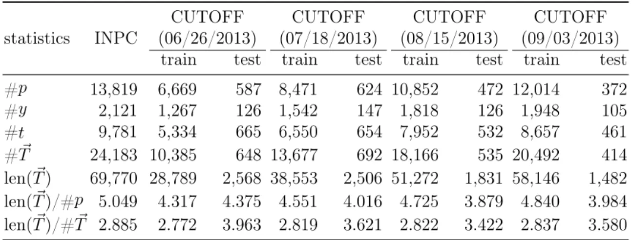
Table 3.3.: Statistics of INPC Dataset statistics INPC

CUTOFF CUTOFF CUTOFF CUTOFF

(06/26/2013) (07/18/2013) (08/15/2013) (09/03/2013) train test train test train test train test

#p 13,819 6,669 587 8,471 624 10,852 472 12,014 372 #y 2,121 1,267 126 1,542 147 1,818 126 1,948 105 #t 9,781 5,334 665 6,550 654 7,952 532 8,657 461 #T~ 24,183 10,385 648 13,677 692 18,166 535 20,492 414 len(T~) 69,770 28,789 2,568 38,553 2,506 51,272 1,831 58,146 1,482 len(T~)/#p 5.049 4.317 4.375 4.551 4.016 4.725 3.879 4.840 3.984 len(T~)/#T~ 2.885 2.772 3.963 2.819 3.621 2.822 3.422 2.837 3.580 In this table, #pis the number of patients; #y is the number of physicians; #tis the number of terms; #T~ is the number of sequences; len(T~) is total length of sequences; len(T~)/#pis average length of sequences per patient and len(T~)/#T~ is average length of sequences.

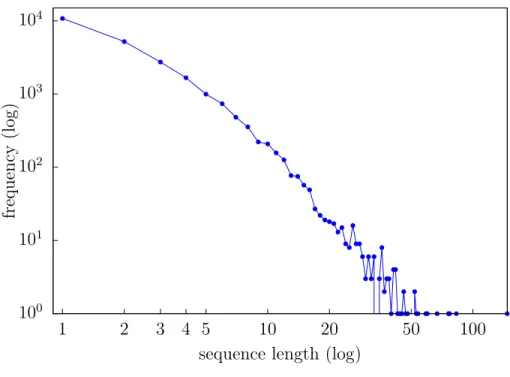
The data we use for experiments come from the Indiana Network for Patient Care (INPC)1. The INPC is Indiana’s major health information exchange, and offers physicians access to the most complete, cross-facility virtual electronic patient records in the nation. Implemented in the 1990s, the INPC collects data from over 140 Indiana hospitals, laboratories, long-term care facilities and imaging centers. We extracted the INPC search logs that were generated between 01/24/2013 to 09/24/2013. Table 3.8.1 presents the statistics of the INPC dataset. Figure 3.1 presents the distribution of sequence length in the dataset. It is notable that search sequences are typically very short (on average 2.89 search terms per each sequence). Figure 3.2 presents the distribution of the number of unique terms for each patient. On average, each patient has 3.85 unique search terms. The short sequences and small number of unique search terms per patient make the recommendation problem difficult, because the available data are very sparse.

1_{IRB Protocol # 1612682149 “Supporting information retrieval in the ED through collaborative} filtering”.

(35)

100 101 102 103 104 1 2 3 4 5 10 20 50 100 frequency ( log )

sequence length (log)

Fig. 3.1.: Distribution of INPC sequence length

100 101 102 103 1 2 3 4 5 10 20 50 100 frequency ( log )

# unique terms (log)

Fig. 3.2.: Distribution of INPC # unique terms per patient

3.8.2 Experimental Protocols and Evaluation Metric

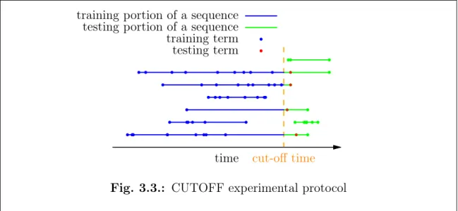
We use the following experimental protocol to evaluate our methods on the INPC dataset: all the search sequences are split by the same cut-off time. Any searches

(36)

cut-off time

time training portion of a sequence testing portion of a sequence training term testing term

Fig. 3.3.: CUTOFF experimental protocol

before the cut-off time are in the training set, and any searches after the cut-off time are in the test set. The models are trained using only training set, for example, the transition probabilities (Equation 3.4) are constructed only using the search se-quences and terms in training set, and the various similarities (Equation 3.11, 3.12 and 3.13) are calculated only from the training set. This protocol is referred to as cut-off cross validation, denoted as CUTOFF. Figure 3.3 demonstrates the CUTOFF experimental protocol. We use the cut-off time 08/15/2013. This cut-off time is selected because sufficient search terms from a majority of the search sequences are retained in training set before the cut-off time and meanwhile sufficient search se-quences have testing terms after the cut-off time. We also try other different cut-off times, including 06/26/2013, 07/18/2013 and 09/03/2013. After the split, the statis-tics for the training and test data are presented in Table 3.8.1 (in “CUTOFF” rows). This CUTOFF setting is close to the realistic scenario, that is, all the data before a certain time should be used to predict information after that time. However, a short-coming of CUTOFF is that many early search sequences may not have test terms, and many late search sequences will not have anything in the training set. Sequences that do not have test terms are still used to train models. Sequences that do not have

(37)

training terms are not used. For those sequences which have terms after the cut-off time, only the first one of the terms after the cut-off time will be used for evaluation. The model performance is measured using Hit-Rate at N (HR@N). For a se-quence, a hit is defined as a recommended term that is truly the next search term. HR@N is the percentage of testing sequences that have a hit and the hit appears among the top-N recommended terms. Higher HR@N values indicate better perfor-mance.

3.9 Experimental Results and Discussions

3.9.1 Overall Performance

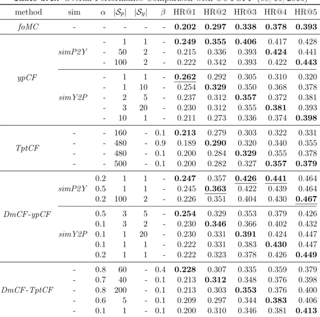
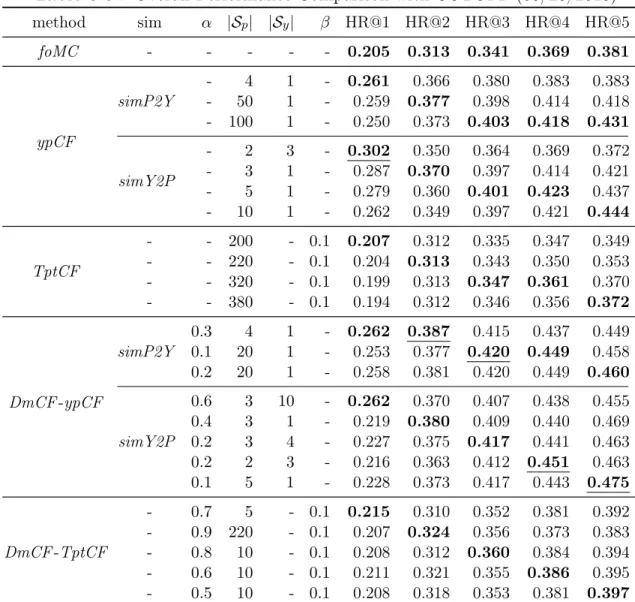
We compare foMC, ypCF, TptCF and DmCF, as well as their variations, in our experiments. Table 3.4 presents the best performance of each method. Overall, DmCF-ypCF with simP2Y is the best method because 4 out of 5 results of DmCF -ypCF with simP2Y are the best among all the methods. With parameters α=0.2, |Sp|=1 (i.e., 1 similar patient) and |Sy|=1 (i.e., 1 similar physician), DmCF-ypCF withsimP2Y outperforms the simplefoMC at 22.3%, 20.2%, 26.0%, 16.7% and 18.1% on HR@1, HR@2, HR@3, HR@4 and HR@5, respectively. The second best method is ypCF with simP2Y because it has better results overall than the rest methods. With parameters |Sp|=1 and |Sy|=1, ypCF with simP2Y outperforms the simple foMC at 23.3%, 19.5%, 20.1%, 10.3% and 8.9% on HR@1, HR@2, HR@3, HR@4 and HR@5, respectively. It is notable that although ypCF is significantly better than foMC, the bestDmCF-ypCF withsimP2Y has a weightα=0.2 on theypCF scoring component, but a weight 1-α=0.8 on the foMC scoring component. This indicates the importance of search dynamics in recommending the next search terms. It is also notable that the optimal DmCF-ypCF with simP2Y corresponds to a very small number of similar patients (Sp=1) and physicians (Sy=1). This demonstrates the effectiveness ofDmCF-ypCF in identifying most relevant information and leveraging such information for term recommendation.

(38)

Table 3.4.: Overall Performance Comparison with CUTOFF (08/15/2013) method sim α |Sp| |Sy| β HR@1 HR@2 HR@3 HR@4 HR@5 foMC - - - 0.202 0.297 0.338 0.378 0.393 ypCF simP2Y - 1 1 - 0.249 0.355 0.406 0.417 0.428 - 50 2 - 0.215 0.336 0.393 0.424 0.441 - 100 2 - 0.222 0.342 0.393 0.422 0.443 simY2P - 1 1 - 0.262 0.292 0.305 0.310 0.320 - 1 10 - 0.254 0.329 0.350 0.368 0.378 - 2 5 - 0.237 0.312 0.357 0.372 0.381 - 3 20 - 0.230 0.312 0.355 0.381 0.393 - 10 1 - 0.211 0.273 0.336 0.374 0.398 TptCF - - 160 - 0.1 0.213 0.279 0.303 0.322 0.331 - - 480 - 0.9 0.189 0.290 0.320 0.340 0.355 - - 480 - 0.1 0.200 0.284 0.329 0.355 0.378 - - 500 - 0.1 0.200 0.282 0.327 0.357 0.379 DmCF-ypCF simP2Y 0.2 1 1 - 0.247 0.357 0.426 0.441 0.464 0.5 1 1 - 0.245 0.363 0.422 0.439 0.464 0.2 100 2 - 0.226 0.351 0.404 0.430 0.467 simY2P 0.5 3 5 - 0.254 0.329 0.353 0.379 0.426 0.1 3 2 - 0.230 0.346 0.366 0.402 0.432 0.1 1 20 - 0.230 0.331 0.391 0.424 0.447 0.1 1 1 - 0.222 0.331 0.383 0.430 0.447 0.2 1 1 - 0.222 0.323 0.378 0.426 0.449 DmCF-TptCF - 0.8 60 - 0.4 0.228 0.307 0.335 0.359 0.379 - 0.7 40 - 0.1 0.213 0.312 0.348 0.376 0.398 - 0.8 200 - 0.1 0.213 0.303 0.353 0.376 0.400 - 0.6 5 - 0.1 0.209 0.297 0.344 0.383 0.406 - 0.1 1 - 0.1 0.200 0.310 0.346 0.381 0.413

In this table, the column “sim” corresponds to similarity identification methods;αis the weight on CF component inDmCF;|Sp|is the number of similar patients;|Sy|is the number of similar physicians;βis the similarity thresh-old to identify similar terms. The best performance of each method under each metric isbold. The best overall performance of all methods under each metric isunderlined.

The DmCF-TptCF method is also slightly better than foMC. With parameters α=0.1, |Sp|=1 and β=0.1, DmCF-TptCF outperforms foMC at -1.0%, 4.4%, 2.4%, 0.8% and 5.1% on HR@1, HR@2, HR@3, HR@4 and HR@5, respectively. However, DmCF-TptCF is significantly worse thanDmCF-ypCF withsimP2Y. The difference between DmCF-TptCF and DmCF-ypCF is that in DmCF-ypCF, the similarity-based scoring component (i.e., ypCF) does not consider search dynamics and only

(39)

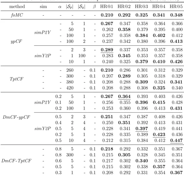
Table 3.5.: Overall Performance Comparison with CUTOFF (06/26/2013) method sim α |Sp| |Sy| β HR@1 HR@2 HR@3 HR@4 HR@5 foMC - - - 0.205 0.313 0.341 0.369 0.381 ypCF simP2Y - 4 1 - 0.261 0.366 0.380 0.383 0.383 - 50 1 - 0.259 0.377 0.398 0.414 0.418 - 100 1 - 0.250 0.373 0.403 0.418 0.431 simY2P - 2 3 - 0.302 0.350 0.364 0.369 0.372 - 3 1 - 0.287 0.370 0.397 0.414 0.421 - 5 1 - 0.279 0.360 0.401 0.423 0.437 - 10 1 - 0.262 0.349 0.397 0.421 0.444 TptCF - - 200 - 0.1 0.207 0.312 0.335 0.347 0.349 - - 220 - 0.1 0.204 0.313 0.343 0.350 0.353 - - 320 - 0.1 0.199 0.313 0.347 0.361 0.370 - - 380 - 0.1 0.194 0.312 0.346 0.356 0.372 DmCF-ypCF simP2Y 0.3 4 1 - 0.262 0.387 0.415 0.437 0.449 0.1 20 1 - 0.253 0.377 0.420 0.449 0.458 0.2 20 1 - 0.258 0.381 0.420 0.449 0.460 simY2P 0.6 3 10 - 0.262 0.370 0.407 0.438 0.455 0.4 3 1 - 0.219 0.380 0.409 0.440 0.469 0.2 3 4 - 0.227 0.375 0.417 0.441 0.463 0.2 2 3 - 0.216 0.363 0.412 0.451 0.463 0.1 5 1 - 0.228 0.373 0.417 0.443 0.475 DmCF-TptCF - 0.7 5 - 0.1 0.215 0.310 0.352 0.381 0.392 - 0.9 220 - 0.1 0.207 0.324 0.356 0.373 0.383 - 0.8 10 - 0.1 0.208 0.312 0.360 0.384 0.394 - 0.6 10 - 0.1 0.211 0.321 0.355 0.386 0.395 - 0.5 10 - 0.1 0.208 0.318 0.353 0.381 0.397

looks at the search terms that have ever been searched by similar physicians on similar patients, regardless of how such search terms transit to the search term of interest, whileTptCF considers such transitions. The performance difference betweenDmCF -TptCF and DmCF-ypCF may indicate that the transition information captured in TptCF might overlap with that captured infoMC and thus combining them together will not lead to substantial gains. On the other hand, the information captured by

(40)

Table 3.6.: Overall Performance Comparison with CUTOFF (07/18/2013) method sim α |Sp| |Sy| β HR@1 HR@2 HR@3 HR@4 HR@5 foMC - - - 0.210 0.292 0.325 0.341 0.348 ypCF simP2Y - 5 1 - 0.267 0.347 0.358 0.364 0.366 - 50 1 - 0.262 0.358 0.379 0.395 0.400 - 100 1 - 0.257 0.358 0.384 0.402 0.412 - 100 2 - 0.237 0.342 0.380 0.396 0.413 simY2P - 2 3 - 0.289 0.337 0.353 0.357 0.358 - 1 100 - 0.283 0.345 0.353 0.357 0.358 - 10 1 - 0.240 0.325 0.379 0.410 0.426 TptCF - - 260 - 0.1 0.210 0.286 0.301 0.312 0.329 - - 300 - 0.1 0.207 0.289 0.305 0.318 0.329 - - 380 - 0.1 0.208 0.288 0.309 0.324 0.341 - - 420 - 0.1 0.208 0.288 0.308 0.325 0.340 DmCF-ypCF simP2Y 0.2 5 1 - 0.267 0.364 0.393 0.403 0.426 0.1 50 1 - 0.256 0.355 0.396 0.415 0.428 0.2 100 1 - 0.253 0.360 0.396 0.413 0.431 simY2P 0.5 2 3 - 0.251 0.347 0.387 0.408 0.426 0.4 2 4 - 0.250 0.351 0.392 0.413 0.431 0.5 5 4 - 0.228 0.341 0.397 0.419 0.441 0.2 5 1 - 0.228 0.335 0.389 0.423 0.436 0.5 10 4 - 0.212 0.315 0.384 0.412 0.447 DmCF-TptCF - 0.8 5 - 0.1 0.218 0.292 0.332 0.351 0.367 - 0.8 300 - 0.1 0.215 0.305 0.328 0.345 0.351 - 0.6 5 - 0.1 0.217 0.302 0.340 0.355 0.364 - 0.5 5 - 0.1 0.215 0.302 0.338 0.357 0.364 - 0.3 1 - 0.1 0.208 0.292 0.331 0.354 0.367

ypCF methods could be complementary to that in foMC and thus integration of ypCF and foMC results in significant performance improvement.

In DmCF-ypCF, simP2Y is slightly better than simY2P. The simP2Y method first identifies patients similar to the target patient, and based on the identified simi-lar patients identifies physicians simisimi-lar to the target physician. ThesimY2P method identifies similar patients and similar physicians in the reversed order as in simP2Y.

(41)

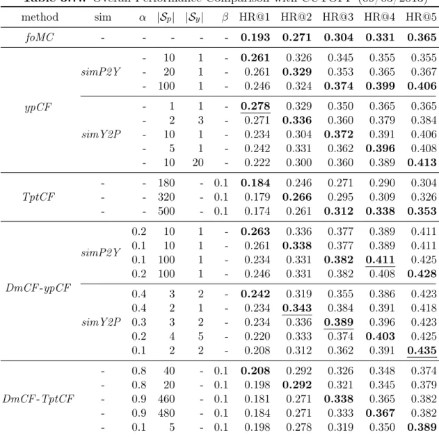
Table 3.7.: Overall Performance Comparison with CUTOFF (09/03/2013) method sim α |Sp| |Sy| β HR@1 HR@2 HR@3 HR@4 HR@5 foMC - - - 0.193 0.271 0.304 0.331 0.365 ypCF simP2Y - 10 1 - 0.261 0.326 0.345 0.355 0.355 - 20 1 - 0.261 0.329 0.353 0.365 0.367 - 100 1 - 0.246 0.324 0.374 0.399 0.406 simY2P - 1 1 - 0.278 0.329 0.350 0.365 0.365 - 2 3 - 0.271 0.336 0.360 0.379 0.384 - 10 1 - 0.234 0.304 0.372 0.391 0.406 - 5 1 - 0.242 0.331 0.362 0.396 0.408 - 10 20 - 0.222 0.300 0.360 0.389 0.413 TptCF - - 180 - 0.1 0.184 0.246 0.271 0.290 0.304 - - 320 - 0.1 0.179 0.266 0.295 0.309 0.326 - - 500 - 0.1 0.174 0.261 0.312 0.338 0.353 DmCF-ypCF simP2Y 0.2 10 1 - 0.263 0.336 0.377 0.389 0.411 0.1 10 1 - 0.261 0.338 0.377 0.389 0.411 0.1 100 1 - 0.234 0.331 0.382 0.411 0.425 0.2 100 1 - 0.246 0.331 0.382 0.408 0.428 simY2P 0.4 3 2 - 0.242 0.319 0.355 0.386 0.423 0.4 2 1 - 0.234 0.343 0.384 0.391 0.418 0.3 3 2 - 0.234 0.336 0.389 0.396 0.423 0.2 4 5 - 0.220 0.333 0.374 0.403 0.425 0.1 2 2 - 0.208 0.312 0.362 0.391 0.435 DmCF-TptCF - 0.8 40 - 0.1 0.208 0.292 0.326 0.348 0.374 - 0.8 20 - 0.1 0.198 0.292 0.321 0.345 0.379 - 0.9 460 - 0.1 0.181 0.271 0.338 0.365 0.382 - 0.9 480 - 0.1 0.184 0.271 0.333 0.367 0.382 - 0.1 5 - 0.1 0.198 0.278 0.319 0.350 0.389

The better performance ofsimP2Y oversimY2P inDmCF-ypCF demonstrates that when physician search dynamics has been considered viaMC, similar patients should be identified first and then based on identified similar patients, similar physicians should be identified. This may be because that when MC already considers all pa-tients and all physicians (Equation 3.4), a more focused and more homogeneous group of patients similar to the target patient is more critical in order to complement to the

(42)

MC information. Since physicians may see many patients with different diseases, high physician similarity may be due to patients who are different from the target patient. If such physicians are first selected (e.g., in simY2P), similar patients identified from these physicians might be very different from the target patient. However, when no information about all the patients and all the physicians is considered like in ypCF, a diverse set of physicians and patients might be beneficial, and that could explain why in ypCF, simY2P actually outperformssimP2Y slightly.

Table 3.5, Table 3.6 and Table 3.7 present the best performance of all the meth-ods for cut-off times 06/26/2013, 07/18/2013 and 09/03/2013, respectively. Overall, DmCF-ypCF achieves the best performance over the other methods on the different cut-off times. The trends among different methods as identified from cut-off time 08/15/2013 remain very similar for the other cut-off times. Note that as using later cut-off times, training data become more as shown in Table 3.8.1, and the performance of each method over different cut-off times tends to become worse. For example, the performance of foMC model decreases in general over different cut-off times. This may be due to the increasing heterogeneity among patients as more patients in the system. Table 3.5 presents the best performance of all the methods for cut-off time 06/26/2013. Overall,DmCF-ypCF withsimP2Y and simY2P are the best methods because 4 out of 5 results of DmCF-ypCF with simP2Y and simY2P are the best among all the methods. The best HR@1 is achieved with the parameters |Sp|=2 (i.e., 2 similar patients) and |Sy|=3 (i.e., 3 similar physicians) ofypCF withsimY2P method. The best HR@2, HR@3, HR@4 and HR@5 are achieved by theDmCF-ypCF with simP2Y and simY2P methods. The best HR@2, HR@3, HR@4 and HR@5 are better than the performance offoMC with the improvements of 23.6%, 23.2%, 22.2% and 24.7%. Table 3.6 presents the best performance of all the methods for cut-off time 07/18/2013. Overall, DmCF-ypCF with simP2Y and simY2P are the best methods because 4 out of 5 results of DmCF-ypCF with simP2Y and simY2P are the best among all the methods. The best HR@1 is achieved with the parameters |Sp|=2 (i.e., 2 similar patients) and |Sy|=3 (i.e., 3 similar physicians) of ypCF with

(43)

simY2P method. The best HR@2, HR@3, HR@4 and HR@5 are achieved by the DmCF-ypCF with simP2Y and simY2P methods. The best HR@2, HR@3, HR@4 and HR@5 are better than the performance offoMC with the improvements of 24.7%, 22.2%, 24.0% and 28.4%. Table 3.7 presents the best performance of all the meth-ods for cut-off time 09/03/2013. Overall, DmCF-ypCF with simP2Y and simY2P are the best methods because 4 out of 5 results of DmCF-ypCF with simP2Y and simY2P are the best among all the methods. The best HR@1 is achieved with the parameters |Sp|=1 (i.e., 1 similar patient) and |Sy|=1 (i.e., 1 similar physician) of ypCF withsimY2P method. The best HR@2, HR@3, HR@4 and HR@5 are achieved by the DmCF-ypCF with simP2Y and simY2P methods. The best HR@2, HR@3, HR@4 and HR@5 are better than the performance of foMC with the improvements of 26.6%, 28.0%, 24.2% and 19.2%. Overall, the best performance is achieved by the method DmCF-ypCF. The trends are also similar for different cut-off times.

Comparing ypCF and TptCF, it is notable that ypCF is significantly better than TptCF, even though in TptCF more patients similar to the target patient are used to achieve its optimal performance. In TptCF, only terms from similar physicians and patients that are similar to the term of interest are considered in calculating the scores (Equation 3.10). However, in ypCF, all the terms from similar physicians and patients are used. The improved performance of ypCF compared to that of TptCF may indicate that using more possible terms could benefit recommendation. On the other hand, bothfoMC andTptCF consider term transitions, whileTptCF considers term transitions only among similar terms on similar patients. The experimental results show thatTptCF performs worse thanfoMC. This may indicate that if term transition is a major factor in determining next search term, transitions from more diverse patients should be integrated.

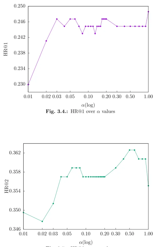
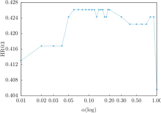
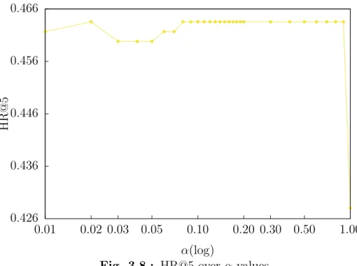
Figure 3.4, 3.5, 3.6, 3.7 and 3.8 present HR@1, HR@2, HR@3, HR@4 and HR@5 of DmCF-ypCF with simP2Y over different α values (Equation 3.2) when |Sy| = 1 and |Sp| = 1. As the weight α increases from 0, that is, as the CF takes place in the term scoring (Equation 3.2), the performance of DmCF in terms of HR@1,

(44)

0.230 0.234 0.238 0.242 0.246 0.250 0.01 0.02 0.03 0.05 0.10 0.20 0.30 0.50 1.00 HR@1 α(log)

Fig. 3.4.: HR@1 overα values

0.346 0.350 0.354 0.358 0.362 0.01 0.02 0.03 0.05 0.10 0.20 0.30 0.50 1.00 HR@2 α(log)

(45)

0.404 0.408 0.412 0.416 0.420 0.424 0.428 0.01 0.02 0.03 0.05 0.10 0.20 0.30 0.50 1.00 HR@3 α(log)

Fig. 3.6.: HR@3 overα values

0.416 0.420 0.424 0.428 0.432 0.436 0.440 0.444 0.01 0.02 0.03 0.05 0.10 0.20 0.30 0.50 1.00 HR@4 α(log)

(46)

0.426 0.436 0.446 0.456 0.466 0.01 0.02 0.03 0.05 0.10 0.20 0.30 0.50 1.00 HR@5 α(log)

(47)

HR@2 and HR@3 generally increases. For the performance of HR@4 and HR@5, as the weightα increases from 0, the performance slightly decreases, then increases and becomes stable (except when α=1 which means only the CF scoring component is considered.). This demonstrates the effect from CF scoring component in DmCF. As α further increases, the performance in general first gets better and then worse (except that the HR@1 performance reaches its best atα=1). This indicates that the dynamic scoring component and CF scoring component in DmCF play complemen-tary roles for recommending terms, and thus considering their combination enables better recommendation performance than each of the two methods alone.

3.9.2 Similarity Analysis 0.01% 0.1% 1% 10% 0.0 0.1 0.2 0.3 0.4 0.5 0.6 0.7 0.8 0.9 1.0 nnz % ( log ) simy

Fig. 3.9.: Physician-physician similarity distribution

Figure 3.9 and 3.10 present the distribution of non-zero physician-physician simi-larities (simy) and patient-patient simisimi-larities (simp), respectively. Figure 3.11 presents the distribution of non-zero term-term similarities (sim_t). For simy, 5.65% of

(48)

physician-0.001% 0.01% 0.1% 1% 10% 0.0 0.1 0.2 0.3 0.4 0.5 0.6 0.7 0.8 0.9 1.0 nnz % ( log ) simp

Fig. 3.10.: Patient-patient similarity distribution

0.01% 0.01% 0.1% 1% 10% 0.0 0.1 0.2 0.3 0.4 0.5 0.6 0.7 0.8 0.9 1.0 non-zero p erce n tage ( log ) sim_t

(49)

physician similarities are non-zero, and 80.98% of the non-zero similarities are less than or equal to 0.2. For simp, 2.65% of the patient-patient similarities are non-zero, and 77.05% of the non-zero similarities are less than or equal to 0.5. For sim_t, only 0.28% of term-term similarities are non-zero, and 78.36% of the non-zero similarities are less than or equal to 0.3. Specially, there are some patients whose similarities with one another are relatively high (i.e., the peaks in Figure 3.10 on larger simp values). This also explains the advantages of simP2Y oversimY2P and their performance in Table 3.4, because more patients with higher simpto the target patient provide better opportunities for DmCF to identify relevant information from such similar patients.

3.10 Conclusions

In this chapter, we presented our new dynamic and multi-collaborative filtering methodDmCF to recommend search terms relevant to patients for physicians. DmCF combines a dynamic first-order Markov chain model and a multi-collaborative filter-ing model in order to score and prioritize search terms. The collaborative filterfilter-ing model leverages the key idea originating from Recommender Systems research, and uses patient similarities, physician similarities and term similarities to score potential search terms. The linear combination of the dynamic-based scoring and the multi-collaborative filtering-based scoring is able to produce high quality recommendations that are most relevant to the patients and that are most interested to physicians.

(50)

4. LOCAL SPARSE LINEAR MODEL ENSEMBLE FOR

TOP-N

RECOMMENDATION

4.1 Introduction

Top-N Recommender Systems (RS) have been widely used in E-commerce appli-cations. However, two typical issues still challenge the current top-N RS development: 1). data sparsity, when there are not sufficient data to train a good RS model, and 2). user/item heterogeneity, when a global model (e.g., the popular matrix factorization models) trained from all the users/items fail for certain users/items. Existing meth-ods that tackle the first issue include factorized models [27] and implicit feedback based models [28], etc. Emerging methods dealing with the second issue include the most recent local model based approaches [29, 30].

In this paper, we develop local sparse linear model ensemble to tackle both the data sparsity and the user/item heterogeneity issues. We learn multiple local Sparse LInear Models (SLIM) [11] for all the users and items in the system. These models are then combined in various ways to produce top-N recommendations. SLIMis strong in learning relations among items, while localizing SLIMwith respective to certain users and items better reveal localized item relations among a certain group of users. By combining multiple SLIM models, signals from multiple models are aggregated so as to enable better results for sparse data. Our experiments over datasets of different sparsity levels demonstrate the superior performance of the model ensemble method.