A Random Forest Assisted Evolutionary Algorithm
for Data-Driven Constrained Multi-Objective
Combinatorial Optimization of Trauma Systems
Handing Wang,
Member, IEEE,
Yaochu Jin,
Fellow, IEEE
Abstract—Many real-world optimization problems can be solved by using the data-driven approach only, simply because no analytic objective functions are available for evaluating candidate solutions. In this work, we address a class of expensive data-driven constrained multi-objective combinatorial optimization problems, where the objectives and constraints can be calculated only on the basis of large amount of data. To solve this class of problems, we propose to use random forests and radial basis function networks as surrogates to approximate both objective and constraint functions. In addition, logistic regression models are introduced to rectify the surrogate-assisted fitness evaluations and a stochastic ranking selection is adopted to further reduce the influences of the approximated constraint functions. Three variants of the proposed algorithm are empirically evaluated on multi-objective knapsack benchmark problems and two real-world trauma system design problems. Experimental results demonstrate that the variant using random forest models as the surrogates are effective and efficient in solving data-driven constrained multi-objective combinatorial optimization problems.
Index Terms—Data-driven optimization, constrained multi-objective combinatorial optimization, evolutionary algorithm, surrogate, random forest, radial basis function networks, trauma systems
I. INTRODUCTION
Many real-world applications involve solving constrained combinatorial optimization problems whose feasible regions are not convex, seriously limiting the search capability of mathematical programming methods [1]. Therefore, meta-heuristics such as evolutionary algorithms (EAs) have recently become popular for handling combinatorial optimization [2], [3]. The use of EAs to solve combinatorial optimization be-comes less practical, however, when fitness evaluations of can-didate solutions rely on time-consuming numerical simulations or expensive physical experiments rather than computationally cheap analytic functions [4]. Optimization problems that are solved with the help of simulation, experimental or other types
This work was supported in part by an EPSRC grant (No. EP/M017869/1) and in part by the National Natural Science Foundation of China (No. 61590922). (Corresponding author: Yaochu Jin)
H. Wang is with School of Artificial Intelligence, Xidian University, Xi’an 710071, China. The work was done when she was with the Department of Computer Science, University of Surrey, Guildford, GU2 7XH, UK. (e-mail: [email protected]).
Y. Jin is with the Department of Computer Science, University of Surrey, Guildford, GU2 7XH, U.K. He is also affiliated with the Department of Computer Science and Technology, Taiyuan University of Science and Tech-nology, Taiyuan 030024, China, and the State Key Laboratory of Synthetical Automation for Process Industries, Northeastern University, Shenyang, China. (e-mail: [email protected]).
of data are termed data-driven optimization [5]. Typically, surrogates [4] need to be built using the data to substitute the fitness function, in part or completely, in data-driven optimization. According to [5], data-driven surrogate-assisted optimization can be divided into offline and online data-driven, depending on whether a certain amount of new data can be made available during the optimization process. In the last decade, data-driven surrogate-assisted evolutionary algorithms (SAEAs) [6] have found many successful real-world applica-tions, such as aerodynamic design [7], [8], microwave design [9], furnace design [10], and circuit design [11].
Most existing SAEAs have been developed for online data-driven optimization of continuous problems, where appropriate surrogates are chosen and model management strategies are designed to make sure that the EA is able to find the best solution with the given computation budget [12]. A wide range of regression models have been adopted as the surrogates, such as Kriging model (Gaussian processes regression model) [13], [14], radial basis function (RBF) networks [15]–[18], polynomial regression [19], and artificial neural networks [20], [21]. Since different regression models have different strengths and weaknesses, multiple surrogate models are combined as an ensemble in a single SAEA to increase its robustness [22]– [25].
Model management strategies distinguish themselves mainly in the criteria for selecting new candidate solutions to be evaluated using the expensive objective functions [4]. In generation-based model management strategies, the updating frequency can be fixed [21] or self-adaptive [20]. In individual-based model management strategies, promising and uncertain solutions according to the surrogate model [26]–[28] are eval-uated using the expensive objective functions. A large number of SAEAs for single-objective optimization [6], [25], [29], [30], multi-objective optimization [12], [22], [31], [32], and many-objective optimization [13], [33] have been proposed.
By contrast, very few SAEAs have been dedicated to expen-sive data-driven mixed-integer or combinatorial optimization problems [34]. Typically, regression models widely used for surrogate-assisted continuous optimization are directly adopted as surrogates for mixed-integer optimization problems [35]– [37] or combinatorial optimization [38]–[40]. Note that many combinatorial optimization problems can be better solved by incorporating domain knowledge, where surrogate models can be helpful [41]–[43].
Likewise, relatively little work has been carried out on surrogate-assisted optimization of constrained problems [44].
Constraints become relevant for SAEAs in different situations. For example, the evaluation of the constraint functions may be time-consuming, and consequently, surrogates need to be built for constraints [29], [45], [46]. Since constraints can be handled using penalty functions [47], surrogates are built to approximate the penalty function instead of the individual constraint functions [48], [49]. As whether a candidate solution is feasible or not can be seen as a classification problem, support vector machine [50], [51], k-nearest neighbors algo-rithm [52], and linear hyper-plane estimator [53] have been employed to distinguish feasible solutions from infeasible ones. Surrogates were also used as a way of manipulating the feasible regions to facilitate the EA to find the global optimum possibly located in an isolated region [54]. Even if the constraint functions are computationally inexpensive, they can still have considerable impact on SAEAs. For example, it has been found in [55] whether the infeasible samples should be used for training the surrogates have significant influences on the search performance of SAEAs.
To summarize, most existing data-driven surrogate-assisted optimization algorithms are developed for solving non-constrained continuous optimization problems despite the fact that many real-world problems are constrained combinatorial optimization problems. To fill the gap, this work aims to deal with a class of data-driven constrained multi-objective combinatorial optimization problems, where each evaluation of the objectives and constraints involves a large amount of historical data and therefore is time-consuming. Since EAs typically need a large number of fitness evaluations, the optimization process can become computationally intensive, even if one single evaluation is not particularly computa-tionally expensive. The main contributions of this work are summarized as follows.
• An in-depth investigation of random forest (RF) assisted evolutionary optimization of expensive multi-objective constrained combinatorial problems is performed. This includes the scalability of the performance to the dimen-sion of the search space, the influence of dimendimen-sion re-duction techniques and a comparison with the RBF-based surrogates. Note that research on RF-assisted evolutionary optimization has been reported for parameter tuning of a general algorithm [35] and surrogate-assisted genetic programming for symbolic regression [56], although the problems addressed therein are low-dimensional non-constrained single-objective problems.
• Logistic regression models are introduced to rectify the non-dominated ranking according to the surrogates for the constraint functions, as it is found that the EA is more likely to be misled by the approximated constraint functions than the approximated objective functions in the problems studied in this work. Additionally, stochastic ranking based on two selection criteria [57] is employed to further reduce the influence of the approximated con-straint functions.
• The performance of the proposed RF-assisted MOEA variants are studied in comparison with an RBF-assisted MOEA and three existing MOEAs without using
surro-gates on the multi-objective knapsack problems (MOKPs) up to 100 decision variables. In addition, the proposed algorithms are applied to two real-world trauma system design problems, one involving 18 hospitals with 40,000 data records collected in Scotland and the other involving 72 hospitals with 100,000 records collected in Colorado in the US. The results show that the RF-assisted MOEA is able to achieve satisfactory non-dominated solutions using a limited computation budget.
The remainder of the paper is organized as follows. In Section II, the main components of the proposed algorithm are described in detail. Empirical results on MOKPs are pre-sented and analyzed in Section III. Furthermore, we apply the proposed algorithm to two real-world trauma system design problems in Section IV. Section V concludes the paper.
II. PROPOSEDALGORITHM
A. Constrained Multi-Objective Combinatorial Optimization Problems
Generally, a combinatorial optimization problem with m
objectives and h inequality constraints can be described as follows:
minF(x) = (f1(x), ..., fm(x))T
s.t. G(x) = (g1(x), ..., gh(x))T ≤0
(1)
wherex is an n-dimensional decision variable vector whose domain is a set of finite elements. The m objectives are often conflicting with each other, thus there is no single ideal solution that can achieve the optimal value of all objectives. Like in continuous multi-objective optimization problems (MOPs), the optimal solution set is denoted as Pareto set (PS), whose corresponding objective values are called Pareto front (PF) [58]. Note that this work focuses on constrained multi-objective combinatorial optimization problems with two and three objectives.
B. General Framework
Over the past two decades, a large number of multi-objective optimization evolutionary algorithms (MOEAs) have been developed for solving MOPs with two or three objectives [59]. Generally, MOEAs can be divided into dominance based approaches, such as NSGA-II [60], decomposition based proaches, e.g., MOEA/D [61], and performance driven ap-proaches [62]. To solve data-driven constrained multi-objective combinatorial optimization problems, this paper proposes an SAEA using the dominance based approach [60]. Since the objectives and constraints can be evaluated using historical data only, surrogates (Fˆ(x)for objective functions andGˆ(x) for constraints) are constructed. For convenience, we call the algorithm using RF models [63] random forest assisted constrained multi-objective combinatorial optimization (RF-CMOCO), and the algorithm using RF models after feature selection RF-CMOCO(FS). Since the RBF model is one of few surrogate models that have been adopted for data-driven combinatorial optimization problems [36], [37], we replace the RF model in RF-CMOCO with the RBF model, which is the third variant studied in this work called RBF-CMOCO.
Initialization Stop? Generate offspring by crossover and mutation Stochastic ranking Select parent population Training dataset Randomly sample a
number of solutions and evaluate them by
exact function evaluations
Surrogate models for m objectives Surrogate models
for h constraints
Select solutions from the population and evaluate them by
exact function evaluations
Add those samples to training dataset
Output the non-dominated solutions of training dataset
Evaluate both parent and offspring populations:
Predict the objective and constraint values by surrogate models
Constraint correction Y N Feature selection Feature selection Start End
Fig. 1. A diagram of the proposed framework.
A diagram of the proposed framework is shown in Fig. 1. It consists of two main parts, an evolutionary optimizer and a model management strategy. Surrogate models form objec-tives and hconstraints are built separately on the basis of the training dataset, where a feature selection (FS) technique can be employed to reduce the dimension of decision space. The evolutionary optimizer searches for feasible optimal solutions based on the cheap surrogate models. An individual-based model management strategy [26] is adopted, where a number of promising solutions from the current population are selected and evaluated using the expensive objective and constraint functions. In SAEAs, solutions whose predicted fitness is better than the best solution found so far, or whose predicted fitness has a large degree of uncertainty are considered to be promising. These new data are then added to the training dataset for updating the surrogates. The proposed framework begins with a number of randomly sampled solutions (which are the initial training dataset for the surrogates) and finally outputs a set of non-dominated solutions. To reduce the impact resulting from the errors introduced by the approximated constraints, a logistic regression model is trained for each constraint to rectify the boundaries distinguishing feasible solutions from infeasible ones. Finally, the population is sorted based on stochastic ranking using two selection criteria, one based on the ranking as a constrained MOP, and the other on ranking as an unconstrained MOP.
C. Surrogate Modeling
1) Random Forest: Most surrogate models were designed for approximating continuous functions. Since the decision variables of combinatorial optimization problems are discrete, we use RF and RBF models as the surrogates to approximate themobjectives andhfunctions. Compared with RBF models, RF models have not been widely used as surrogates, although it has recently been suggested that the tree structure in RF models is well suited for approximating functions with discrete decision variables [34].
An RF model [63] is an ensemble of a large number of classification and regression trees (CARTs) [64], as illustrated
in Fig. 2. Each CART is trained by different bootstrap samples, which is the reason why thesektrees have different structures in Fig. 2. Given N training samples for an objective or a constraint function, d =(2b√nc) decision variables are randomly selected from the ntotal decision variables for the
N bootstrap samples of each tree [65]. Thus, one variable may be repeatedly included in a tree. The final output of the input x is the average of the outputs ofk trees. k is set to 100 in RF-CMOCO and RF-CMOCO(FS) as recommended in [66].
Fig. 2. An illustration of the random forest.
CART [64] has a binary tree structure, which is suited for the modeling discrete problems. CART divides the decision space into rectangle regions with leaf nodes, and the output of each leaf node is the average output of the samples in each divided region. Growing a CART is usually based on splitting and stopping criteria [67]. In CMOCO and RF-CMOCO(FS), the CART splits based on the minimization of the mean squared error (MSE) of the tree. It stops splitting when the reduction of the MSE is smaller than a pre-specified threshold, which is set to 1e−4∗σ2 (σ2 is the variance for
the entire data before the CART is grown) in the empirical studies.
m+hRF models formobjective andhconstraint functions are built separately. For each RF models,kCARTs are trained
using ksets of bootstrap samples. Thus,k×(m+h)CARTs are built for surrogate modeling in CMOCO and RF-CMOCO(FS).
2) Feature Selection: The amount of required data for training an RF model dramatically increases as the number of the decision variables increases. Therefore, we employ a feature selection technique for problems with more than 50 decision variables to reduce the input dimension before training the RF models for all m objective and h constraint functions. To this end, we employ the Kendall rank correlation coefficient (KRCC) [37] to measure the correlation between the decision variables and the objective or the constraint. Taking thei-th decision variablexias an example,N samples of xi and an objective in the training dataset are written as {(x1i, y1), ...,(xiN, yN)}. Any two samples (xji, yj) and (xk i, yk)are compared. Ifx j i > xki andyj> yk, or ifx j i < xki andyj< yk, the pair of samples is said to be concordant [68]. Ifxji > xki andyj< yk, or ifxji < xki andyj> yk, the pair of samples is said to be discordant [68]. The KRCC (τi) between
xi and the objective can be calculated as follows:
τ= nc−nd
N(N−1)/2 (2)
where nc is the number of concordant pairs and nd is the number of discordant pairs.τiranges within[−1,1], the closer
τi approximates to -1 or 1, the strongerxiis correlated to the objective. If τi = 0, xi and the objective are independent, namely, xi can be ignored when training the RF model for this particular objective or constraint.
Before training an RF model for approximating an objective or a constraint function, the KRCC between each decision variable and the objective or the constraint is calculated based on the training dataset. The contribution ratio of xi to the objective or the constraint is defined as:
Ri=
|τi|
Pn
j=1|τj|
(3)
which is the ratio of |τi|to the sum of all the absolute KRCC values. The contribution ratios of all the decision variables are sorted in a descending order. The selection of decision variables is based on the sorted order, i.e., the decision variable with a larger contribution ratio will have a higher priority to be selected. In the proposed algorithm, q decision variables are successively selected according to the sorting order until the accumulative contribution ratio of the selected decision variable amounts to 95%. Thus, q decision variables that are highly correlated with the objective or the constraint are retained. It is worth noting that q is not a parameter to be predefined by the user, rather it is problem-dependant. After selecting q decision variables, the setting for training the RF model changes accordingly. Thus, growing each CART is based on 2√qrandomly selected decision variables.
3) Model Management: In SAEAs, the model management strategy is responsible for selecting individuals to be eval-uated using the expensive objective functions and updating the surrogates. Most existing model management strategies have been developed for surrogate-assisted non-constrained optimization problems, which typically select solutions that
can help accelerate convergence and/or promote diversity to strike a balance between exploitation and exploration.
In this work, an individual-based model management strat-egy is proposed to deal with constrained optimization, aiming to take into account both convergence and constraint han-dling. Like other model management strategies, a number of solutions will be randomly generated and evaluated us-ing the expensive objective and constraint functions before optimization starts. All the randomly sampled solutions, no matter whether they are feasible or infeasible, are included in the initial training dataset for training the surrogates. Note, however, that the Latin hypercube sampling widely used for continuous optimization is not applicable for combinatorial optimization problems.
During the optimization, all offspring individuals at each generation will be evaluated at first using the surrogates. Then the individuals are sorted using the non-dominated sort [60], [69] according to degree of violation on the constraint func-tions (max{G(x),0}). Based on this order, solutions are suc-cessively determined whether they are potentially better than the non-dominated solutions in the training dataset (denoted by Pnd), which are the best-so-far solutions. Recall that all objective values of the solutions in the current generation are estimated using the surrogates. To account for the ap-proximation errors when comparing the solutions with those in Pnd, we calculate the root mean square errors (RMSEs) of m RF models for the objectives, which are denoted as End = {e1, ..., em}. Then, we use these errors to estimate the upper bound of the objective values of the solutions in the current generation. Let the estimated objective values of solution x be Fˆ(x), then the upper bound (best possible) objective values in case of minimization are assumed to be
ˆ
F(x)−End. If no solution inPndis able to dominate solution x according to its estimated best objective values, solution x will then be selected for evaluation using the expensive real fitness functions. The model management strategy is also outlined in Algorithm 1.
f1
f2 Non-dominated solutions of
training data
Predicted objective values of the population Estimated errors B C D A E F
Fig. 3. An illustration of the model management strategy for a 2-objective problem, wheref1 andf2 are two objectives.
Fig. 3 provides an illustrative example of a 2-objective problem, where the circles denote the non-dominated solu-tions in the training data (Pnd) and the dots (A-F) denote the individuals in the current population evaluated using the surrogates. Due to the approximation errors of the RF models, the true objective values of these solutions are indicated by the shaded rectangle and the best possible values are
Algorithm 1 Pseudo code for solution selection in model management.
Input: P: the population with the predicted objective and con-straint values (Fˆ(x)andGˆ(x)),Pnd: the non-dominated set of the training dataset, andNs: the number of solutions to be selected.
1: SetPsempty.
2: EstimatedEnd ofm RF models based onPnd.
3: P is sorted by the non-dominated sort on the predicted constraintsGˆ(x).
4: fori=1:|P|do
5: ifFˆ(xPi)−End is not dominatedPnd then 6: ifPi are not in the training dataset then
7: AddPi toPs. 8: end if 9: if|Ps| ≥Ns then 10: break 11: end if 12: end if 13: end for
14: Calculate the exact objective and constraint values ofPs.
Output: Ps
located at the bottom-left corner of the rectangle. Assume we intend to select two solutions from solutions A to F to be evaluated using the expensive objective functions. At first, the management strategy performs a non-dominated sort of the six solutions based on their predicted constraints Gˆ(x). Assume the resulting order is A, B, C, D, E and F, starting from the best. Now the sorted solutions are checked one by one to see whether they will be selected. Although solution A ranks the first, it is not able to dominate any solutions in
Pnd and consequently, solution A will not be selected. Then solution B is checked, which is found to be able to dominate one solution inPndby taking the estimation error into account (otherwise B will not be selected either). Solution C will also be selected as it is able to dominate one solution inPnd. Thus at this generation, solutions B and C are selected. Note that solution F is not selected since two solutions have already been chosen, even if it is the best solution according to the estimated objective values.
The proposed model management strategy hypothesizes that if the best solutions are far away from the infeasible region, convergence should be prioritized and therefore the better solutions should be selected. However, if the number of feasible solutions is very small, indicating the population is close to the infeasible region, constraint handling should be more important. In this case, infeasible solutions closest to the boundaries should be selected. Finally, the approximation errors are estimated by evaluating the surrogates using the non-dominated solutions in the training data so that potentially better solutions are selected and evaluated using the expensive objective and constraint functions.
D. Constraint Handling
In this work, constraints are approximated using surrogate models. Due to the approximation errors, some infeasible
solutions may be treated to be feasible, which will seriously mislead the evolutionary search. To mitigate this problem, we propose two novel constraint handling strategies in this section. 1) Logistic Regression for Constraint Correction: To re-duce the possibility of classifying feasible solutions to be infeasible, the first strategy we propose aims to rectify the boundaries between the feasible and infeasible regions defined by the surrogate constrained functions.
Take the situation illustrated in Fig. 4 as an example. In the figure, the solutions denoted by the plus signs are feasible ones and those by the cross signs are infeasible. Thej-th constraint
gj(x)is approximated by the surrogate modelgˆj(x). Because of approximation errors, two feasible solutions are classified as infeasible. If the constraint ˆgj(x)≤0 is changed togˆj(x)≤
αj, whereαj is the boundary between feasible and infeasible solutions, the misclassified solutions can be corrected.
ˆj g ˆ ( j) P g 0 Feasible solutions Infeasible solutions j
Fig. 4. An illustration of using logistic regression for constraint correction.
To rectify the boundary, we use a logistic regression model [70] to estimate the probability at which solution x with the approximated constraint value ˆgj(x)is feasible. The logistic regression model can be described as follows:
P(ˆgj) = 1
1 +eβ0+β1ˆgj (4)
where β0 and β1 are two parameters to be estimated. The training dataset is used to estimate the logistic regression model, where the predicted value ˆgj(x) of each sample is the input, and the probability of the solution being feasible is the output (gˆj(x) ≤ 0 is set to 1 and gˆj(x) > 0 is set to 0). Solutions are believed to be feasible for constraint gˆj when P(ˆgj) ≥0.95. Thus, the new boundary αj is defined as P(αj)=0.95, the constraint gj(x) ≤ 0 is changed to ˆ
gj(x)≤αj.
In each generation, after h surrogate models gˆj(x) (1 ≤
j ≤ h) are built, their feasible probabilities are learned by
h logistic regression models described in Eq. (4), then the boundariesαj are calculated. For the following selection, the problem is changed to Eq. (5) withαjoffset on the constraints.
min ˆF(x) = ( ˆf1(x), ...,fˆm(x))T
s.t.Gˆ(x) = (ˆg1(x)−α1, ...,gˆh(x)−αh)T ≤0 (5)
2) Stochastic Ranking Using Two Selection Criteria: It has been shown that the performance of handling constraints in SAEAs can be improved by converting constrained MOPs into unconstrained MOPs [71], [72], namely, constraints in Eq. (1) can be seen as additional objectives [44] as follows:
Thus, two selection criteria are available for sorting the population: ranking as an unconstrained MOP having m+h
objectives, or as a constrained MOP havingmobjectives and
hinequality constraints. A variety of efficient non-dominated sorting techniques can be used [69], [73].
Stochastic ranking [57] is a bubble-sort-like procedure, which was proposed to strike a balance between searching for better objectives and finding feasible solutions. In the original version of stochastic ranking, swapping adjacent solutions is based either on the objective values or on the constraint values at a certain probability. However, we adopt stochastic ranking in the proposed algorithm to balance two selection criteria, thereby further reducing the influence the approximation errors introduced by the approximated constraints.
Algorithm 2 Pseudo code for stochastic ranking using two selection criteria.
Input: P: population with the approximated objective and constraint values after constraint relaxation, NP: popu-lation size.
1: Ranking P as a unconstrained MOP by non-dominated sort, denoting asRU.
2: RankingP as a constrained MOP by non-dominated sort, denoting asRC. 3: fori=1:NP do 4: forj=1:|P| −1 do 5: ifU(0,1)<0.5then 6: ifRU j > RUj+1 then 7: SwapPj andPj+1.
8: SwapRUj andRUj+1, swapRCj andRCj+1.
9: end if
10: else
11: ifRjC> RCj+1 then
12: SwapPj andPj+1.
13: SwapRU
j andRUj+1, swapRCj andRCj+1. 14: end if
15: end if 16: end for
17: end for
Output: P with the firstNP solutions.
The stochastic ranking process in the proposed algorithm are described in Algorithm 2, whereU(0,1)is a random number in [0,1]. At each generation, a combination of the parent and offspring populationsP is evaluated using the surrogate mod-els, where the constraint boundaries have already been rectified using the logistic regression models. Before performing the stochastic ranking,P is ranked as an unconstrained MOP with
m+hobjectives and a constrained MOP withmobjectives and
h inequality constraints, respectively, the assigned ranks are denoted as RU and RC. In the bubble-sort, the comparisons between two adjacent solutions are based either onRU or on
RC at a probability of 0.5. Once the stochastic bubble-sort terminates, the first NP solutions in P are selected as the parents of the next generation.
E. Detailed Settings
The proposed framework involves surrogate modeling, op-timization, and constraint handling. For clarify, we summarize the parameter settings for the three variants of the proposed algorithm, RF-CMOCO, RF-CMOCO(FS), and RBF-CMOCO in Table I.
TABLE I
PARAMETER SETTINGS FORRF-CMOCO, RF-CMOCO(FS),AND
RBF-CMOCO
Component Parameter/ Settings Techique
Surrogate
Initial dataset
1000 random solutions
RF 100 CARTs that generated from the boot-strap samples of2√
n
randomly selected decision variables
CART Splitting tolerance is set to1e−4∗σ2(σ2
is the variance for the entire data) RBF n hidden nodes using the overlap
mea-sure [74] as the kernel function
FS Topqdecision variables with accumulative KRCC contribution ratio of 95%
Ns 5 exact function evaluations in each
gener-ation
Optimization PopulationBudget 100 solutions1500 or 2000 exact function evaluations Constraint
handling
Probability of feasibility
0.95
III. EXPERIMENTALSTUDIES
Unlike MOPs with continuous decision variables, multi-objective combinatorial optimization problems may have dif-ferent structures (or presentation) of decision variables [75]. For example, MOKPs have categorical decision variables, while multi-objective flow shop scheduling problems have per-mutation decision variables. For some structures like permu-tation decision variables, surrogate models cannot be directly used, and mapping- or similarity-based methods need to be applied [34]. Since the use of indirect surrogate models is out of the scope of this work, we choose MOKPs as the test problem, which can be generated by using the method reported in [76]. An MOKP with m objectives and n items can be modeled as follows: maxfi= n P j=1 vijxj, xj ∈ {0,1},1≤i≤m s.t. n P j=1 wjxj ≤W (7)
wherem objectives are the total values of the chosen items,
wj andvji are the weights and value for fi of the j-th item, and W is the weight limitation of the knapsack. Similar to the generation method in [76],wj andvji are random integers within [1,1000], and W is set to 0.5
n P j=1
wj. Based on the above method, we generate MOKP instances with 10 to 100 items and 2 to 3 objectives1. Here we assume each evaluation
in Eq. (7) is expensive. In this section, a fixed number of those expensive evaluations are set as the allowed computational budget of the compared algorithms.
A. Approximation Performance of Random Forest Models We first investigate the approximation performance of RF models for MOKPs. As the number of decision variables may heavily affect the performance of surrogates, we choose the first objectives of the 20-item MOKP as a low-dimensional test case and the 100-item MOKP as a high-dimensional test case. The experiment is conducted on the RF models with and without the feature selection for 30 independent times, where 100 to 2500 random solutions serve as the training dataset and 10,000 random solutions as the test dataset. In the experiment, we use the same settings for the RF models as recommended in [65], [66], which are presented in Table I.
The average RMSEs of the two RF models on the test dataset over the size of the training data are plotted in Fig. 5. From the figure, we can see that the performance of both RF models on 20- and 100-item MOKP instances enhances as the number of the training data increases. In the beginning, RMSEs of the two RF models drop rapidly when new data are added to the training dataset. However, the decrease of RMSEs becomes slow as the size of the training dataset further increases. In addition, it is noticed that feature selection can significantly enhance the performance of the RF model on the 100-item MOKP instance, but worsens the performance on the 20-item MOKP instance. These results indicate that feature selection significantly improves the performance of RF models in approximating functions with a large number of discrete variables. 0 500 1000 1500 2000 2500 400 500 600 700
Size of training dataset
R M SE n=20 RF RF with FS 0 500 1000 1500 2000 2500 1400 1600 1800 2000
Size of training dataset
R M SE n=100 RF RF with FS
Fig. 5. Average RMSEs of the RF models over the size of the training data with and without feature selection on two-objective MOKP instances with 20 and 100 items.
B. Constraint Handling Strategies
As shown in Fig. 5, the RMSE of the RF model re-mains very large even though the size of the training dataset has been increased to 2500, making it hard to distinguish feasible solutions from infeasible ones using the surrogate models. Therefore, additional constraint handling strategies are designed in this work. In this subsection, we evaluate the effectiveness of the proposed constraint handling strategies by performing experiments on a bi-objective MOKP instance with 20 items so that the influence of the objectives is minimized. As the experiments are conducted on the 20-item MOKP instance, no feature selection is applied in building the RF models.
The first strategy is to use logistic regression models to rectify the constraint boundaries. To examine the effectiveness of this strategy, we compare the performance of the RF models with and without the constraint correction strategy using the
0 20 40 60 80 100 180 200 220 240 260 280 Generation R M SE o f ap p ro xi m at ed c o n st ra in t RF model
RF model with constraint correction
0 20 40 60 80 100 160 180 200 220 240 Generation R M SE o f ap p ro xi m at ed c o n st ra in t RF model
RF model with constraint correction RF model trained by 1500 random samples RF model trained by 1000 random samples
Fig. 6. Average RMSEs of the RF models with and without constraint correction on the data generated by NSGA-II optimizing the bi-objective MOKP instance with 20 items.
data generated by NSGA-II of a population size 100. The experimental details are described in the following.
• Test datasets generation: Run the NSGA-II using ex-act function evaluations on the MOKP instance for 30 independent times, where the population size is set to 100 and a maximum of 100 generations are run. The 100 solutions generated in each generation are recorded as a dataset for evaluating the constraint handling strategies. Thus, 100 datasets are stored in each run.
• Constraint correction: For the 100 datasets generated in each run, two RF models are built from 1000 and 1500 random samples separately, then the boundaries separating the feasible and infeasible solutions α based on the two different strategies are calculated. Recall that the proposed constraint correction strategy changes their prediction of constraints toGˆ(x)−α.
• Performance evaluation: Predict the constraint values in every generation by the RF models with and without constraint correction. The RMSEs of the RF models are calculated for the solutions generated in each of the 100 generations.
The average RMSEs of the RF models with and without constraint correction in different generations are shown in Fig. 6. As the search proceeds, the population (the test dataset) becomes concentrated, the RMSE in local areas gradually increases. It can be observed that RF models trained using 1500 samples have a smaller RMSE than those trained using 1000 samples. It can also be seen that the constraint correction strategy reduces the RMSEs of both RF models. These results indicate that the logistic regression based correction strategy is able to improve the performance of the RF models of the constraint functions.
The second strategy we employ is a stochastic ranking strategy using two selection criteria to further reduce the influence of the approximation errors induced by the RF
models. We conduct the following experiments to demonstrate the effects of the stochastic ranking strategy.
• Generation of the test datasets: Run the NSGA-II using exact function evaluations on the MOKP instance for 30 independent times, where the population size and the terminal criterion are set as in the previous experiments. The combination of parent and offspring populations and the selected population Ps in each generation are recorded as the datasets for evaluating the stochastic ranking strategy.
• Prediction via surrogate models: For the 100 datasets generated in each run, two RF models are built using 1000 and 1500 random samples separately. Then the constraint correction strategy is applied on both models. Predict the objective and constraint values of the combined population in each generation using the RF models with the constraint correction strategy.
• Selection: For each generation, select populations (PsU,
PsC, andPsSR) from the combined population using three different ranking strategies, namely, ranking by consider-ing the MOKP as an unconstrained MOP, a constrained MOP, or the proposed stochastic ranking.
• Performance evaluation: Calculate the percentages of
PU
s ∩Ps,PsC∩Ps, andPsSR∩PsinPsas the selection accuracy. 0 20 40 60 80 100 0.4 0.6 0.8 1 Generation A cc u ra cy o f Se le ct io n 0 20 40 60 80 100 0.4 0.6 0.8 1 Generation A cc u ra cy o f Se le ct io n
RF model trained by 1500 random samples RF model trained by 1000 random samples
Ranking as an unconstrained MOP Ranking as a constrained MOP Stochastic Ranking
Fig. 7. Average selection accuracy of the three different ranking strategies based on the RF models trained using 1000 and 1500 random samples on a bi-objective MOKP instance with 20 items.
For the MOKP instance, the average selection performance of the three different ranking methods based on the RF models trained using 1000 and 1500 random samples in different generations are shown in Fig. 7. It can be seen that for both RF models, the selection accuracy of the ranking method considering the problem as a constrained MOP is about half of that of the ranking method considering the problem as an unconstrained MOP. However, stochastic ranking, which is a hybrid of these two ranking methods, is able to improve the
selection accuracy to 0.7. In particular in the early generations, the stochastic ranking can achieve much higher selection accuracy than the other two ranking strategies. As the search proceeds, however, the percentage of feasible solutions in the population gradually increases, the performance of the ranking strategy considering the problem as an unconstrained MOP rapidly improves and even becomes slightly better at the later generations. Nevertheless, the stochastic ranking maintains an overall satisfactory selection accuracy in the entire search process of NSGA-II. We also find that the selection based on the RF model trained using 1500 data samples performs slightly better, due to better-trained models.
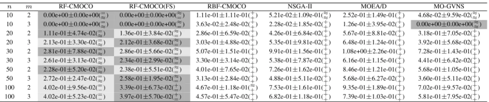
C. Comparative Experiments
In this section, RF-CMOCO, RF-CMOCO(FS), and RBF-CMOCO are compared with other algorithms on two- or three-objective MOKP instances with 10 to 100 items. Both mathematical programming and MOEAs have been employed for solving MOKPs [3]. The algorithms using mathemati-cal programming [77] require analytic functions of MOKPs, which does not meet the assumption that analytic objective and constraint functions are not available made in this work. Therefore, we choose two MOEAs for comparison.
• Generic MOEAs: NSGA-II [60] and MOEA/D [61] are two popular MOEAs without using any domain knowl-edge or local search strategy.
• Specific MOEAs: Variable neighborhood search (VNS) has been shown effective in solving MOKPs in [78], although analytic functions are used. For fair comparison, we include MO-GVNS [79], an MOEA with general VNS without using analytic functions, for comparison. In the experiments, a maximum of 1500 exact fitness evaluations is allowed, of which 1000 fitness evaluations are used for building the RF models before the optimization starts and 500 exact fitness evaluations can be used during the op-timization. All compared algorithms perform 30 independent times and they terminate when the allowed computation budget is exhausted. All algorithms under comparison use 3-point crossover with a probability of 1 and point mutations with a probability of 0.2. In the experiments, the settings of RF-CMOCOs and RBF-CMOCO are presented in Table I. The population size of MO-GVNS and NSGA-II is set to 100. The population size of MOEA/D (with the neighborhood parameter
T = 30 ) is set to 100 for 2-objective MOKPs and 105 for 3-objective MOKPs.
To evaluate the results obtained by the compared algorithms, inverted generational distance (IGD) [80], the average distance from a reference set to the obtained solution set, is adopted, which is believed to be able to account for both convergence and diversity. We use the non-dominated set of solutions obtained from 30 runs of NSGA-II (with a population size of 100 run for 200 generations using exact function evaluations) as the reference set for calculating IGD. Further, we normalize the objectives using the extreme points in the reference set. The IGD values of the compared algorithms on the MOKP instances are presented in Table II, where the comparisons between RF-CMOCOs (with and without feature selection)
TABLE II
THEIGDVALUES OFRF-CMOCOS(WITH AND WITHOUT FEATURE SELECTION), RBF-CMOCO, NSGA-II, MOEA/D,ANDMO-GVNSON THEMOKP
INSTANCES WITHnITEMSmOBJECTIVES. THE BEST AND SECOND BEST FITNESS VALUES AMONG ALL THE COMPARED ALGORITHMS FOR EACH
INSTANCE ARE HIGHLIGHTED IN GRAY AND LIGHT GRAY. THE RESULTS OFRF-CMOCOVARIANTS AND OTHER COMPARED ALGORITHMS ARE ANALYZED
USING THEWILCOXON SIGNED-RANK TEST(SIGNIFICANCE LEVEL=0.05). THE ANALYSIS RESULTS OFRF-CMOCOIS DENOTED AS THE SUPERSCRIPT IN
BRACKETS,WHILE THOSE OFRF-CMOCO(FS)ARE DENOTED AS THE SUBSCRIPT IN BRACKETS.
n m RF-CMOCO RF-CMOCO(FS) RBF-CMOCO NSGA-II MOEA/D MO-GVNS
10 2 0.00e+00±0.00e+00(=≈) 0.00e+00±0.00e+00(≈=) 1.11e-01±1.11e-01( +
+) 5.21e-02±1.09e-01( ≈
≈) 2.52e-01±1.49e-01(++) 4.68e-02±9.59e-02( ≈ ≈) 10 3 0.00e+00±0.00e+00(= ≈) 0.00e+00±0.00e+00( ≈ =) 3.63e-02±2.48e-02( + +) 2.28e-02±1.85e-02( + +) 1.26e-01±3.95e-02( + +) 0.00e+00±0.00e+00( ≈ ≈) 20 2 1.11e-01±4.74e-02(=≈) 1.36e-01±3.84e-02(≈=) 2.86e-01±6.59e-02(
+ +) 4.26e-01±6.84e-02( + +) 5.67e-01±8.81e-02( + +) 3.18e-01±7.05e-02( + +) 20 3 2.13e-01±3.30e-02(= ≈) 2.12e-01±3.68e-02( ≈ =) 3.03e-01±4.88e-02( + +) 5.35e-01±9.81e-02( + +) 6.48e-01±1.24e-01( + +) 3.92e-01±5.68e-02( + +)
30 2 2.81e-01±7.88e-02(=≈) 2.86e-01±5.66e-02(≈=) 5.07e-01±1.51e-01( + +) 9.91e-01±1.56e-01( + +) 1.08e+00±2.26e-01( + +) 7.28e-01±1.43e-01( + +) 30 3 2.61e-01±3.13e-02(= ≈) 2.34e-01±2.99e-02( ≈ =) 3.30e-01±3.14e-02( + +) 5.38e-01±7.87e-02( + +) 6.16e-01±1.15e-01( + +) 4.41e-01±6.42e-02( + +)
50 2 2.28e-01±5.20e-02(=≈) 2.38e-01±5.51e-02(≈=) 4.01e-01±7.65e-02( + +) 7.26e-01±1.62e-01( + +) 8.46e-01±1.21e-01( + +) 5.68e-01±1.05e-01( + +) 50 3 2.72e-01±2.47e-02(= ≈) 2.58e-01±1.95e-02( ≈ =) 3.13e-01±2.84e-02( + +) 4.88e-01±5.11e-02( + +) 5.68e-01±6.27e-02( + +) 3.60e-01±5.11e-02( + +)
100 2 4.02e-01±9.56e-02(=−) 3.39e-01±6.73e-02(+=) 4.67e-01±1.18e-01( ≈ +) 7.53e-01±1.61e-01( + +) 9.35e-01±1.89e-01( + +) 7.02e-01±9.57e-02( + +) 100 3 4.02e-01±5.23e-02(=
−) 3.97e-01±5.70e-02(+=) 4.57e-01±5.47e-02( + +) 6.82e-01±1.18e-01( + +) 7.39e-01±1.03e-01( + +) 5.81e-01±7.95e-02( + +) +denotes the peer algorithm is significantly worse than RF-CMOCO or RF-CMOCO(FS).−denotes the peer algorithm is significantly better than RF-CMOCO or RF-CMOCO(FS).
≈denotes the peer algorithm is not significantly different from RF-CMOCO or RF-CMOCO(FS).=denotes the peer algorithm is RF-CMOCO or RF-CMOCO(FS). and other compared algorithms are also analyzed using the
Wilcoxon signed-rank test [81].
From these results, we can see that MOEA/D performs the worst on all MOKP instances considered in the comparisons, which might be attributed to various reasons. Firstly, MOEA/D is in general not well suited for constrained optimization problems [82]. Without properly handling the constraints, MOEA/D is less efficient especially when a limited number of function evaluations are allowed. Furthermore, the true PFs of combinatorial MOPs are usually discontinuous and irregular, while MOEA/D generates weights evenly across the whole objective space. By contrast, NSGA-II is based on dominance comparison and is able to perform more robustly than MOEA/D when the PF of the MOPs are irregular or unknown. MO-GVNS performs better than NSGA-II, as it is designated for MOKPs and uses VNS for local search. However, MO-GVNS performs worse than CMOCO, RF-CMOCO(FS), or RBF-CMOCO, confirming that the use of surrogates is able to speed up the search.
TABLE III
THE RUNNING TIME(S)OFRF-CMOCOS(WITH AND WITHOUT FEATURE
SELECTION)ANDRBF-CMOCOON THEMOKPINSTANCES WITHn
ITEMSmOBJECTIVES. THE FASTEST AND SECOND FASTEST COMPARED
ALGORITHMS ON EACH TEST PROBLEM ARE HIGHLIGHTED IN GRAY AND
LIGHT GRAY.
n m RF-CMOCO RF-CMOCO(FS) RBF-CMOCO 10 2 2.90e+03±3.83e+02 2.29e+03±2.34e+01 6.87e+02±1.20e+02 10 3 4.67e+03±1.16e+02 3.78e+03±8.06e+01 1.16e+03±2.31e+02 20 2 3.37e+03±6.00e+02 2.33e+03±3.67e+02 1.44e+03±3.49e+02 20 3 3.60e+03±1.26e+02 2.99e+03±7.19e+01 1.19e+03±3.88e+02 30 2 3.17e+03±1.95e+02 2.65e+03±1.39e+02 1.24e+03±2.27e+02 30 3 3.82e+03±8.05e+01 3.30e+03±9.12e+01 1.03e+03±2.36e+02 50 2 3.48e+03±8.65e+01 3.16e+03±1.28e+02 6.80e+02±3.26e+01 50 3 4.12e+03±1.46e+02 3.63e+03±1.15e+02 7.42e+02±1.09e+02 100 2 3.72e+03±1.32e+02 3.55e+03±2.12e+02 1.41e+03±6.60e+02 100 3 5.07e+03±1.19e+02 4.73e+03±1.79e+02 1.51e+03±9.76e+01
Overall, RF-CMOCO and RF-CMOCO(FS) are two
best-performing algorithms, SAEAs (RF-CMOCO,
RF-CMOCO(FS), and RBF-CMOCO) outperform MOEAs with-out the assistance of surrogates. Note however, RBF-CMOCO performs worse than NSGA-II on the 10-item MOKP in-stances. Table III lists the runtime of CMOCO, RF-CMOCO(FS), and RBF-CMOCO, from which we can see
that RF-CMOCO(FS) is sped up by using feature selection. However, RF-CMOCO(FS) still requires longer time than RBF-CMOCO, which is reasonable as each RF model is an ensemble consisting of 100 CARTs and an RBF is a single model. Since the search space of the low-dimensional MOKP instances is relatively small, MOEAs are able to find the optimum with a small number of fitness evaluations. As a result, all SAEAs perform worse than the MOEAs without using surrogates probably because the approximation errors of the surrogates may slightly disturb the search. However, RBF-CMOCO outperforms NSGA-II and MOEA/D as the number of decision variables increases. Of the three SAEAs, both RF-CMOCO variants perform better than RBF-CMOCO, indicating that the RF models are advantageous over the RBF models on surrogate-assisted combinatorial optimization. Comparing RF-CMOCO with RF-CMOCO(FS), we see that they perform similarly on the MOKPs with 10-50 items, while RF-CMOCO(FS) outperforms RF-CMOCO on the 100-item MOKP instances.
To investigate the scalability of RF-CMOCO to the number of constraints, we include four additional constraints to the bi-objective MOKP instance with 20 items. Note that for a fair comparison, the feasible region of each additional constraint is set to cover the PS of the original MOKP instance to keep the PF unchanged. The IGD values obtained by the RF-CMOCO on the MOKP with different constraints over 30 runs are shown in Fig. 8. The performance of RF-CMOCO decreases when the number of constraints increases due to the accumulated error of surrogate models. However, the perfor-mance does not significantly deteriorate when the number of constraints is larger than three. Therefore, the scalability of RF-CMOCO to the number of constraints is acceptable.
We can draw three conclusions from the above experimental results. Firstly, surrogate models can effectively save the computation cost in solving data-driven constrained multi-objective combinatorial optimization problems. Secondly, the RF models are better suited for combinatorial optimization problems than the RBF models. Thirdly, the performance of the RF models degenerates on high-dimensional combinatorial optimization problems, which can be mitigated to a certain
0 1 2 3 4 5 6 0.05 0.1 0.15 0.2 0.25 No. of constraints IG D
Fig. 8. IGD values obtained by RF-CMOCO on the bi-objective MOKP instance with 20 items when the number of constraints increases.
extent using dimension reduction techniques.
IV. DESIGN OFTRAUMASYSTEMS
In this section, we apply the proposed algorithms to the design of two trauma systems, one in Scotland and the other in Colorado in the US. Trauma system design can be formu-lated as a bi-objective constrained combinatorial optimization problem [5] and the details of the problem formulation will be discussed below.
A. Design of the Scotland Trauma System
In Scotland, 18 existing hospitals can be classified into three different categories: major trauma centres (MTC), trauma units (TU), and local emergency hospitals (LEH). The decision vari-ables of the trauma system design problem are the categories of the 18 hospitals. Different configurations (categories of the hospitals) lead to different clinic and resource outcomes, which are hard to be analytically evaluated. To address this issue, 40,000 emergency incidents within one year are used to design the trauma system, which is a typical data-driven optimization problem [5].
Fig. 9. Data-driven evaluation of the objectives and constraints in trauma system design.
The total transportation time for the patients recorded in the data and the number of MTC exceptions are two objectives (f1andf2) to be minimized. By an MTC exception, we mean a case where a patient who should be triaged to an MTC has to be sent to a TU since there is no MTC near the accident location. A binary bit Li is set 1 if patient i is an MTC exception, otherwise it is set as 0. In addition, three constraints need to be considered, namely, the number of helicopters used for transporting patients in depotj should not exceed its
maximum numbernjh; the number of patients handled by each MTC per day should be larger than a predefined thresholdV; and the distance between any two TUs should be larger than
dT U. The two objectives (f1andf2) and the three constraints are defined as follows:
min f1= N X i=1 Ti, f2= N X i=1 Li ! (8) hj = N X i=1 Hij ≤Dnjh,1≤j≤nd (9) gl= N X i=1 Gli≥DV,1≤l≤nM T C. (10) Dispq≥dT U,1≤p≤nT u,1≤q≤nT u, p6=q (11) Note that the two objectives as well as the first two constraints are calculated using the 40,000 data records, while the third constraint can be calculated straightforwardly based on the location of the TUs. Because of the large number of records, the evaluation for a single configuration is computationally expensive. The main steps for calculating the objectives and constraints are given in Fig. 9.
The details of the patient allocation algorithm can be found in [5], [83]. Given a patient i and a candidate configuration with nM T C MTCs and nT U TUs, a nearby and appropriate hospital center is assigned, the transportation time Ti is the time for transporting thei-th patient from the accident location to the assigned hospital. If a helicopter is used for transporting theipatient from thej-th (1≤j≤nd) depot, thej-th bit of a binary stringHiis set to 1, otherwise allndbits ofHiare set to 0. If the assigned hospital is thel-th MTC (1≤l≤nM T C in the solution, thel-th bit of a binary string Gi is set to 1, otherwise allnM T C bits ofGi are set to 0.
We compare the performance of CMOCO, RF-CMOCO(FS), RBF-CMOCO, and NSGA-II for solving the Scottish trauma system design problem (MOEA/D is not included here due to its poor performance on the benchmark problems). Each compared algorithm is run for 20 times. The settings of the algorithms are presented in Table I. Similarly, we use IGD to evaluate the performance of RF-CMOCO and NSGA-II, where the reference set is generated as in [5]. The population size of NSGA-II is set to 100 and the algorithm is run for 200 generations using exact function evaluations, meaning that the objectives and first two constraints are calcu-lated using all 40,000 data records. Each compared algorithm is repeated for five runs. Then the non-dominated solutions of the non-dominated solutions obtained from the five runs are used as the reference set for calculating the IGD. The objectives are also normalized using the extreme points in the reference set.
The IGD values of RF-CMOCO, RF-CMOCO(FS), RBF-CMOCO and NSGA-II are given in Table IV. Using only 1500 exact function evaluations, RF-CMOCO, RF-CMOCO(FS) and RBF-CMOCO are able to obtain solutions closer to the reference set obtained by NSGA-II, and RF-CMOCO achieves the best IGD value. As the solutions obtained by NSGA-II are all infeasible, Fig. 10 shows the non-dominated solution
6 6.2 6.4 6.6 6.8 7 7.2 7.4 x 10⁵ 2000 3000 4000 5000 6000 f1 f 2 Reference PF RF-CMOCO 6 6.2 6.4 6.6 6.8 7 7.2 7.4 x 10⁵ 2000 3000 4000 5000 6000 f1 f 2 Reference PF RF-CMOCO(FS) 6 6.5 7 7.5 x 10⁵ 2000 3000 4000 5000 6000 f1 f 2 Reference PF RBF-CMOCO
Fig. 10. Non-dominated solution set of the Scotland trauma system design problem obtained by RF-CMOCO, RF-CMOCO(FS), and RBF-CMOCO.
set obtained by RF-CMOCO, RF-CMOCO(FS) and RBF-CMOCO with the median IGD value only.
TABLE IV
THEIGDVALUES OFRF-CMOCO, RF-CMOCO(FS), RBF-CMOCO
ANDNSGA-IIOBTAINED ON THESCOTLAND TRAUMA SYSTEM DESIGN
PROBLEM. THE RESULTS OF THE BEST AND SECOND BEST ALGORITHMS
FOR EACH PROBLEM ARE HIGHLIGHTED IN GRAY AND LIGHT GRAY.
RF-CMOCO 2.02e-01±2.75e-01 RF-CMOCO(FS) 2.71e-01±2.76e-01 RBF-CMOCO 3.48e-01±2.48e-01 NSGA-II 1.56e+00±3.81e-01
The results demonstrate that surrogate-assisted MOEAs outperform NSGA-II. Among the three surrogate-assisted al-gorithms, RF-CMOCO has achieved better convergence per-formance than RBF-CMOCO, indicating the RF model is better suited for combinatorial optimization problems than the RBF model. Similar to the findings in Section III-A, RF-CMOCO(FS) performs worse than RF-CMOCO on this 18-dimensional trauma system design problem.
B. Colorado Trauma System Design
In this subsection, we apply the proposed algorithm to the Colorado trauma system design [84]. Different from the Scotland trauma system, the Colorado trauma system has 72 hospitals, which are categorized into five different capability levels (denoted as L1-L5). Similarly, the design of the Col-orado trauma system can be formulated as a combinatorial optimization problem and the differences lie in the calculation of the number of exceptions and the MTC case volume, where MTC is changed to L1 in Eq. (8) and MTC is changed to L2 in Eq. (10), and the TU in the third constraint (TU distances in Eq. (11)) is changed to L3. Here, 100,000 emergency records in five years are available to calculate the objectives and constraints. It should be noted that the search space of the Colorado trauma system design problem becomes much larger than that of the Scotland trauma system design, and the evaluations of the objectives and constraints are more time-consuming.
We run RF-CMOCO, RF-CMOCO(FS), RBF-CMOCO, and NSGA-II on the Colorado trauma system design problem for 20 times. Since this problem has a large search space, we change the stopping criterion from 1500 exact function eval-uations to 2000 while all the rest settings remain the same as in Section III-C. The performance of the compared algorithms is evaluated in terms of IGD, where the reference PF set
is the non-dominated solution set of the five solution sets obtained by running NSGA-II (population size is set to 100) for 200 generations, all using exact function evaluations. The objectives are also normalized by the extreme points in the ref-erence set. The IGD values of RF-CMOCO, RF-CMOCO(FS), RBF-CMOCO, and NSGA-II on the Colorado trauma system design problem are listed in Table V. Given only 1500 exact function evaluations, none of the algorithms are able to obtain satisfactory results. When 2000 exact function evaluations are allowed, the performance of the compared algorithms is considerably improved except for NSGA-II. Therefore, we only present the non-dominated solution sets obtained by RF-CMOCO, RF-CMOCO(FS), and RBF-CMOCO in Fig. 11 for the run having the median IGD value.
The results on the Colorado trauma system design problem are different from those on the Scotland trauma system design problem. Among the compared algorithms, RF-CMOCO(FS) performs the best in terms of the IGD value. This agrees with the findings in the benchmark problems that feature selection can help improve the performance of the proposed algorithms on high-dimensional systems, as the Colorado trauma system design problem has 72 decision variables. In addition, there are five possible capability levels for each decision variable, sig-nificantly increasing the search space compared to the Scotland trauma system design problem. The performance deterioration of the RBF-CMOCO indicates that RF models are better suited than RBF models for high-dimensional combinatorial optimization problems.
TABLE V
THEIGDVALUES OFRF-CMOCO, RF-CMOCO(FS), RBF-CMOCO,
ANDNSGA-II (STOPPED AFTER1500OR2000EXACT FUNCTION
EVALUATIONS ARE EXHAUSTED)ON THECOLORADO TRAUMA SYSTEM
DESIGN PROBLEM. THE BEST AND SECOND BEST FITNESS VALUES AMONG
ALL THE COMPARED ALGORITHMS FOR EACH PROBLEM ARE
HIGHLIGHTED IN GRAY AND LIGHT GRAY.
No. of function evaluations 2000 1500 RF-CMOCO 2.53e+00±8.86e-01 4.62e+00±7.72e-01 RF-CMOCO(FS) 1.65e+00±1.04e-00 4.20e+00±8.54e-01 RBF-CMOCO 2.96e+00±6.90e-01 7.23e+00±1.66e-00 NSGA-II 4.50e+00±1.48e+00 7.54e+00±2.01e-00
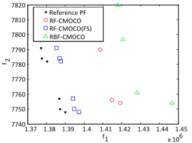
As shown in Fig. 11, the solution set obtained by RF-CMOCO(FS) is still much worse than the reference PF. Note that the computation time consumed for obtaining the reference PF and that for the compared algorithms that use a maximum of 2000 exact function evaluations are different, as detailed in Table VI. It takes about 56 hours for the NSGA-II to
1.37 1.38 1.39 1.4 1.41 1.42 1.43 1.44 1.45 x 10⁶ 7740 7750 7760 7770 7780 7790 7800 7810 7820 f1 f 2 Reference PF RF-CMOCO RF-CMOCO(FS) RBF-CMOCO
Fig. 11. Non-dominated solution set of the Colorado trauma system design problem obtained by RF-CMOCO, RF-CMOCO(FS), and RBF-CMOCO using 2000 exact function evaluations.
obtain the reference PF. By contrast, the compared algorithms consume only about 3 hours to obtain the results. Therefore, RF-CMOCO(FS) is still very competitive taking into account the fact that it consumes much less computation time than NSGA-II.
TABLE VI
THE AVERAGE RUNTIME(H)OFNSGA-II (FOR OBTAINING THE
REFERENCEPF), RF-CMOCO, RF-CMOCO(FS), RBF-CMOCO,AND
NSGA-II (USING A MAXIMUM OF2000EXACT FUNCTION EVALUATIONS)
ONCOLORADO TRAUMA SYSTEM DESIGN PROBLEM.
NSGA-II for reference PF 55.85 RF-CMOCO 3.21 RF-CMOCO(FS) 3.36 RBF-CMOCO 3.34
NSGA-II 2.73
From the two different trauma system design problems, we can conclude that RF-CMOCO is effective for solving expensive data-driven combinatorial optimization problems. Based on the comparative results, we can also conclude that the RF models are better suited as surrogates for combinatorial optimization problems than the RBF models. Finally, the results demonstrate that dimension reduction techniques such as feature selection are able to enhance the performance of RF-assisted EAs for solving high-dimensional combinatorial optimization problems.
V. CONCLUDINGREMARKS
In this paper, we present a random forest assisted evo-lutionary algorithm for solving expensive data-driven con-strained multi-objective combinatorial optimization problems. We show that random forest models work better than radial-basis-function network models as surrogates for combinatorial optimization problems. To address the errors introduced by the surrogates for the constraints, we design a correction boundary strategy with the help of logistic regression models and a stochastic ranking strategy using two selection criteria, one considering the problem as an unconstrained multi-objective problem and the other as a constrained multi-objective prob-lem. Our empirical results demonstrate that the proposed
constraint handling strategies based on logistic regression correction and stochastic ranking can improve the selection accuracy up to 70%-80% in the optimization process. The effectiveness of the RF-CMOCO has been verified on both multi-objective knapsack problems and two real-world data-driven trauma system design problems.
Although the effectiveness and efficiency of the proposed algorithms are promising in that they can significantly reduce the computation time at the price of slight quality degradation, some open issues remain to be resolved in the future. First, there is much room for improving the performance of random forest models, and better surrogate models for approximating the objective and constraint functions are in high demand. Second, indirect surrogate models for permutation or tree structures need to be studied so that surrogate-assisted evo-lutionary algorithms can be applied to a wider range of com-binatorial optimization problems. Finally, more sophisticated machine learning techniques are required to determine whether a solution is feasible or not, which heavily influences the performance of surrogate-assisted evolutionary optimization of expensive constrained problems.
ACKNOWLEDGEMENT
The authors would like to thank Dr Jan O Jansen, Dr Ernest E Moore, Dr Jonathan J Morrison, Dr James D Hutchison, and Dr Marion K Campbell for providing the data of the Colorado trauma system problem.
REFERENCES
[1] K. L. Hoffman, “Combinatorial optimization: Current successes and directions for the future,”Journal of computational and applied mathe-matics, vol. 124, no. 1, pp. 341–360, 2000.
[2] M. Ehrgott and X. Gandibleux, “A survey and annotated bibliography of multiobjective combinatorial optimization,”OR Spectrum, vol. 22, no. 4, pp. 425–460, 2000.
[3] K. Florios, G. Mavrotas, and D. Diakoulaki, “Solving multiobjective, multiconstraint knapsack problems using mathematical programming and evolutionary algorithms,” European Journal of Operational Re-search, vol. 203, no. 1, pp. 14–21, 2010.
[4] Y. Jin, “A comprehensive survey of fitness approximation in evolutionary computation,”Soft Computing, vol. 9, no. 1, pp. 3–12, 2005. [5] H. Wang, Y. Jin, and J. O. Janson, “Data-driven surrogate-assisted
multi-objective evolutionary optimization of a trauma system,” IEEE Transactions on Evolutionary Computation, vol. 20, no. 6, pp. 939–952, 2016.
[6] Y. Jin, “Surrogate-assisted evolutionary computation: Recent advances and future challenges,”Swarm and Evolutionary Computation, vol. 1, no. 2, pp. 61–70, 2011.
[7] Y. Jin and B. Sendhoff, “A systems approach to evolutionary mul-tiobjective structural optimization and beyond,” IEEE Computational Intelligence Magazine, vol. 4, no. 3, pp. 62–76, 2009.
[8] H. Wang, J. Doherty, and Y. Jin, “Hierarchical surrogate-assisted evo-lutionary multi-scenario airfoil shape optimization,” inProceedings of the 2018 IEEE World Congress on Computational Intelligence (WCCI 2018). IEEE, 2018.
[9] S. Koziel and A. Bekasiewicz, “Rapid simulation-driven multiobjective design optimization of decomposable compact microwave passives,” IEEE Transactions on Microwave Theory and Techniques, vol. 64, no. 8, pp. 2454–2461, 2016.
[10] D. Guo, T. Chai, J. Ding, and Y. Jin, “Small data driven evolutionary multi-objective optimization of fused magnesium furnaces,” in IEEE Symposium Series on Computational Intelligence. Athens, Greece: IEEE, December 2016.
[11] B. Liu, Q. Zhang, and G. G. Gielen, “A Gaussian process surrogate model assisted evolutionary algorithm for medium scale expensive opti-mization problems,” IEEE Transactions on Evolutionary Computation, vol. 18, no. 2, pp. 180–192, 2014.
[12] R. Allmendinger, M. T. M. Emmerich, J. Hakanen, Y. Jin, and E. Rigoni, “Surrogate-assisted multicriteria optimization: Complexities, prospective solutions, and business case,”Journal of Multi-Criteria Decision Anal-ysis, vol. 14, pp. 5–25, 2017.
[13] T. Chugh, Y. Jin, K. Miettinen, J. Hakanen, and K. Sindhya, “A surrogate-assisted reference vector guided evolutionary algorithm for computationally expensive many-objective optimization,”IEEE Trans-actions on Evolutionary Computation, vol. 22, no. 1, pp. 129–142, 2018. [14] L. Willmes, T. Back, Y. Jin, and B. Sendhoff, “Comparing neural networks and kriging for fitness approximation in evolutionary optimiza-tion,” inIEEE Congress on Evolutionary Computation, vol. 1. IEEE, 2003, pp. 663–670.
[15] R. G. Regis, “Evolutionary programming for high-dimensional con-strained expensive black-box optimization using radial basis functions,” IEEE Transactions on Evolutionary Computation, vol. 18, no. 3, pp. 326–347, 2014.
[16] C. Sun, Y. Jin, J. Zeng, and Y. Yu, “A two-layer surrogate-assisted particle swarm optimization algorithm,”Soft Computing, vol. 19, no. 6, pp. 1461–1475, 2015.
[17] Z. Zhou, Y. S. Ong, P. B. Nair, A. J. Keane, and K. Y. Lum, “Combining global and local surrogate models to accelerate evolutionary optimiza-tion,”IEEE Transactions on Systems, Man, and Cybernetics, Part C: Applications and Reviews, vol. 37, no. 1, pp. 66–76, 2007.
[18] H. Wang, Y. Jin, C. Sun, and J. Doherty, “Offline data-driven evolutionary optimization using selective surrogate ensembles,” IEEE Transactions on Evolutionary Computation, 2018, accepted, DOI=0.1109/TEVC.2018.2834881.
[19] Z. Zhou, Y. S. Ong, M. H. Nguyen, and D. Lim, “A study on polynomial regression and Gaussian process global surrogate model in hierarchical surrogate-assisted evolutionary algorithm,” inIEEE Congress on Evolu-tionary Computation, vol. 3. IEEE, 2005, pp. 2832–2839.
[20] Y. Jin, M. Olhofer, and B. Sendhoff, “A framework for evolutionary optimization with approximate fitness functions,”IEEE Transactions on Evolutionary Computation, vol. 6, no. 5, pp. 481–494, 2002. [21] M. H¨usken, Y. Jin, and B. Sendhoff, “Structure optimization of neural
networks for evolutionary design optimization,”Soft Computing, vol. 9, no. 1, pp. 21–28, 2005.
[22] D. Lim, Y. Jin, Y.-S. Ong, and B. Sendhoff, “Generalizing surrogate-assisted evolutionary computation,”IEEE Transactions on Evolutionary Computation, vol. 14, no. 3, pp. 329–355, 2010.
[23] A. Husain and K.-Y. Kim, “Enhanced multi-objective optimization of a microchannel heat sink through evolutionary algorithm coupled with multiple surrogate models,” Applied Thermal Engineering, vol. 30, no. 13, pp. 1683–1691, 2010.
[24] D. Lim, Y.-S. Ong, Y. Jin, and B. Sendhoff, “A study on metamodeling techniques, ensembles, and multi-surrogates in evolutionary computa-tion,” in Proceedings of the 9th Annual Conference on Genetic and Evolutionary Computation. ACM, 2007, pp. 1288–1295.
[25] H. Wang, Y. Jin, and J. Doherty, “Committee-based active learning for surrogate-assisted particle swarm optimization of expensive problems,” IEEE Transactions on Cybernetics, vol. 47, no. 9, pp. 2664–2677, 2017. [26] Y. Jin, M. Olhofer, and B. Sendhoff, “On evolutionary optimization with approximate fitness functions,” inProceedings of the 2nd Annual Con-ference on Genetic and Evolutionary Computation. Morgan Kaufmann Publishers Inc., 2000, pp. 786–793.
[27] J. Branke and C. Schmidt, “Faster convergence by means of fitness estimation,”Soft Computing, vol. 9, no. 1, pp. 13–20, 2005.
[28] M. T. Emmerich, K. C. Giannakoglou, and B. Naujoks, “Single-and multiobjective evolutionary optimization assisted by gaussian random field metamodels,” IEEE Transactions on Evolutionary Computation, vol. 10, no. 4, pp. 421–439, 2006.
[29] Y. S. Ong, P. B. Nair, and A. J. Keane, “Evolutionary optimization of computationally expensive problems via surrogate modeling,”AIAA journal, vol. 41, no. 4, pp. 687–696, 2003.
[30] C. Sun, Y. Jin, R. Cheng, J. Ding, and J. Zeng, “Surrogate-assisted co-operative swarm optimization of high-dimensional expensive problems,” IEEE Transactions on Evolutionary Computation, vol. 21, no. 4, pp. 644–660, 2017.
[31] J. Knowles, “ParEGO: a hybrid algorithm with on-line landscape ap-proximation for expensive multiobjective optimization problems,”IEEE Transactions on Evolutionary Computation, vol. 10, no. 1, pp. 50–66, 2006.
[32] Q. Zhang, W. Liu, E. Tsang, and B. Virginas, “Expensive multiobjective optimization by MOEA/D with gaussian process model,”IEEE Transac-tions on Evolutionary Computation, vol. 14, no. 3, pp. 456–474, 2010.
[33] L. Pan, C. He, Y. Tian, H. Wang, X. Zhang, and Y. Jin, “A classification based surrogate-assisted evolutionary algorithm for expensive many-objective optimization,”IEEE Transactions on Evolutionary Computa-tion, 2018, accepted, DOI=10.1109/TEVC.2018.2802784.
[34] T. Bartz-Beielstein and M. Zaefferer, “Model-based methods for contin-uous and discrete global optimization,”Applied Soft Computing, vol. 55, pp. 154–167, 2017.
[35] F. Hutter, H. H. Hoos, and K. Leyton-Brown, “Sequential model-based optimization for general algorithm configuration.”LION, vol. 5, pp. 507– 523, 2011.
[36] R. Li, M. Emmerich, J. Eggermont, and E. Bovenkamp, “Mixed-integer optimization of coronary vessel image analysis using evolution strategies,” inProceedings of the 8th Annual Conference on Genetic and Evolutionary Computation, 2006, pp. 1645–1652.
[37] L. Zhuang, K. Tang, and Y. Jin, “Metamodel assisted mixed-integer evolution strategies based on kendall rank correlation coefficient,” in In-ternational Conference on Intelligent Data Engineering and Automated Learning. Springer, 2013, pp. 366–375.
[38] A. Moraglio and A. Kattan, “Geometric generalisation of surrogate model based optimisation to combinatorial spaces,” inEuropean Con-ference on Evolutionary Computation in Combinatorial Optimization. Springer, 2011, pp. 142–154.
[39] R. van der Merwe, T. K. Leen, Z. Lu, S. Frolov, and A. M. Baptista, “Fast neural network surrogates for very high dimensional physics-based models in computational oceanography,”Neural Networks, vol. 20, no. 4, pp. 462–478, 2007.
[40] D.-J. Wang, F. Liu, Y.-Z. Wang, and Y. Jin, “A knowledge-based evolutionary proactive scheduling approach in the presence of machine breakdown and deterioration effect,”Knowledge-Based Systems, vol. 90, pp. 70–80, 2015.
[41] S. Nguyen, M. Zhang, and K. C. Tan, “Surrogate-assisted genetic pro-gramming with simplified models for automated design of dispatching rules,”IEEE transactions on cybernetics, vol. 47, no. 9, pp. 2951–2965, 2017.
[42] I. Voutchkov, A. Keane, A. Bhaskar, and T. M. Olsen, “Weld se-quence optimization: the use of surrogate models for solving sequential combinatorial problems,”Computer methods in applied mechanics and engineering, vol. 194, no. 30, pp. 3535–3551, 2005.
[43] B. Yuan, B. Li, T. Weise, and X. Yao, “A new memetic algorithm with fitness approximation for the defect-tolerant logic mapping in crossbar-based nanoarchitectures,”IEEE Transactions on Evolutionary Computation, vol. 18, no. 6, pp. 846–859, 2014.
[44] Z. Cai and Y. Wang, “A multiobjective optimization-based evolutionary algorithm for constrained optimization,”IEEE Transactions on Evolu-tionary Computation, vol. 10, no. 6, pp. 658–675, 2006.
[45] M. Kazemi, G. G. Wang, S. Rahnamayan, and K. Gupta, “Metamodel-based optimization for problems with expensive objective and constraint functions,”Journal of Mechanical Design, vol. 133, no. 1, p. 014505, 2011.
[46] K. S. Won and T. Ray, “A framework for design optimization using surrogates,” Engineering Optimization, vol. 37, no. 7, pp. 685–703, 2005.
[47] C. A. C. Coello, “Theoretical and numerical constraint-handling tech-niques used with evolutionary algorithms: a survey of the state of the art,”Computer methods in applied mechanics and engineering, vol. 191, no. 11, pp. 1245–1287, 2002.
[48] H. K. Singh, T. Ray, and W. Smith, “Surrogate assisted simulated annealing (SASA) for constrained multi-objective optimization,” inIEEE Congress on Evolutionary Computation. IEEE, 2010, pp. 1–8. [49] J. M. Parr, A. I. Forrester, A. J. Keane, and C. M. Holden, “Enhancing
infill sampling criteria for surrogate-based constrained optimization,” Journal of Computational Methods in Sciences and Engineering, vol. 12, no. 1, 2, pp. 25–45, 2012.
[50] J. Poloczek and O. Kramer, “Local SVM constraint surrogate models for self-adaptive evolution strategies,” inAnnual Conference on Artificial Intelligence. Springer, 2013, pp. 164–175.
[51] S. D. Handoko, C. K. Kwoh, and Y.-S. Ong, “Feasibility structure modeling: an effective chaperone for constrained memetic algorithms,” IEEE Transactions on Evolutionary Computation, vol. 14, no. 5, pp. 740–758, 2010.
[52] Y. Tenne, K. Izui, and S. Nishiwaki, “Handling undefined vectors in expensive optimization problems,” in European Conference on the Applications of Evolutionary Computation. Springer, 2010, pp. 582– 591.
[53] O. Kramer, A. Barthelmes, and G. Rudolph, “Surrogate constraint functions for CMA evolution strategies,” in Annual Conference on Artificial Intelligence. Springer, 2009, pp. 169–176.