Tahani Muqbil Alqurashi
A thesis submitted in fulfilment
of the requirements for the degree of
Doctor of Philosophy
School of Computing Sciences
University of East Anglia
January, 2017
c
This copy of the thesis has been supplied on condition that anyone who consults it is understood to recognise that its copyright rests with the author and that use of any information derived
there-Clustering is an unsupervised learning paradigm that partitions a given dataset into clusters so that objects in the same cluster are more similar to each other than to the objects in the other clusters. However, when clustering algorithms are used individ-ually, their results are often inconsistent and unreliable. This research applies the philosophy of Ensemble learning that combines multiple partitions using a consensus function in order to address these issues to improve a clustering performance.
A clustering ensemble framework is presented consisting of three phases: En-semble Member Generation, Consensus and Evaluation. This research focuses on two points: the consensus function and ensemble diversity. For the first, we pro-posed three new consensus functions: the Object-Neighbourhood Clustering Ensem-ble (ONCE), the Dual-Similarity Clustering EnsemEnsem-ble (DSCE), and the Adaptive Clustering Ensemble (ACE). ONCE takes into account the neighbourhood relation-ship between object pairs in the similarity matrix, while DSCE and ACE are based on two similarity measures: cluster similarity and membership similarity.
The proposed ensemble methods were tested on benchmark real-world and arti-ficial datasets. The results demonstrated that ONCE outperforms the other similar methods, and is more consistent and reliable than k-means. Furthermore, DSCE and ACE were compared to the ONCE, CO, MCLA and DICLENS clustering en-semble methods. The results demonstrated that on average ACE outperforms the state-of-the-art clustering ensemble methods, which are CO, MCLA and DICLENS.
On diversity, we experimentally investigated all the existing measures for deter-mining their relationship with the ensemble quality. The results indicate that none
members, and (2) none of them have been used directly by any consensus function. Therefore, we point out that these two issues need to be addressed in future research.
Some of the results presented in this thesis has been reported in the following pub-lications:
Journal Papers
• Tahani Alqurashi and Wenjia Wang. A novel adaptive clustering ensemble method. International Journal of Machine Learning and Cybernetics, Springer, 2016. Note: Accepted subject to minor revision.
Conference Papers
• Tahani Alqurashi and Wenjia Wang. Object-neighbourhood clustering ensemble method. In Proceedings of the Intelligent Data Engineering and Automated Learning (IDEAL), pages 142−149. Springer, 2014.
• Tahani Alqurashi and Wenjia Wang. A new consensus function based on dual-similarity measurements for clustering ensemble. In Proceedings of the International Conference on Data Science and Advanced Analytics (DSAA), pages 149−155. IEEE/ACM, 2015.
Other Publication
• Tahani Alqurashi and Wenjia Wang. A Graph based Methodology for Web Structure Mining-with a Case Study on the Webs of UK Universities. In Proceedings of the 4th Inter-national Conference on Web Intelligence, Mining and Semantics (WIMS), page 4. ACM, 2014.
First and foremost, I would like to thank Almighty Lord, who has made everything possible. A special thanks goes to Dr Wenjia Wang, who was not only my super-visor but also my mentor. He has been supportive since my Masters degree and throughout the long road to the end of my thesis. He gave me confidence in my work and was always present for guidance and help whenever I needed it. Thank you Wenjia, for giving me the opportunity to work with you. And big thanks go to all the staff in the Computing Sciences School — it was a great honour to work with you. I also would like to thank the reviewers of my papers for their critical comments and suggestions.
This thesis is also the result of many people who supported me emotionally: Mum and Dad, thanks for your support, which helped me to overcome my fears and thank you for encouraging me to achieve my dreams. Thanks for being a role model to me. Yaser, you are the source of endless love and kindness, your love helped me overcome difficult times. Thank you for being my best friend, and a supportive husband. Sultan and Yasmin, you are the best kids I could ask for, thank you for your patience and I know you both suffered so much during my study for not having the time you needed. My sisters and brothers, I wish I were with you during the last four years. I thank you for believing in me and I hope I made you proud of your sister.
Lastly, I would like to show my deepest gratitude to my sponsor, Umm Al-Qura University and the Ministry of Education in Saudi Arabia, for the full scholarship
List of Figures ix
List of Tables xv
List of Abbreviations xviii
1 Introduction 3
1.1 Background . . . 3
1.2 Research Motivation . . . 4
1.2.1 Consensus Function . . . 5
1.2.2 Clustering Ensemble Diversity . . . 6
1.3 Research Questions . . . 7 1.4 Thesis Organisation . . . 7 2 Literature Review 10 2.1 Clustering Methods . . . 10 2.1.1 Hierarchical Clustering . . . 12 2.1.2 Partition Clustering . . . 13 2.1.3 Fuzzy Clustering . . . 15
2.1.4 Issues with Clustering Algorithms . . . 15
2.2 Clustering Ensemble Methods . . . 16
2.2.1 The Process of the Clustering Ensemble Method . . . 17
2.2.2 Ensemble Generation Techniques . . . 18
2.2.3 Review of Consensus Functions . . . 20
2.2.3.1 Graph-based Methods . . . 22
2.2.3.2 Object Pairwise Similarity-based Methods . . . 24
2.2.3.4 Probability-based Methods . . . 27
2.2.3.5 Link-based Methods . . . 29
2.2.4 Clustering Ensemble Evaluation . . . 32
2.2.4.1 External Validation Index . . . 32
2.2.4.2 Internal Validation Index . . . 35
2.2.4.3 Relative Validation Index . . . 38
2.3 Clustering Ensemble Diversity . . . 39
2.3.1 Related Work on Clustering Ensemble Diversity Measures . . 40
2.3.1.1 Pairwise Diversity Measure (p) . . . 40
2.3.1.2 Non-Pairwise Diversity Measures (np) . . . 42
2.3.2 The Relationship between Diversity and Ensemble . . . 43
2.4 Clustering Ensemble Application . . . 46
2.5 Summary . . . 47
3 Research Methodology 49 3.1 The Clustering Ensemble Framework . . . 49
3.2 Strategies to Test the Effectiveness of the Proposed Consensus Func-tions . . . 52
3.2.1 Dataset . . . 53
3.2.2 Ensemble Member Generation Techniques Used . . . 54
3.2.3 Comparison Strategy . . . 56
3.2.4 Evaluation Measures Used . . . 57
3.2.5 Tests of Statistical Significance . . . 57
3.3 Strategies Used to Investigate Diversity . . . 59
3.3.1 Analysis of the Positive and Negative Effects of Diversity on the Ensemble Performance . . . 60
3.3.2 Studying the Interaction between Members’ Qualities and Di-versity . . . 60
3.4 Research Tools and Implementation . . . 62
3.5 Summary . . . 64
4 Object-Neighbourhood Clustering Ensemble 65 4.1 Object-Neighbourhood Clustering Ensemble . . . 66
4.1.3 Illustrative Example . . . 69
4.1.4 Experimental Results . . . 73
4.2 E-Object Neighbourhood Clustering Ensemble . . . 79
4.2.1 Definition ofE-Object Neighbourhood Similarity (E-ONCE) . 79 4.2.2 Experimental Results . . . 80
4.3 Comparing ONCE with other Consensus Functions . . . 83
4.3.1 Experimental Results . . . 83
4.3.2 Comparing ONCE with Individual Members . . . 86
4.3.3 Test of Significance . . . 87
4.4 Summary . . . 88
5 Adaptive Clustering Ensemble 91 5.1 Dual-Similarity Clustering Ensemble (DSCE) . . . 92
5.1.1 Definitions and Notations . . . 95
5.1.2 The DSCE Algorithm . . . 97
5.1.3 An Illustrative Example . . . 102
5.1.4 Experimental Design . . . 107
5.1.5 Experimental Results . . . 107
5.1.6 Test of Significance . . . 110
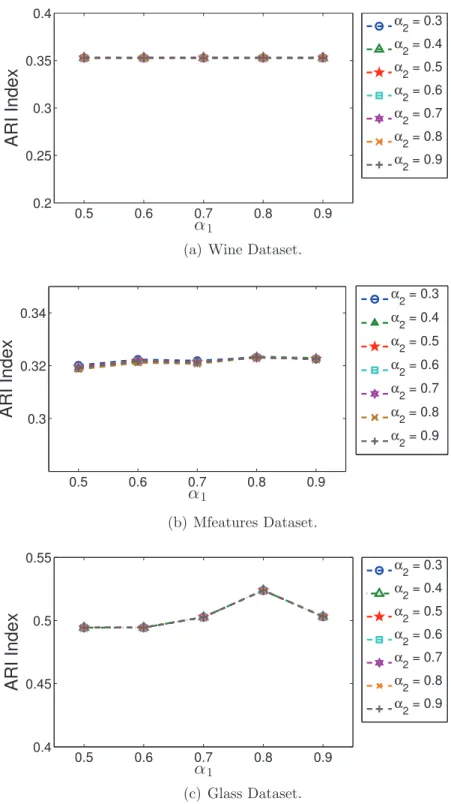
5.1.7 Analysis of Parameters and Time Complexity . . . 112
5.2 The Adaptive Clustering Ensemble (ACE) . . . 115
5.2.1 The ACE Algorithm . . . 115
5.2.2 An illustrative Example . . . 124
5.2.3 Experimental Design . . . 127
5.2.4 Experimental Results . . . 128
5.2.4.1 Results of Ensembles Built with Fixed k . . . 128
5.2.4.2 Results of Ensembles Built with Random Variable k 130 5.2.5 Test of Significance . . . 133
5.2.6 Analysis of Parameters and Time Complexity . . . 134
5.3 Summary . . . 139
6 The Diversity of the Clustering Ensemble. 141 6.1 Experimental Studies on Clustering Ensemble Diversity . . . 142
6.1.2 Experimental Results . . . 143
6.1.3 Studying the Correlation between the Ensemble Performance and the Diversity. . . 155
6.2 Investigation of Issues Raised . . . 156
6.2.1 Analysis of the Positive and Negative Effects of Diversity on the Ensemble Performance . . . 157
6.2.1.1 Experimental Design . . . 158
6.2.1.2 Summary of Results . . . 160
6.2.1.3 The Experiment of Eliminating Poor Members . . . 162
6.2.2 The Experimental Study of the Interaction between Members’ Qualities and Diversity . . . 168
6.2.2.1 Experimental Results . . . 170
6.2.2.2 Result of ANOVA . . . 173
6.2.2.3 Summary of Results . . . 177
6.3 Discussion . . . 179
6.3.1 Discussion on the Issues Raised in our Diversity Studies . . . . 183
6.3.2 General Discussion on Diversity . . . 187
6.4 Summary . . . 188
7 Conclusions and Further Work 191 7.1 Conclusions . . . 191
7.1.1 On the Consensus Function . . . 191
7.1.2 On Diversity . . . 193
7.1.3 Contributions . . . 196
7.2 Suggestions for Further Work . . . 197
Appendix A 199 A.1 The Statistical Summary of the Results . . . 199
A.2 Demonstrating Results in Boxplots . . . 200
A.3 Demonstrating Results in Line Charts . . . 205
Appendix B 239 B.1 The Complete Results of Analysis of the Positive and Negative Effects of Diversity . . . 239
Appendix C 278
2.1 The Clustering Ensemble Process [102] . . . 18 2.2 Diagram of the five categories of the ensemble generation techniques,
as classified by Iam-on et al. [48]. . . 21 2.3 The two categories of diversity measures that have been proposed in
the literature and the subdivision of the Non-Pairwise measure. . . . 41
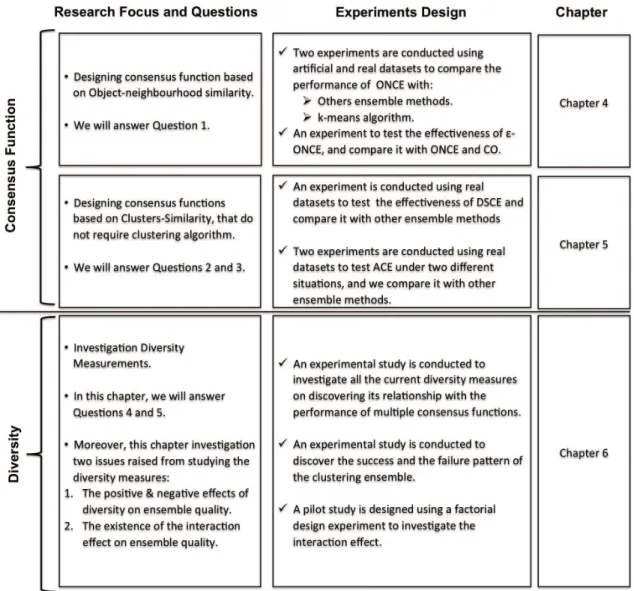
3.1 A Clustering Ensemble Framework. . . 50 3.2 Summary of the thesis experimental chapters. . . 53 3.3 Three artificial datasets are used in this study. The number of clusters
is given in parentheses. . . 55
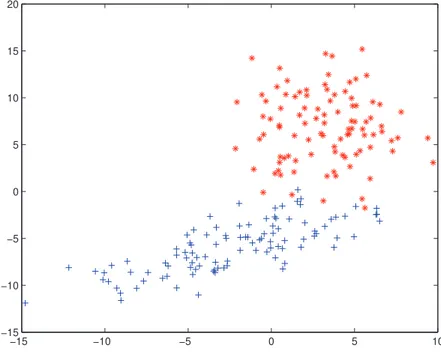
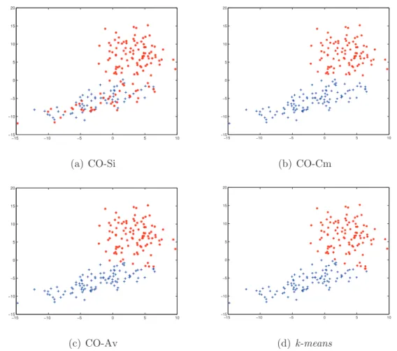
4.1 The different types of objects pairs and their similarity value. . . 67 4.2 The generated artificial dataset consists of 2 clusters and 200 objects. 71 4.3 The Cluster labels results of CO-Si, CO-Cm, CO-Av, E-ONCE-Cm
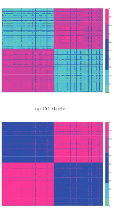
clustering ensemble methods andk-means algorithm. . . 73 4.4 The heat map of the CO and ONCE matrices calculated using the
artificial dataset. . . 74 4.5 The Critical difference diagram of the critical level of 0.1 in which
it shows the comparison of five ensemble methods using 11 datasets. The original quality results of these methods are shown in table 4.7. . 88
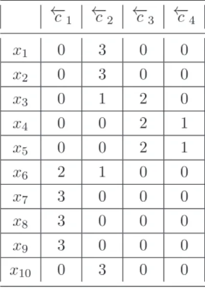
5.1 The DSCE flow chart. . . 94 5.2 An illustrative example of three clustering members for dataset X
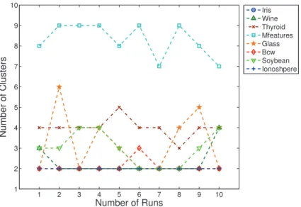
of 10 objects, and the transformation from members into a binary vectors representation. . . 103 5.3 Number of clusters produced by DSCE algorithm for each dataset in
ten runs. The true number of clusters for{Iris, Wine, Thyroid} = 3, Mfeatuers = 10, Glass = 6, Bcw = 2, Soybean = 4, Ionosphere = 2. . 110
5.4 Number of clusters produced by DICLENS algorithm for each dataset in ten runs. The true number of clusters for{Iris, Wine, Thyroid} = 3, Mfeatuers = 10, Glass = 6, Bcw = 2, Soybean = 4, Ionosphere = 2.111 5.5 The critical difference diagram at the critical level of 0.1. It shows
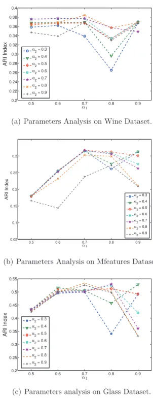
the comparison of four ensemble methods using 8 datasets. . . 112 5.6 The Average ARI index of ten runs for analysing the two parameters
α1 and α2. . . 114
5.7 The diagram of the ACE algorithm . . . 116 5.8 Number of clusters produced by DICLENS algorithm for each dataset
in ten runs for the result in the second experiment. The true number of clusters for {Iris, Wine, Thyroid} = 3, Mfeatures= 10, Glass = 6, Bcw = 2, Soybean = 4, Ionosphere = 2. . . 133 5.9 The Critical difference diagram of the critical level of 0.1 in which it
shows the comparison of six ensemble methods using eight datasets. . 134 5.10 The Average of ARI index of ten runs for analysing the two
parame-ters α1 and α2 using members with fixed k. . . 137
5.11 The Average of ARI index of ten runs for analysing the two parame-ters α1 and α2 using members with random k. . . 138
6.1 TheDVpN M I,DVnp1 and DVnp4 measures from Bcw dataset. (a), (b)
and (c) using MCLA, while (d), (e) and (f) using ONCE-Av. . . 145 6.2 The DVpARI, DVnp2 and DVnp4 measures from Ionosphere dataset
(a),(b) and (c) using CO-Av., while (d), (e) and (f) using MCLA. . . 146 6.3 The DVpARI, DVnp3 and DVnp4 measures from Iris dataset, (a), (b)
and (c) using CO-Av, while (d), (e) and (f) using MCLA. . . 147 6.4 TheDVpARI, DVnp1 andDVnp3 measures from Soybean dataset , (a),
(b) and (c) using CO-Av, while (d), (e) and (f) using ACE. . . 148 6.5 The DVpARI and DVnp3 measures from Thyroid dataset, (a) and (b)
using CO-Ave, while (c) and (d) using ONCE-Av. . . 149 6.6 The DVnp1 and DVnp3 measures from Thyroid dataset, (a) and (b)
using MCLA, while (c) and (d) using ACE. . . 150 6.7 The DVpARI, DVnp1, DVnp3 and DVnp4 measures from Wine dataset
using ACE. . . 151 6.8 TheEntropy,DVnp1 and DVnp3 measures from Glass dataset,(a), (b)
and (c) using CO-Ave, while (d), (e) and (f) using MCLA. . . 152 6.9 TheDVpARI,DVnp1 and DVnp3 measures from Mfeatures dataset (a),
(b) and (c) using CO-Ave, while (d), (e) and (f) using MCLA. . . 153 6.10 The Number of members whose Poor, Good and Medium Q-mem
6.11 25 ensemble runs for case 1 & 2, in each run one member is removed. 164 6.12 25 ensemble runs for case 7 & 8, in each run one member is removed. 164 6.13 25 ensemble runs for case 13 & 14, in each run one member is removed.165 6.14 25 ensemble runs for case 15 &16, in each run one member is removed.165 6.15 25 ensemble runs for case 17 & 18, in each run one member is removed.166 6.16 25 ensemble runs for case 9 & 10, in each run one member is removed. 166 6.17 The range values of the member quality and the ensemble diversity,
including the interaction area between them. . . 169 6.18 The main effects of the diversity and member quality on the response
variables, which are CO, ONCE, ACE and MCLA, for Thyroid dataset.172 6.19 The main effects of the diversity and member quality on the response
variables, which are CO, ONCE, ACE and MCLA, for Wine dataset. 172 6.20 The interaction effects of the diversity and member quality on the
re-sponse variables, which are CO, ONCE, ACE and MCLA, for Thyroid dataset. . . 174 6.21 The interaction effects of the diversity and member quality on the
response variables, which are CO, ONCE, ACE and MCLA, for Wine dataset. . . 174 6.22 The Tukey results with Wine dataset using the ACE and MCLA. The
Tukey test used to determine specifically which means are statistically significant different of the interaction effects using these consensus functions. . . 178
A.1 The boxplot of the diversity results measured by the pairwise diversity measures: it shows the distribution of the diversity values of generated members in 100 runs in the 8 tested datasets. The line in each box represent the median value of the diversity and the star represents the mean value of 100 runs. . . 202 A.2 The boxplot of the diversity results measured by the non-pairwise
diversity measures using CO and ONCE methods. . . 203 A.3 The boxplot of the diversity results measured by the non-pairwise
diversity measures using ACE and MCLA methods. . . 204 A.4 The seven diversity measures from Iris dataset using CO-Av. . . 206 A.5 The seven diversity measures from Iris dataset using ONCE-Av. . . . 207 A.6 The seven diversity measures from Iris dataset using ACE. . . 208 A.7 The seven diversity measures from Iris dataset using MCLA. . . 209 A.8 The seven diversity measures from Wine dataset using CO-Av. . . . 210
A.10 The seven diversity measures from Wine dataset using MCLA. . . 212 A.11 The seven diversity measures from Wine dataset using ACE. . . 213 A.12 The seven diversity measures from Glass dataset using CO-Av. . . 214 A.13 The seven diversity measures from Glass dataset using ONCE-Av. . . 215 A.14 The seven diversity measures from Glass dataset using MCLA. . . 216 A.15 The seven diversity measures from Glass dataset using ACE. . . 217 A.16 The seven diversity measures from Thyroid dataset using CO-Av. . . 218 A.17 The seven diversity measures from Thyroid dataset using ONCE-Av. 219 A.18 The seven diversity measures from Thyroid dataset using MCLA. . . 220 A.19 The seven diversity measures from Thyroid dataset using ACE. . . . 221 A.20 The seven diversity measures from Mfeatures dataset using CO-Av. . 222 A.21 The seven diversity measures from Mfeatures dataset using ONCE-Av.223 A.22 The seven diversity measures from Mfeatures dataset using MCLA. . 224 A.23 The seven diversity measures from Mfeatures dataset using ACE. . . 225 A.24 The seven diversity measures from Bcw dataset using CO-Av. . . 226 A.25 The seven diversity measures from Bcw dataset using ONCE-Av. . . 227 A.26 The seven diversity measures from Bcw dataset using MCLA. . . 228 A.27 The seven diversity measures from Bcw dataset using ACE. . . 229 A.28 The seven diversity measures from Soybean dataset using CO-Av. . . 230 A.29 The seven diversity measures from Soybean dataset using ONCE-Av. 231 A.30 The seven diversity measures from Soybean dataset using MCLA. . . 232 A.31 The seven diversity measures from Soybean dataset using ACE. . . . 233 A.32 The seven diversity measures from Ionosphere dataset using CO-Av. . 234 A.33 The seven diversity measures from Ionosphere dataset using
ONCE-Av. . . 235 A.34 The seven diversity measures from Ionosphere dataset using MCLA. . 236 A.35 The seven diversity measures from Ionosphere dataset using ACE. . . 237
B.1 Pair # 1 consists of Case 1 and Case 2. . . 244 B.2 The heat map of the CO similarity matrix for Case 1 and Case 2. . . 245 B.3 The heat map of the ONCE similarity matrix for Case 1 and Case 2. 246 B.4 The heat map of the true label of the Thyroid dataset. . . 247 B.5 Pair # 2 consists of Case 3 and Case 4. . . 248 B.6 Pair # 3 consists of Case 5 and Case 6. . . 249
B.7 Pair # 4 consists of Case 7 and Case 8. . . 250
B.8 The heat map of the CO similarity matrix for Case 7 and Case 8. . . 251
B.9 Pair # 5 consists of Case 9 and Case 10. . . 252
B.10 Pair # 6 consists of Case 11 and Case 12. . . 253
B.11 Pair # 7 consists of Case 13 and Case 14. . . 254
B.12 Pair # 8 consists of Case 15 and Case 16. . . 255
B.13 Pair # 9 consists of Case 17 and Case 18. . . 256
B.14 Pair # 10 consists of Case 19 and Case 20. . . 257
B.15 Pair # 11 consists of Case 21 and Case 22. . . 258
B.16 Pair #1 consists of Case 1 and Case 2. . . 259
B.17 Pair #2 consists of Case 3 and Case 4. . . 259
B.18 Pair #3 consists of Case 5 and Case 6. . . 260
B.19 Pair #4 consists of Case 7 and Case 8. . . 260
B.20 Pair #5 consists of Case 9 and Case 10. . . 261
B.21 Pair #6 consists of Case 11 and Case 12. . . 261
B.22 Pair #7 consists of Case 13 and Case 14. . . 262
B.23 Pair #8 consists of Case 15 and Case 16. . . 262
B.24 Pair #9 consists of Case 17 and Case 18. . . 263
B.25 Pair #10 consists of Case 19 and Case 20. . . 263
B.26 Pair #11 consists of Case 21 and Case 22. . . 264 B.27 25 ensemble runs for case 1 & 2, in each run one member is removed. 270 B.28 25 ensemble runs for case 3 & 4, in each run one member is removed. 271 B.29 25 ensemble runs for case 5 & 6, in each run one member is removed. 271 B.30 25 ensemble runs for case 7 & 8, in each run one member is removed. 272 B.31 25 ensemble runs for case 9 & 10, in each run one member is removed. 272 B.32 25 ensemble runs for case 11 & 12, in each run one member is removed.273 B.33 25 ensemble runs for case 13 & 14, in each run one member is removed.273 B.34 25 ensemble runs for case 15 &16, in each run one member is removed.274 B.35 25 ensemble runs for case 17 & 18, in each run one member is removed.274 B.36 25 ensemble runs for case 19 & 20, in each run one member is removed275 B.37 25 ensemble runs for case 21 & 22, in each run one member is removed275 B.38 The heat map of the CO similarity matrix for Run 7 at case 7 and 8. 276
B.40 The heat map of the CO similarity matrix for Run 7 and 10 at case 15.276 B.41 The heat map of the ONCE similarity matrix for Run 2 and 7 at case
15. . . 277
C.1 The normal probability plot of the response variables (CO, ONCE, ACE and MCLA) for Thyroid dataset. . . 279 C.2 The normal probability plot of the response variables (CO, ONCE,
2.1 Summary of diversity research proposed in the literature for discov-ering the relationship between the diversity and the performance of the ensemble, along with the diversity measures proposed/used. . . . 44
3.1 Details of datasets. . . 56
4.1 The quality of the clustering results of CO and ONCE algorithms using Single, Complete and Average Linkage methods as well as the quality of thek-means clustering result on the artificial dataset mea-sured by NMI and ARI. . . 72 4.2 The average performance of 10 runs of each method for each dataset
measured by NMI on 11 datasets. The average performance of each method across 11 datasets and the W/T/L for each ensemble method comparing the two like-for-like methods are included. In each row the bold value represents the highest quality comparing two like-for-like methods (e.g. ONCE-Si and CO-Si), whereas the underlined value represents the highest quality comparing all ensemble methods. . . . 76 4.3 Counts of the W/T/L for each ensemble method as well as average
members and k-means comparing with the highest quality achieved for each dataset. . . 76 4.4 The average performance of ten runs of each method for each dataset
measured by ARI on 11 datasets. The average performance of each method across 11 datasets and the W/T/L for each ensemble method comparing the two like-for-like methods are included. In each row the bold value represents the highest quality comparing two like-for-like methods (e.g. ONCE-Si and CO-Si), whereas the underlined value represents the highest quality comparing all ensemble methods. . . . 78 4.5 The average performance and the standard deviation of ten runs of
each method for each dataset measured by NMI. The average perfor-mance (Ave-P) of each ensemble method across 11 datasets, and the average consistency (Ave-C) are included. . . 82
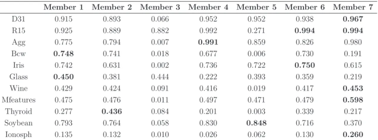
4.6 The average performance and the standard deviation of ten runs for each dataset measured by ARI. The average performance (Ave-P) of each ensemble method across 11 datasets, and the average consistency (Ave-C) are included. . . 82 4.7 The average performance and the standard deviation of ten runs for
each dataset measured by NMI. The average performance (Ave-P) of each ensemble method across 11 datasets, and the average consistency (Ave-C) are included. . . 85 4.8 The average performance and the standard deviation of ten runs for
each dataset measured by ARI. The average performance (Ave-P) of each ensemble method across 11 datasets, and the average consistency (Ave-C) are included. . . 85 4.9 The performance of the seventh members in the first run of the
exper-iment for each datasets measured by NMI. The bold value represents the maximum quality in each dataset. . . 86 4.10 The performance of the seventh members for each datasets measured
by ARI. The bold value represents the maximum quality in each dataset. 87
5.1 The Similarity MatrixSc, which is the result of measuring the
similar-ity between initials cluster vectors in our illustrative example (Figure 5.2) using Sc measure. − − − cells indicates that this similarity is
not calculated as they are placed in the same member. . . 104 5.2 The result of θ1 after we merge the most similar clusters, which are
←−c1 ={c1
1+c22+c32},←−c2 ={c12+c23+c31},←−c3 ={c13+c12}and←−c4 ={c33}104
5.3 The updated Similarity Matrix Sc after the first step of the merging
process is performed, which is the result of measuring the similarity between four clusters in θ1 (in Table 5.2) . . . 105
5.4 The result of Sx after we perform the second stage. . . 105
5.5 The updated membership similarity matrixSxafter identifying
candi-date clusters, eliminating non-candicandi-date cluster and assigning totally certain and certain objects. . . 106 5.6 The average performance and the standard deviation of ten runs for
each dataset measured by ARI. The average performance (Ave-P) of each ensemble method across 8 datasets, and the average consistency (Ave-C) are included. . . 109 5.7 The average performance and the standard deviation of ten runs for
each dataset measured by NMI Index. The average performance (Ave-P) of each ensemble method across 8 datasets, and the average con-sistency (Ave-C) are included. . . 109 5.8 The result of updating θ1 after we merge ←−c3 and ←−c4 by summing
5.9 The results of Sx after no more merging step is needed. . . 125
5.10 The results of assigning totally certain and certain objects to the candidate cluster. . . 125 5.11 The result of Sx after we perform the second stage. . . 126
5.12 Results of the first experiment listed in Table 5.6 updated by adding the average performance of ACE and the standard deviation of ten runs for each dataset measured by ARI Index. . . 129 5.13 Results of the first experiment listed in Table 5.7 updated by adding
the average performance of ACE and the standard deviation of ten runs for each dataset measured by NMI Index. . . 130 5.14 Second experiment results: the average performance and the standard
deviation of ten runs for each dataset measured by ARI. Includes the average performance of each ensemble method across 8 datasets. . . . 132 5.15 Second experiment results: the average performance and the standard
deviation of ten runs for each dataset measured by NMI. Including the average performance of each ensemble method across 8 datasets. . 132
6.1 Correlation coefficient between each diversity measure and ensemble result for each tested dataset. A bold values represent a rejection of the null hypotheses which is there is no correlation between the ensemble quality and the diversity measure. . . 157 6.2 The quality of ensembles using CO, ONCE, ACE, MCLA consensus
functions and the average member quality (Ave-mem) in 22 cases. Cases with bold font indicate that these are negative cases, which are case 1, 3, 5, 7, 9 ,11, 13, 15, 17, 18 ,19 , and 21. These cases are all taken from the results in section 6.1.2 for Thyroid dataset. . . 160 6.3 The results of ANOVA Tests on two datasets using four consensus
functions (CO, ONCE, ACE and MCLA), the bold value in the P-value column represents a statistical significant, which less than 0.05 176 6.4 The results of the Tukey test with Wine dataset using ACE and
MCLA consensus functions, the bold value in the P-value column represents a statistically significant difference between the two groups compared, which is less than 0.05 . . . 177
A.1 Statistical summary of the ensemble qualites and the generated mem-bers (Mem) in all tested datasets. . . 200 A.2 The p-value of the Correlation coefficient at the 95% confidence
Abbreviation Meaning
X Dataset
x Object
c Cluster
P Parttition/Member
Γ Set of ensemble members
m Number of ensemble members
n Number of object in X
k Number of clusters in X
Φ Clustering ensemble
CF Consensus function
Dis Distance function
S Similarity measure
CO Co-assoication matrix
ONCE Object-Neighbourhood Clustering Ensemble E-ONCE E-Object Neighbourhood Clustering Ensemble DSCE Dual-Similarity Clustering Ensemble
ACE Adaptive Clustering Ensemble MCLA Meta-Clustering Algorithm DICLENS Divisive Clustering Ensemble
Xf Friedman test
F Iman-Dave port test/ ANOVA test
CD Critical difference
P∗ Final clustering result of the ensemble
Pt Ground-truth partition of the dataset
NMI Normailsed Mutual Information
Cm Complete linkage method
B The average neighbourhood similarity matrix W The overall similarity matrix
Z The set of object pair common neighbourhood
Sc Cluster similarity
Sx Membership similarity
α1 Merging threshold
α2 Certainty threshold
θ1 Membership matrix of the newly formed clusters
λ Number of clusters inθ1
←−
C The set of all the newly formed clusters in θ1
V ar Variance
pcg Cluster certainty
DV Diversity Measure
p Pairwise Diversity Measure np Non-pairwise Diversity Measure
EOD Ensemble Output Dependent diversity measure EOI Ensemble Output Independent diversity measure cc Correlation coefficient
H Highest quality
L Lowest quality
DV+ The positive effect of diversity
DV− The negative effect of diversity
Q(Γ) Average member quality
Introduction
1.1
Background
In the context of machine learning, an ensemble is generally defined as “a machine learning system that is constructed with a set of individual models working in paral-lel, whose outputs are combined with a decision fusion strategy to produce a single answer for a given problem” [106].
The ensemble method was first introduced and well-studied in the supervised learning field. Due to its successful application in classification tasks over the past decades, researchers have attempted to apply the same paradigm to the unsupervised learning field, particularly to clustering problems. However, this may be challenging for the following two obvious reasons. Firstly, in unsupervised learning, as there is normally no prior knowledge about the underlying structure or about any particular properties that we want to find or what we consider as good solutions about the data [55, 95], different clustering algorithms often produce different clustering results for the same data. Secondly, according to the “no free lunch” theorem [108], there is no single clustering algorithm that performs consistently well in finding the correct underlying structure for different data, and there are no clear guidelines in the literature for choosing individual clustering algorithms for a given problem.
Conceptually speaking, a clustering ensemble, which is also referred to as consen-sus ensemble or clustering aggregation, can be simply defined in the same manner as for classification. In other words, it is the process of combining multiple clustering models (partitions) into a single consolidated partition [94]. In principle, an effective clustering ensemble should be able to produce better results than that of the indi-vidual clustering algorithms in terms of quality and consistency. From the clustering point of view, the quality is measured either using external information (class label) or internal information. If the external information is available the quality is defined by some degree of similarity between the clustering results and the known labels of the data (class label). If not, the quality is defined as how well the clustering result fits the data using only internal information [95]. The consistency is defined as the ability that the clustering ensemble method has to produce similar performances on a multiple number of test datasets [32].
However, the transmission from supervised learning to unsupervised learning is not as straightforward as this conceptual definition because there are some unique and challenging issues when building an ensemble for clustering. Of these issues, the key and tricky one is how to combine the clusters that are generated by the indi-vidual clustering models (members) in an ensemble, as this cannot be done through simple voting or averaging as in classification. Instead, it requires more complicated aggregating strategies and mechanisms. Therefore, developing an effective aggre-gation strategy as well as efficient is essential for building a successful clustering ensemble.
1.2
Research Motivation
This thesis focuses on two central points, which are the consensus function and the diversity of the clustering ensemble. This section explains the motivation behind them.
1.2.1
Consensus Function
A consensus function is the main component of a clustering ensemble method. It combines a number of members to produce single improved clustering results, com-pared to the individual member in the ensemble. In the past decade, a number of researchers have studied clustering ensemble methods [94, 26, 97, 27, 98].
One simple, popular consensus approach focuses on combining members by map-ping them onto a new representation, that contains similarity information. This similarity information can be estimated from members at object level or at cluster level. Generally, solving the problem of clustering the data through similarity infor-mation is not a new concept; it is a widely used concept in clustering analysis, and it is in fact the core of some of the most popular cluster algorithms such as k-means
and the hierarchical clustering algorithm. It is simple and easy to understand and implement.
In the similarity-based consensus function approach, which calculates the object pairwise similarity matrix from members, the Co-association matrix (CO) [32] is the most popular method in this approach. The idea of CO is to avoid the label correspondence problem in which the clustering result is obtained through a voting process among the objects. It assumes that similar objects are very likely clustered together by some clustering algorithm, so any objects that co-occur frequently in the same cluster should be regarded as being very similar. Each entry in CO matrix counts the number of times that a given pair of objects is placed in the same cluster among ensemble members.
However, there is a common and tricky issue that appears when roughly half of the members place some object pairs in the same cluster but the other half place them in a different cluster. In this case, we have uncertain agreement between members on how to cluster these pairs and we call them uncertain pairs of objects, and they cause problems in generating reliable consensus clustering results [111, 81]. Recently, researchers such as Wang et al. [107] and Vega-Pons et al. [103] enhanced the CO matrix to extract more information from the members. We believe that
when we build a clustering ensemble, there may be some other useful information in the generated members that could be extracted, rather than relying solely on the pairwise relationship between objects. Consequently, we were motivated to design a consensus function based on object pairwise similarity that considers more information than the pair itself to overcome the problem of the uncertain agreement to some extent.
Moreover, one obvious drawback in most similarity-based consensus functions is that they require an ordinary clustering algorithm to be applied over the similarity matrix. This leads to two adverse effects. Firstly, it is difficult to decide which one is to be used, as most of them require a parameter, so there is the question of which is the best value. Therefore, this approach unintentionally suffers from the same difficulties as the single clustering algorithm which the clustering ensemble method aims to solve. Secondly, it takes time to do a further clustering, and this makes the whole clustering ensemble inefficient.
1.2.2
Clustering Ensemble Diversity
Furthermore, it is widely believed that having diverse members in an ensemble is essential for its success. Although many researchers have investigated the effect of diversity on the quality of clustering ensembles, they have not yet arrived at any agreement on the relationship between diversity and ensemble quality. Some researchers have concluded that, through high levels of diversity among members, high levels of ensemble quality can be achieved [25, 20, 51]. By contrast, other researchers suggest that median diversity among members is better in terms of improving the ensemble’s quality [39].
Nevertheless, most of these diversity studies either investigated the effect of di-versity on one specific consensus function or their own proposed consensus function. Therefore, more studies need to be conducted in order to investigate diversity defi-nitions in their relation with multiple consensus functions.
1.3
Research Questions
The main research question that we would like to answer in this thesis is:
How can we develop an effective clustering ensemble that can improve the quality and consistency of the clustering result ? In order to answer this question, we believe this research has to consider two essential issues: consensus function and diversity by addressing the following associated questions.
1. How can we design a consensus function that addresses the problem of uncer-tain pairs of objects?
2. Is there any other information in the ensemble members that we can use to design a new effective consensus function? If so, what is it and how can we design consensus functions?
3. How can we design a similarity-based consensus approach that does not require an additional step of using an ordinary clustering algorithm to produce the final clustering result, which can be implemented in the clustering ensemble framework to generate a reliable and accurate clustering result?
4. How are the existing diversity measures defined in the context of the clustering ensemble?
5. Does the diversity influence ensemble performance?
Questions 1 to 3 are our key questions regarding to the consensus function issue, while, questions 4 and 5 are our key questions regarding to the diversity issue.
1.4
Thesis Organisation
The reminder of this thesis is organised as follows:
Chapter 2: Literature Review This chapter provides a review of clustering analysis, which includes the different clustering techniques and clustering validation
index. The clustering ensemble is then introduced in more detail. Work relating to the consensus function is discussed. Finally, this chapter details some of the current clustering ensemble applications.
Chapter 3: Research Methodology In this chapter, our research design is explained, including the adapted clustering ensemble framework, and the strategy used to test the proposed consensus functions. We also describe the implementation and tools used in our research.
Chapter 4: Object-Neighbourhood Clustering Ensemble (ONCE) In this chapter, we present two new consensus functions ONCE and E-ONCE, and discuss the results of testing the effectiveness of ONCE and E-ONCE. We also compare the performance of the proposed methods with a number of clustering ensemble methods. This chapter presents an answer to research question 1.
Chapter 5: Adaptive Clustering Ensemble (ACE) In this chapter, we de-scribe two new consensus functions based on two novel similarity measurements, which are Dual-Similarity Clustering Ensemble (DSCE) and Adaptive Clustering Ensemble (ACE). We conduct some experimental studies to test the effectiveness of DSCE and ACE and compare them to other clustering ensemble methods. We also discuss and analyse the results obtained. This chapter presents answers to research questions 2 and 3 of this thesis.
Chapter 6: The Diversity of the Clustering Ensemble In this chapter, we investigate diversity measurements by looking at their influence on ensemble performance. We analyse and discuss the experimental results obtained. Moreover, we design two experiments to investigate two issues raised from our experimental study, and discuss and analyse the results obtained. This chapter presents answers to research questions 4 and 5.
Chapter 7: Conclusions and Further Work In this chapter, we draw our overall conclusions on the two central points of this research, and we also suggest further work to be done in the future.
Literature Review
This chapter reviews the literature related to this research, including the background of clustering analysis in Section 2.1, and clustering ensembles in Section 2.2, along with details on their process. In Section 2.4, clustering ensemble applications are reviewed, and finally Section 2.5 includes a summary of this chapter.
2.1
Clustering Methods
Clustering is a task of assigning each object (sometimes called a pattern, observation or data point) in a dataset to a group or cluster in order to identify natural groups within that dataset. Thus, objects in the same cluster are more similar to each other than to the objects in the other clusters [54].
In machine learning, clustering is used to search for groups that reflect hidden structured patterns. This is widely known as unsupervised learning, in contrast to supervised learning, which requires the dataset to be labelled in advance for training purposes. The supervised learning problem is related to predicting categorical and numerical data (i.e., the data classification problem corresponds to categorical data, and the regression problem corresponds to numerical data). However, all of the available data in data clustering problems are unlabelled, so the task is to group
the objects based only on the natural relationships among them and the underlying population model [55].
The main problem in clustering is how to define any similarity/dissimilarity be-tween the objects. Generally, similarity bebe-tween two objects measures the degree to which they are alike on a numerical scale, while the dissimilarity measures the degree to which they are different
A common and important measure is the distance (Dis) between two objects. Several similarity and distance measures exist in the literature; each of them is defined based on the type of measured feature, and more details of these measures can be found in [109]. However, the best-known distance measure is the Euclidean distance. Suppose we have the datasetX ={x1, x2,· · · , xn} ∈ ℜd, where each object
xi is a set of d features (sometimes called attributes, dimensions or variables). The
Euclidean distance (E) can be calculated between two objects xi and xj as follows:
E(xi, xj) = d X l=1 |xil−xj l|2 !1/2 (2.1)
In fact, the Euclidean distance is a special case, p = 2, of the Minkowski distance (M), which is defined as follows:
M(xi, xj) = d X l=1 |xil−xj l|p !1/p (2.2)
Many techniques have been proposed for cluster analysis due to the fact that clus-tering analysis has been used in a wide variety of applications. However, we may distinguish three main types of clustering techniques: hierarchical, partitional and fuzzy. The main difference between them is that hierarchical and partitional clus-tering are classified as hard clusclus-tering, where each object in the dataset belongs to only one cluster, whereas in fuzzy clustering, which is sometimes called soft clus-tering, some objects in the dataset can belong to more than one cluster (this kind of clustering is also called overlap clustering). The following sections explain these
clustering techniques in more detail.
2.1.1
Hierarchical Clustering
Hierarchical clustering builds clusters in a hierarchy that represents the similarity levels at which the clusters are formed [57]. Compared with partitional clustering, hierarchical clustering is a nested sequence of partitions that are represented as a dendrogram (tree). Hierarchical clustering builds clusters gradually, while parti-tional clustering is a single partition that learns clusters directly [95].
Hierarchical clustering can be categorised into two different procedures: agglom-erative (bottom-up technique) and divisive (top-down technique). The agglomera-tive technique starts by assigning each object to its own cluster and then gradually merges similar clusters to form larger clusters. This continues until a stopping cri-terion is achieved. On the other hand, the divisive procedure starts by assigning all objects into one cluster and then splitting this into smaller clusters. This continues until a stopping criterion is achieved [95].
The merge or split procedure is based on the similarity between objects in a cluster and on the dissimilarity between objects in different clusters. An important example of measuring (dis)similarity between two objects is the measure of the distance between them; such measuring is called a linkage metric. There are different linkage methods, such as Single linkage, Complete linkage, Average linkage and Centroid linkage. In the Single linkage method, the distance between two clusters is defined as the minimum distance between a pair of objects drawn from the two clusters (i.e., one object from one cluster, the other from another). This is also called the nearest neighbour method. In contrast, the distance between two clusters in the Complete linkage algorithm is the maximum of all pairwise distances. In the Centroid linkage method, the distances between clusters are determined by the Euclidean distance between centroid objects. The Average linkage method considers the average pairwise distance between all objects in two clusters [95].
Although hierarchical clustering does not require information about the number of clusters, it has many disadvantages. The main disadvantage is high computational complexity, which in most algorithms is O(n3), where n is the number of objects in
the dataset. Thus, they have limited application in large datasets because a distance matrix must be calculated at each step. Moreover, it is sensitive to noise and outliers [109].
2.1.2
Partition Clustering
Partition clustering is “simply a division of the data objects into non-overlapping subsets (clusters)” [95]. It does not have a hierarchical structure, and the partition-ing is based on a specific criterion, called the criterion function, such as minimispartition-ing the sum of the squared distances. It is divided into two main sub-categories: centroid algorithms and medoid algorithms:
Centroid Algorithms These represent each cluster by centre of gravity of the objects. The best-known centroid algorithm is k-means [44], which requires the number of clusters k for the dataset to be specified, and then it partitions the data into k clusters. Cluster similarity is measured based on the mean value of the objects in the cluster, which is viewed as the cluster’s centre. Thus, all objects in the dataset are assigned to their closest centre [95]. The k-means algorithm is the best-known squared error-based clustering algorithm, which is presented below:
1. Set the value of k.
2. Select k random objects as initial centroids, Cj, j ={1, . . . , k}
3. For each object xi in dataset X.
(a) Compute the distance betweenxiand each centroidCj (for example using
the Euclidean distance as in equation 2.1) (b) Assign xi to its nearest centroid.
4. Update the centroid for each cluster by taking the mean of all the objects in that cluster.
5. Repeat steps 3 and 4 until a stable clustering result is reached and/or no change is made to the centroids.
Generally, the main property of thek-means algorithm is that it is efficient for large datasets, and it often terminates at a local optimum; the resultant clusters have spherical shapes [109]. However, it is sensitive to noise, as well as outliers in data and initial centroids, and also needs a pre-selected value fork. Each run of k-means
may generate a different clustering result [95].
Medoid Algorithms In this method, each cluster is represented by one of its elements. The best-known is the k-medoids algorithm, also called Partitioning Around Medoids (PAM) [59]. One of its advantages is that it deals with noisy data by setting the mean of a cluster to be the object that is nearest to the ‘centre’ of the cluster. Moreover, it is efficient for categorical data [109]. The key steps of
k-medoids are as follows [59]:
1. Randomly select k objects as medoids from dataset X.
2. Assign each object to its closest medoid based on the distance metric. 3. Calculate the sum of distances from all objects to their medoids.
4. Calculate a swapping cost for each pair of non-medoids and medoids. Swapping means using a non-medoid to replace a medoid. If the replacement can decrease the value of the objective function, the swap will be confirmed; otherwise, the medoid will not be replaced by the non-medoid.
5. Repeat steps 2, 3 and 4 until there is no change in the medoids.
One of the disadvantages of this method is that it assumes that each cluster can be well-represented by its medoid, which might not be the case in some datasets where this assumption cannot be applied. Moreover, because the time complexity
2.1.3
Fuzzy Clustering
This allows for an overlap between clusters; it is thus sometimes called soft clustering [109]. The best-known fuzzy clustering algorithm is c-means, which was developed by Dunn [22] and improved by Bezdek [8]. c-means assigns a degree for each object to express, if it belongs to a cluster. It is similar to k-means in that it minimises the objective function. The key steps in c-means are as follows [8]:
1. Choose a value for k clusters.
2. Randomly assign fuzzy coefficients to each object in the clusters. 3. Based on the fuzzy coefficients, compute the centroid for each cluster. 4. Based on the new cluster centres, re-calculate the coefficients of each object. 5. Compare the variance with a predefined sensitivity threshold.
6. Repeat steps 3, 4 and 5 until the variance of the fuzzy coefficients is less than the sensitivity threshold.
c-means is also sensitive to noise and outliers, and like most clustering algorithms, it requires prior knowledge of the number of clusters [109].
2.1.4
Issues with Clustering Algorithms
There are a number of issues related to clustering algorithms. Firstly, several optimal solutions are possible. Different structures for the same dataset can be achieved by a single algorithm (but with different parameters) or by several algorithms. The use of different distance metrics produces different clustering results. This makes the selec-tion of the most appropriate clusters more difficult because the data are unlabelled and the parameters cannot be tuned by using cross-validation [2]. Furthermore, exploring all possible solutions is an expensive computation and, in practice, it is infeasible for large datasets.
Secondly, the correct number of clusters for any given data is often unknown. Current applications involve increasingly complex and large datasets, which may
have complex clustering shapes, highly unbalanced clustering sizes, differing densi-ties, and possible overlap clustering; all these issues create several challenges in the selection of a suitable single clustering algorithm for extracting meaningful cluster structures [4]. Therefore, it is logical to combine multiple clustering models to build a clustering ensemble.
2.2
Clustering Ensemble Methods
Ensemble clustering is the process of combining the multiple clustering results of a set of objects into a single improved clustering. It is sometimes referred to as the Consensus solution or Clustering Aggregation. In recent years, various studies have been conducted to develop clustering ensemble methods inspired by the success of the ensemble method in the supervised learning field [94, 26, 97, 27, 98]. However, compared to the research on classification ensemble methods, building a clustering ensemble is not straightforward, and further work is required in this field.
There are several reasons that make the task of building a clustering ensemble more challenging than that of classification. One is that clustering is unsupervised learning in which the data are unlabelled, so there is no prior knowledge with which the algorithm can discover the true cluster structure, and there is no “ground truth” to validate the clustering result. Moreover, no cross-validation technique can be car-ried out to tune the clustering algorithm’s parameters, thus there are no guidelines with which the user can select the most appropriate clustering algorithm for a given dataset. Another challenge is that the number of clusters produced may differ among the generated solutions by different clustering algorithms. In addition, the number of clusters in the final solution is unknown in advance. The final solution is ob-tained by accessing a set of base solutions, which in fact are cluster labels, and not the original data used.
us-classification ensemble, where the main motivation of the latter is to improve the classification accuracy. These reasons include:
• To improve the quality of the clustering results compared to those produced by single clustering algorithms.
• To reuse existing clustering (knowledge reuse): in some applications a variety of partitions may exist, so they can be combined to obtain a final clustering result. This delivers a more consolidated clustering result; several examples are provided in [94].
• To generate robust clustering results across different types of datasets. It is widely known that the popular clustering algorithms often fail to produce a good clustering result when the data do not match with their assumptions.
Among these objectives, the first point is the most widely accepted one. The cluster quality is usually measured with a numerical measurement to assess different aspects of cluster validation [95]. Section 2.2.4 reviews some of these in more detail.
2.2.1
The Process of the Clustering Ensemble Method
Recently, Vega-Pons and Ruiz-Shulcloper [102] summarised the process of clustering ensemble into two main steps: generation and consensus. Figure 2.1 illustrates this process, in which the input is the original dataset and the output is the consensus clustering.
Generation Step This is the first step in the clustering ensemble process, where a number of ensemble members are generated by using particular generation tech-niques. Vega-Pons and Ruiz-Shulcloper [102] pointed out that greater variance in the set of ensemble members means that more information is available to the consen-sus function. Moreover, there are no constraints on how the ensemble members must be obtained [102]. Therefore, different strategies could be applied. In the literature,
Figure 2.1: The Clustering Ensemble Process [102]
several generation techniques have been used to generate members for building an ensemble; more details on these techniques can be found in section 2.2.2.
Consensus Step The second step is where the generated members are combined using a consensus function to obtain the final clustering result. The success of a clustering ensemble relies on choosing a consensus function that can improve the quality of the final clustering solution [36]. As a result, a number of consensus func-tions have been proposed in the literature; section 2.2.3 will review some common consensus functions.
2.2.2
Ensemble Generation Techniques
Some researchers have applied techniques based on the types of data or applications that have been used. For high dimensional data, Strehl and Ghosh [94] applied ran-dom feature subspaces; members are generated for each of the data subspaces. They also generated members by selecting different subsets of objects for each member. They called this technique object distribution and they applied it to big data. Fern and Brodley [25] generated members based on random projections of objects onto different subspaces, and the Expectation Maximization algorithm (EM) is applied to these subspaces. The resampling method was used by [74, 76, 5], in particular bootstrap, which is a sampling with replacement. Minaei-Bidgoli et al. [74] used
[76] used the bootstrap technique with different clustering algorithms, including k-means, model-based Bayesian clustering and self-organising map. Moreover, Ayad and Kamel [5] used bootstrap resampling in conjunction with k-means to generate the ensemble members.
Others used the most popular clustering algorithmk-means to generate the mem-bers (with a random initialisation of cluster centres). k-means has been widely used due to its simplicity and its low computational complexity [31, 97, 32, 35, 6, 51]. For instance, Fred and Jain [32] used it with random initialisations of cluster cen-tres and a randomly chosen k (number of clusters) from a pre-specified interval for each member. They used a large k value in order to obtain a complex structure within the ensemble members. They also ran k-means with a fixed k to compare the two generation techniques and they found that members with a random k are more robust than other members. Dimitriadou et al. [19] and Sevillano et al. [89] applied fuzzy clustering algorithms in particular c-means in order to generate soft clustering members, while in Hore et al. [45] they applied fuzzyk-means.
Strehl and Ghosh [94] used a graph-clustering algorithm with different distance functions for each member. Topchy et al. [98] used a weak clustering algorithm, which produces a clustering result that is slightly better than a random result in terms of quality by using two different techniques. In the first technique, they used a random projection on one dimension from the original features, whereas in the second technique they split the data into a random number of hyperplanes. The weak algorithm is simple, fast at generating members, and it has been shown that it is able to produce high-quality ensemble results.
Iam-on et al. [50] examined different techniques, including a multiple run of k-means with a fixed k for each member and a randomly chosen k from an interval, where the maximumkis equal to√n. However, settingk equal to this value appears to be unrealistic for a big dataset. Furthermore, Iam-on et al. [48] applied different generation techniques to categorical data; they rank-mode algorithm with full space and random subspaces with also a fixedkand randomk. They found that these two
techniques allowed their ensemble method to achieve high performance compared to the k-mode clustering algorithm, as well as some other ensemble methods such as those proposed by Strehl and Ghosh [94].
Another popular technique is to use different clustering algorithms for each mem-ber [111, 35], where all of the algorithms may complement each other. Yi et al. [111] used the best-known clustering algorithms, such as Hierarchical clustering and k-means. Gionis et al. [35] used the Single, Average, Ward and Complete linkage methods and k-means to generate ensemble members. Recently, Yu et al. [113] ap-plied the Gaussian mixture model in conjunction with bagging techniques. k-means
and EM were used to estimate the Gaussian mixture models’ parameters.
Iam-on et al. [48] classify the techniques used in the generation step into five categories as shown in Figure 2.2, these are:
• Homogeneous ensemble: A single clustering algorithm is used to generate a number of members.
• Different-k: Each member is generated with different randomly selected k. • Data subspace/subsample: Each member is generated by a random
sub-sample of the data, or onto different subspaces, or by using a random subset of features.
• Heterogeneous ensemble: Each member is generated using a different clus-tering algorithm.
• Mixed heuristics: Any combination of the above techniques can be mixed to generate a number of members.
2.2.3
Review of Consensus Functions
Figure 2.2: Diagram of the five categories of the ensemble generation techniques, as classified by Iam-on et al. [48].
applying well-known mathematical concepts to the problem. As the clustering en-semble is motivated by the preceding work on classification enen-sembles [64], the voting combination strategy was one of the early developments, where the labelling corre-spondence problem needs to be solved first. Another representation of the cluster labels is as categorical data [98], where some researchers represent the members as categorical features in which a category-based clustering algorithm is applied. Oth-ers transform the membOth-ers into a binary membOth-ership matrix in which the pairwise similarity matrix can be calculated [32] (i.e Co-association matrix (CO)). Other re-searchers used such a matrix to formulate a graph to which a graph-based clustering method is applied [94].
Recent reviews on clustering ensemble methods can be found in [102, 34], where the authors have been trying to classify these methods according to their techniques. Among them we consider the classification scheme originally proposed by Vega-Pons and Ruiz-Shulcloper [102] due to its simplicity. This facilitates the introduction of the main ensemble methods presented in the literature. Thus, according to them, the consensus function can be classified into two main approaches: Object Co-occurrence-based approaches and Median Partition, which are as follows:
1. The Object Co-occurrence Approach: This first computes the co-occurrence of objects in the members and then determines their cluster labels to produce a con-sensus result. Basically, it counts the occurrence of an object in one cluster, or the occurrence of a pair of objects in the same cluster, and generates the final clustering
result by a voting process among the objects. Examples of such approach are: the Relabelling and Voting method [21, 6, 114], the Co-association matrix [32] and the Graph-based method [94, 26].
2. The Median Partition Approach: This treats the consensus function as the optimisation problem of finding the median partition with respect to the cluster ensemble. The median partition is defined as “the partition that maximises the similarity with all partitions in the clustering ensemble ” [102]. Examples of this approach include the Non-Negative Matrix Factorisation based method [67], the Genetic-based method [112, 70] and the Kernel-based method [101]. More details on these methods can be found in [102].
Vega-Pons and Ruiz-Shulcloper [102] pointed out that consensus functions were primarily studied on a theoretical basis, and as a result many consensus functions based on the median partition approach were proposed in the literature, whereas only a few studies focused on the object co-occurrence approach. The following sub sections review the most common clustering ensemble methods.
2.2.3.1 Graph-based Methods
One of the early methods was proposed by Strehl and Ghosh [94], where they trans-formed the clustering ensemble problem into a graph problem, and proposed three different consensus functions: the cluster-based similarity partitioning algorithm (CSPA), the hypergraph partitioning algorithm (HGPA) and the meta-clustering algorithm (MCLA). In CSPA, the similarity matrix is used as the adjusted simi-larity matrix of a fully connected graph, where nodes correspond to objects and edge weights to their similarities. The final result is obtained by using the METIS package1 in particular PMETIS [58]. This method is similar to the evidence
accu-mulation method described by Fred and Jain [32], where the hierarchal clustering algorithm is applied to obtain the final clustering result.
On the other hand, a hypergraph is constructed in HGPA and MCLA, in which each ensemble member is represented as a hyper-edge. In HGPA, the hyper-graph is directly partitioned by cutting a minimal possible number of hyper-edges, where all hyper-edges have the same weight, into k connected nodes of approximately the same size. To do that, the authors used the hypergraph partitioning algorithm HMETIS [58]. In contrast, MCLA first defines the similarity between two clusters in terms of the amount of objects grouped in both, using the Jaccard index. Then a meta-graph is constructed where nodes represent clusters and the edges represent the similarity relations between pairs of clusters. The final partition, which is called meta-clustering, is obtained using PMETIS [58], where the meta-graph is then par-titioned intokbalanced meta-clusters. The complexity of CSPA, HGPA and MCLA is estimated in [94] as O(kn2m), O(knm), and O(k2nm2), respectively.
Furthermore, Fern et al. [26] proposed the hybrid bipartite graph formulation (HBGF) algorithm by building a bipartite graph. In this type of graph there are only two different types of nodes, and edges exist between nodes of different types. In HBGF, one type of node represents an object, whereas the other type represents clusters, and an edge exists only between the cluster and the object belonging to that cluster. Then, they applied a spectral clustering algorithm to obtain the final partition. Its computational and storage complexity is O(knm), as estimated by Fern et al. [26].
Al-Razgan and Domeniconi [2] proposed two graph-based algorithms: the weighted bipartite partition algorithm (WBPA) and the weighted subspace bipartite parti-tion algorithm (WSBPA). They combine members generated by the local adaptive clustering algorithm (LAC), which designed to work with numerical data and as-signs weights to the features in the cluster. PMETIS is also used to obtain the final clustering result. The only difference between these two algorithms is that WSBPA adds a weight vector to each cluster in the final clustering result.
2.2.3.2 Object Pairwise Similarity-based Methods
The most popular pairwise similarity-based method is the Co-association method, which avoids the labelling correspondence problem by mapping the ensemble mem-bers onto a new representation in which the similarity matrix is calculated between a pair of objects in terms of how many times a particular pair is clustered together for all ensemble members [32]. The final partition is obtained by applying any similarity-based clustering algorithm to this matrix. This method is Evidence Ac-cumulation (EAC), and each entry in the matrix represents evidence collected from all ensemble members for a pair of objects. EAC calculates the percentage of mem-bers in the ensemble in which a given pair of objects is placed in the same cluster as follows: CO(xi, xj) = 1 M M X m=1 δ(Pm(xi), Pm(xj)) (2.3)
Where xi and xj are objects, Pm is a partition, andδ(Pm(xi), Pm(xj)) is defined as:
δ=
1, if xi and xj are in the same cluster in member m.
0, if xi and xj are in different clusters in member m.
(2.4)
In Fred and Jain [32], the final partition is obtained by applying Single and Av-erage linkage hierarchical clustering algorithms to the Co-association matrix. Build-ing the hierarchical tree is achieved usBuild-ing the SBuild-ingle linkage edges with a minimum weight, which are cut based on a specific threshold. This threshold is obtained based on the decision of the number of clusters, and they defined this criterion as the range of threshold values needed to obtaink clusters, which they call the k-cluster lifetime. On the other hand, Fred [30] used a fixed threshold equal to 0.5 to obtain the final partition, where objects are joined in the same cluster if they have a similarity value greater than 0.5.
information available in the clustering ensemble, it should be noted that the original Co-association matrix [32] captures only the pairwise relationship between objects in the ensemble members. Recently (in 2009), researchers have realised that more information within the generated members can be obtained to create this matrix. Wang et al. [107] proposed Probability Accumulation (PA) which extends the Co-association method by considering the cluster size and the dimensions of the objects within the data when calculating the Co-association matrix.
In PA, a more informative similarity matrix is obtained from the ensemble mem-bers compared with the Co-association method, which means that the chance of obtaining several pairs of objects with the same similarity score is less than that of using Co-association. Vega-Pons et al. [103] proposed a weighted-association matrix that takes three different factors into consideration. These are: the number of ele-ments in the cluster to which a pair of objects belongs; the number of clusters in the ensemble member analysed; and the similarity value between the objects that were obtained by this member. They follow the same philosophy of Co-association by cal-culating the similarity matrix and then applying a hierarchical clustering algorithm and selecting the one with the highest lifetime criterion. They call this method Weighted Evidence Accumulation (WEA). In their work, they also proposed an-other algorithm based on the weighted-association matrix, by introducing a new intermediate step, called Information Unification, after the matrix is obtained. This aims to unify the different data representations and (dis)similarity measures into a new data representation, where each object is represented by (dis)similarity values (as new features).
However, we believe that there is more information in the generated members that we should consider when we calculate the similarity matrix, rather than just considering the pairwise relationship between objects.
Recently (in 2012), Yi et al. [111] highlighted an issue that is often overlooked by other methods: how to handle the uncertain data pairs when calculating the simi-larity matrix. They defined uncertain pairs of objects as the “pairs that have been
assigned to the same cluster by approximately half of the partitions in the ensemble, and assigned to different clusters by the other half” [111]. They assumed that if the number of uncertain pairs is large, then this could mislead the consensus function into producing inappropriate final result. They addressed this issue by proposing a new clustering ensemble, based on the matrix completion theory, where they filtered out the uncertain pairs in the Co-association matrix, and then they estimated their value to complete the matrix by applying a matrix completion algorithm, namely the Augmented Lagrangian as proposed by Lin et al. [68]. However, by using a matrix completion process, their approach has the disadvantage that it may cause information loss.
Moreover, a method called weighted-object clustering ensemble (WOEC) was proposed by Ren et al. [81]. It uses the Co-association matrix to define a one-shot weight assignment to objects, where a large object’s weight means that it is hard to cluster, whereas a small weight means that it is easy to cluster. In fact, they follow the same idea as the Boosting algorithm [85]. Ren et al. [81] proposed three weighted object versions of the classical clustering ensemble algorithms CSPA, HGPA and MCLA [94] reviewed earlier.
2.2.3.3 Voting-based Methods
In this kind of method, the labelling correspondence problem is first solved, and then a voting process ensues, in which each object should vote for the cluster to which it will belong in the final clustering result. Dudoit and Fridly [21] proposed a consensus function similar to the (Bagging) plurality voting used in classification ensembles, in which they solved the labelling correspondence problem using the Hungarian method [29]. They assumed that all members have the same number of clusters, and they obtained the final clustering result, which also has the same number of cluster as the members, by applying the plurality voting process.