June 2007, Volume 19, Issue 7. http://www.jstatsoft.org/
Compensating for Missing Data from Longitudinal
Studies Using
WinBUGS
Gretchen Carrigan University of Queensland Adrian G. Barnett University of Queensland Annette J. Dobson University of Queensland Gita Mishra University of Queensland Abstract
Missing data is a common problem in survey based research. There are many packages that compensate for missing data but few can easily compensate for missing longitudinal data. WinBUGScompensates for missing data using multiple imputation, and is able to incorporate longitudinal structure using random effects. We demonstrate the superiority of longitudinal imputation over cross-sectional imputation using WinBUGS. We use ex-ample data from the Australian Longitudinal Study on Women’s Health. We give a SAS
macro that usesWinBUGSto analyze longitudinal models with missing covariate date, and demonstrate its use in a longitudinal study of terminal cancer patients and their carers. Keywords: missing data, multiple imputation, longitudinal data, WinBUGS,SAS.
1. Introduction
Missing data is a common problem in survey-based research. Ignoring any missing data by using a complete case analysis can produce biased results. Biases occur when participants with complete data are systematically different from those with missing data. Longitudinal studies are especially susceptible to such bias, as missing data accumulates over time due to wave non-response and participant drop-out. One method of compensating for missing data is imputation. Over the past twenty years the body of literature on imputation theory and methodology has grown considerably and software has evolved accordingly. However, there has been relatively little work on imputation in a longitudinal setting.
approaches and identifies three classes: weighted estimating equations, multiple imputation, and likelihood-based formulations. Ibrahim et al. (2005) identify fully Bayesian as a fourth class.
Weighted estimating equations (WEE) weight records with complete data to compensate for similar cases with missing data. Most recently, literature has focussed on improving estimates of variance (Robins et al. 1994, 1995) as WEE, when unadjusted, underestimate the true variance in the data. Implementation of WEE currently relies on model-specific, user-defined algorithms, rather than standard procedures in mainstream statistical packages. Multiple imputation (MI) uses Bayesian simulation to fill in missing data, drawing together results from repeatedly imputed datasets. SeeRubin(1987) for a comprehensive coverage of multiple imputation. Fully Bayesian (FB) models extend MI methodology by jointly simulating the distributions of variables with missing data as well as unknown parameters in a regression equation. In FB the analysis and imputation models are fully and simultaneously specified. Maximum likelihood (ML) techniques also rely on fully specified models, but differ from FB in that parameter estimates are constructed using likelihood-based approximations, rather than Bayesian simulation.
Maximum likelihood approaches to imputation are often intractable in mainstream software packages. Implementation relies upon strict assumptions about patterns of missingness that are frequently violated in complex survey data. While MI procedures exist in a range of software packages such as SAS (SAS Institute Inc. 2003), Stata (StataCorp. 2003), S-PLUS (Insightful Corp. 2003), and R (R Development Core Team 2007), they generally rely on the assumption that data are multivariate normal or can be approximated by a multivariate normal distribution (Schafer 1997). More recent work on chained regression equations has led to a number of add-on packages that can incorporate categorical data: MICE in S-PLUS(van Buuren and Oudshoorn 1999),IceinStata(Royston 2005), and IVEwareforSAS (Raghunathan et al. 2002). However, the authors have still had difficulty in incorporating longitudinal information into the imputation methodology of these programs. FB techniques are most suited to longitudinal imputation, as they can incorporate hierarchical structure into the modelling process, and, like chained regressions, they have the capability to systematically deal with categorical data. The software packages WinBUGS (Spiegelhalter et al. 2003) and
MLwiN (Rasbash et al. 2005) both use a FB framework. Cowles (2004) and Woodworth (2004) both provide a useful overview to WinBUGS, while Carpenter and Kenward (2005) and Congdon (2001) present introductory examples of FB imputation with missing data. Pettittet al.(2006) andQiuet al.(2002) present thorough analyses in the context of missing categorical data.
The aim of this paper is to demonstrate WinBUGS’s capacity to compensate for missing longitudinal data, with a particular focus on missing covariate data. We do this by looking at a longitudinal analysis of diabetes incidence in Australian women. In Section 2 we introduce the motivating example from the Australian Longitudinal Study on Women’s Health. In Section 3 we specify a fully Bayesian model for the incidence of diabetes without and with missing covariate data. In Section4we describe its implementation inWinBUGS, and present the results in Section 5. In Section6 we give a generalSAS macro (that calls WinBUGS) for analysing longitudinal models with missing covariate data. We conclude with a discussion and some recommendations in Section7.
2. Motivating example
Women who are overweight have an increased risk of developing diabetes. However the relative impact of longer-term adiposity and short-term weight changes on the incidence of diabetes is of scientific interest (Mishraet al. 2007). The Australian Longitudinal Study on Women’s Health (ALSWH) is designed to answer such questions as it tracks over time the health and well-being of a representative sample of Australian women (Lee, Dobson, Brown, Bryson, Byles, Warner-Smith, and Young 2005).
The ALSWH study collects self-reported data from mail-out surveys every two to three years. For this analysis we used data from the mid-aged cohort of women who were aged 45 to 50 at the time of the initial survey in 1996 (S1). Subsequent surveys occurred in 1998 (S2), 2001 (S3), and 2004 (S4). At S1 13,716 women agreed to take part in the longitudinal study and by S4 10,905 women remained. Key variables for the analysis of diabetes incidence and weight are outlined below.
At S1 women were asked if they had ever been diagnosed with diabetes. At S2, S3 and S4 women were asked if they had been diagnosed with diabetes since the previous survey. Using this data women were classified into one of the following groups: existing case at S1, incident case between S1 and S2, incident case between S2 and S3, incident case between S3 and S4, free from diabetes, or unknown.
Women were asked to report their height and weight at each survey. Self-reported heights from the first three surveys were used to obtain a single estimated value for each woman by averaging the available data. Body mass index (BMI) for each woman at S1 was calculated as self-reported weight (kilograms) at S1 divided by the square of estimated height (metres). BMI was categorized as (according to theWorld Health Organization(2000)): ‘underweight’,
<18.5 kg/m2; ‘healthy weight’, [18.5, 25) kg/m2; ‘overweight’, [25, 30) kg/m2; ‘obese’, [30, 35) kg/m2; or ‘very obese’,≥35 kg/m2. Fewer than 2% of women were classified as ‘underweight’
at S1, so this category was combined with the ‘healthy weight’ group.
At S1 women were asked what they would like to weigh. Responses were categorized into: happy/like to weigh more, like to weigh 0 to 5 kg less, like to weigh 5 to 10 kg less, like to weigh more than 10 kg less.
3. Model specification
Examining the association between health and weight is often difficult in survey data because weight is a sensitive question and is sometimes not reported. For example, in the ALSWH at S1 545 women (4.0%) did not report their weight, whereas for the other variables used in this paper the average percent of missing was 1.3%. If women who are overweight are less likely to report their weight then a complete case analysis could well underestimate the true association between weight and diabetes incidence.
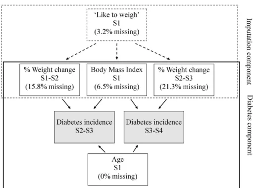
Figure1gives a graphical summary of our model. The model is split into the imputation and diabetes components. In the diabetes component we examined the association between BMI at S1 and annual percentage weight change on the incidence of diabetes, adjusting for age at baseline. BMI at S1 represented longer-term adiposity while annual percentage weight change represented short-term weight change. Because we were interested in weight change before diabetes onset, weight change was measured in the survey period prior to reported incidence
Figure 1: Model of the association between diabetes incidence and long-term BMI and short-term changes in weight
(to avoid the risk of ‘reverse causation’ whereby women who were diagnosed with diabetes subsequently lost weight). Therefore, the study population for the analysis was confined to those women who became an incident case between S2 and S3 or S3 and S4, or those who were free from diabetes. Women who became an incident case between S2 and S3 were excluded from the analysis in the following period as they were no longer in the population at risk. As shown in Figure1there were different amounts of missing covariates, with likely different reasons for why they were not completed. Rubin defines three potential patterns of miss-ingness: missing completely at random (MCAR), in which there is no systematic difference between the characteristics of those with and without missing data; missing at random (MAR), in which there is a systematic difference but this can be explained by other observed data; and missing not at random (MNAR) where the difference cannot be explained by observed data.
We relied on the MAR assumption to build an imputation component into the model using the question, “How much would you like to weigh?” There were far fewer missing responses to the ‘like to weigh’ question compared with actual weight. Also, the ‘like to weigh’ variable at S1 was highly correlated with self-reported weight at all surveys (Mishra and Dobson 2004). Hence we used ‘like to weigh’ to impute missing weights at each survey. For each imputed weight we recalculated BMI at S1 and percentage weight change. Women for whom height was unknown (3.2%) or who didn’t respond to the ‘like to weigh’ question (3.2%) were excluded from the analysis.
(i) A complete case model (7113 women),
(ii) A cross-sectional imputation model (9557 women),
(iii) A longitudinal imputation model using random effects to incorporate within-subject correlation (9557 women).
Models (ii) and (iii) both had the diabetes and imputation component (Figure 1). Model (i) only had the diabetes component.
We now describe the three models in more detail.
3.1. Complete case model
LetYit be a binary variable denoting incidence of diabetes for individual i (i= 1, . . . ,7113)
at time t(t= 1,2). The complete case model is then,
Yit ∼ Bernoulli(pit),
logit(pit) = αt+XiTβ+Zi(t−1)Ψ
where X is a matrix of the time-invariant covariates (BMI at S1, age at S1), Z is a vector containing the single time varying covariate (percentage weight change in the survey period prior to reported incidence) and α is an intercept that varies according to survey (time).
3.2. Cross-sectional imputation model
The diabetes component of this model followed the same structure as the complete case model. In the imputation component of the model, we assumed that the weight of individual i(i= 1, . . . ,9557) at surveys(s= 1, . . . ,4) was distributed as:
Wis ∼ Normal(µis, σ2),
µis = γ+ϕt+LTi φ,
whereLis a vector containing the response of each individualito the ‘like to weigh’ question. Thus weight for individual i at survey s was described by a population mean γ plus an increment of ϕat each survey, and was adjusted according to the response of individual ito ‘like to weigh’ at S1 (φ). The estimates of γ, ϕand φ were based on records with partial or complete data. Women with a missing weight (Wis) had their weight imputed from a Normal
distribution with mean ˆµis and variance ˆσ2.
Note that the diabetes component is evaluated over two time periods (t= 1,2, surveys 3 and 4) whereas the weight component is evaluated over four time periods (s= 1,2,3,4, surveys 1 to 4). This meant that we used the maximum amount of information to impute weight, whilst excluding surveys 1 and 2 from the diabetes component because we were only interested in incident cases.
3.3. Longitudinal imputation model
The diabetes component of the model followed the same structure as the complete case model. We introduced a random intercept into the imputation component of the model to incorporate
within-subject correlation in weight, and hence take account of the longitudinal study design. The imputation component for weight was:
Wis ∼ Normal(µis, σ2b),
µis = γi+ϕt+LTi φ,
γi ∼ Normal(λ, σw2).
Instead of a population mean for weight, each subject had her own estimate (γi, known as
a random intercept). The total variance in weight from the previous model (σ2) has been partitioned into the within-subject variance σw2, and the between-subject variance σb2. The within-subject correlation is given by ρ=σb2/(σb2+σw2).
3.4. Inference using Gibbs sampling
The models that we have presented above use two parametric distributions (Bernoulli and Normal), with many parameters at several hierarchical levels. An analytical solution to the model is therefore intractable. Fortunately we can make inference about the parameters using Gibbs sampling (the default method in WinBUGS). In Gibbs sampling each unknown parameter is estimated conditional on all the other observed data and the other estimated parameters (for a detailed description of Gibbs sampling see Gelman et al. (2004)). For example, in the hierarchical imputation model, a missing weight would be sampled from a normal distribution with mean ˆµis and variance ˆσ2. A complete iteration occurs when all
the parameters and missing data have been estimated. The next iteration is then based on these estimates and the data. To start the iterations an initial set of values for each unknown parameter and observation is specified. Many iterations are run (usually greater than 1000) in an attempt to converge to a solution. We discuss some of the practical issues of running such iterations in the next section.
4.
WinBUGS
code
To run an analysis inWinBUGS there are four basic requirements: specify a model; load the data; specify initial values; and run the Gibbs sampler. This process is most efficient when the above information is stored in four batch files: an input data file; a file containing the model specification; an initial values file; and a script file that executes WinBUGS commands. We focus here on the model specification file, illustrating the conversion of our three models into a WinBUGS format. Model specification in WinBUGS differs from other standard statistical packages in that the model must be fully and explicitly specified by the user, rather than inserting model specifications into pre-programmed statistical procedures. Information on the construction of the remaining batch files is in AppendixA.
4.1. Complete case model
The first lines of code are:
model{
for (i in 1:7311){
The model statement opens the model specification file. We looped through records for 7311 individuals at two time points, except where a woman first reported diagnosis of diabetes at S3, in which case she was no longer included in the population at risk at S3 and data from a single time point was used. This condition was achieved through the use of the indicator variable, nsurvey, which took the value of 1 when diabetes incidence occurred between S2 and S3, and took the value of 2 otherwise.
In this modelt= 1 refers to diabetes incidence between S2 and S3 and weight change between S1 and S2. Similarlyt= 2 refers to diabetes incidence between S3 and S4 and weight change between S2 and S3. BMI and age at S1 did not change over time.
We specified the distribution of diabetes incidence (diab) to be Bernoulli,
diab[i,t] ~ dbern(diab.prob[i,t]);
Ending statements with a semi-colon is optional inWinBUGS.
Our interest lay in the parameterdiab.prob, which represents the probability of becoming an incident case of diabetes. We modelled the relationship between the probability of diabetes and other explanatory variables as follows.
logit(diab.prob[i,t]) <- d.int + (d.time*equals(t,2)) + (d.wtspc*wtspc[i,t]) + (d.bmi[1]*equals(bmi[i],2)) + (d.bmi[2]*equals(bmi[i],3))
+ (d.bmi[3]*equals(bmi[i],4)) + (d.age*age[i]);
The equals function was used with the integer value of t (representing time) to turn the parameterd.time ‘on’ for time 2 and ‘off’ for all other times. Hence the parameter d.time
estimates the change in diabetes risk at S4 compared to S3 (all estimated parameters for the diabetes components have a ‘d.’ prefix). We also used theequalsfunction to create indicator variables for categories of BMI.
We specified non-informative priors for each of the unknown parameters in the bottom tier of the hierarchy. We did this by assigning each unknown parameter a normal distribution with a zero mean and small precision dnorm(0.0,1.0E-6), where the precision is the inverse of the variance.
4.2. Cross-sectional imputation model
The specification of the diabetes component of the model was very similar to the complete case model. As above, we modelled diabetes as a Bernoulli variable.
diab[i,t] ~ dbern(diab.prob[i,t]);
However, to assist with convergence, we imposed a constraint on the minimum value that
diab.probcould take (as very small probabilities led to non-estimable likelihoods).
diab.prob[i,t] <- max(0.0001, diab.temp[i,t]);
logit(diab.temp[i,t]) <- d.int + (d.time*equals(t,2)) + (d.wtspc*wtspc[i,t]) + (d.bmi[1]*step(1.9-bmi[i,t])) + (d.bmi[2]*step(2.9-bmi[i,t])) + (d.bmi[3]*step(3.9-bmi[i,t])) + (d.age*age[i]);
With the introduction of missing data in weight, BMI became a stochastic variable in the model. For this reason, we could not use theequalsfunction to create an indicator function for BMI. The problem was overcome by using thestepfunction, with thresholds set at some value between the integer categories. Further explanation on the use of the indicator functions
stepand equals can be found in theWinBUGS user’s manualSpiegelhalteret al. (2003). The imputation component of the model focussed exclusively on the imputation of weight at each survey, which is used to calculate both BMI and percentage weight change. Where weight for individual i at survey s was unknown, we specified the distribution of weight to be Normal. Our interest lay in the relationship between the mean value of weight and other information contained within the existing data, as shown below.
for (s in 1:4){
wtkg[i,s] <-cut(wtkg.uncut[i,s]);
wtkg.uncut[i,s] ~ dnorm(wt.mu[i,s],wt.tau);
wt.mu[i,s] <- w.int + (w.slo*s) + (w.like[1]*equals(like[i],2)) +
(w.like[2]*equals(like[i],3)) + (w.like[3]*equals(like[i],4));}
We used the cut function to prevent ‘feedback’ from the results from diabetes influencing the imputed weights. In other words to maintain the flow of information as indicated by the arrows in Figure 1.
This above code was embedded within the ‘individual’, or ‘i’, loop but external to the ‘t’ loop in which the diabetes component was contained. This enabled weight to be modelled using data from all four surveys and in so doing, ensured that the imputation model incorporated all available information. Weight was not a variable of direct interest so we used logical functions to recalculate the variablesbmi(categorical) and wtspc(continuous) as follows.
wtspc[i,t] <- ((wtkg[i,t+1]-wtkg[i,t])/wtkg[i,t])/(t+1)*100; bmic[i,t] <- wtkg[i,1]/(height[i]*height[i]);
bmi[i,t] <- 1 + step(bmic[i,t]-25) + step(bmic[i,t]-30) + step(bmic[i,t]-35);
4.3. Longitudinal imputation model
The diabetes component of the model was the same as that in the cross-sectional model. The imputation component required only a slight modification to the intercept term, and one new line of code to describe the distribution of the random intercept.
for (s in 1:4){
wtkg[i,s] <-cut(wtkg.uncut[i,s]);
wtkg.uncut[i,s] ~ dnorm(wt.mu[i,s],wt.tau);
wt.mu[i,s] <- w.int[i] + (w.slo*s) + (w.like[1]*equals(like[i],2)) + (w.like[2]*equals(like[i],3)) + (w.like[3]*equals(like[i],4));} w.int[i] ~ dnorm(w.mu,w.tau);
We compare the fit of the three models using the Deviance Information Criterion (DIC) (Spiegelhalteret al. 2002) and using 10-fold cross-validation (Breimanet al. 1984).
5. Results
Analyses for each of the three models were performed inWinBUGS, Version 1.4.1. Each model was run for 25,000 iterations, with an additional 5000 iterations for burn-in. The time taken to run the longitudinal imputation model (the most complex) inWinBUGS was 53 minutes, using a server running Microsoft Windows Server 2003 Enterprise Edition with dual 3.6 GHz Xeon processors and 6 GB of RAM. The length of time is mostly dependent upon the number of observations in the data and the number of iterations required.
To compare the results fromWinBUGSwith another package, the complete case analysis was also implemented inSAS, Version 9.1.3, usingproc genmodwith the optionstype=exch and
d=binomialandlink=logit.
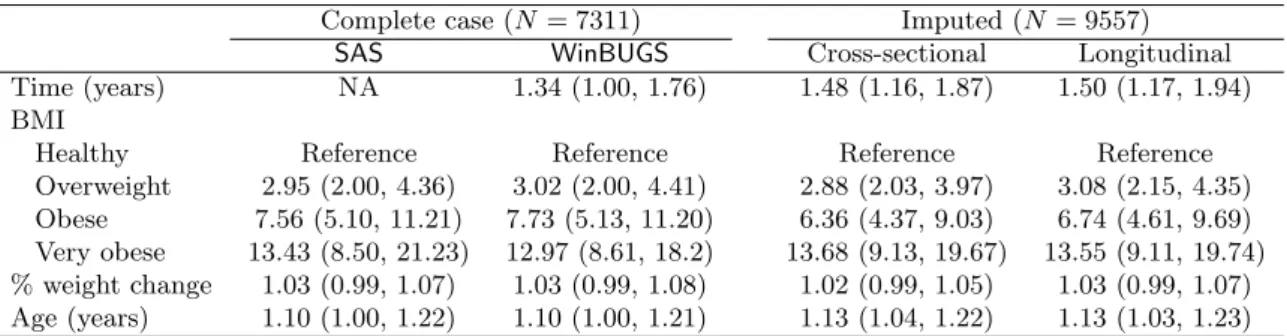
Odds ratios for incidence of diabetes in each of the three models are shown in Table1. There was little difference in the odds ratios for diabetes, or their posterior limits, between the various models and two packages. Nor did the interpretation of the results change, with the main result being that long-term obesity (BMI) was a stronger predictor of diabetes incidence compared to short-term weight gain (Mishraet al.2007).
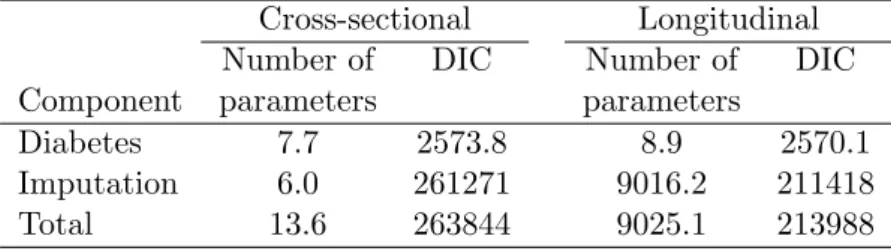
The longitudinal model was a better fit to the data than the cross-sectional model as the longitudinal model had a smaller DIC (Table 2). The longitudinal model used many more parameters as each woman had her own intercept. This large increase in parameters gave a much improved fit to the imputation component of the model. This improved imputation gave a slightly better fit to the diabetes component (DIC of 2570.1 vs 2573.8).
The results of the 10-fold validation were similar to those from the DIC. For the cross-sectional model the average error for an imputed weight was 10.4 kilograms (standard devi-ation (SD) = 0.23 kg). For the longitudinal model the average error was a much smaller 5.3 kilograms (SD = 0.17 kg). The cross-validation found little difference between the models in terms of their fit to the diabetes component. For the cross-sectional model the average area under the receiver operating characteristic (ROC) curve for predicted diabetes (yes/no) was 0.548. For the longitudinal model the average area under the ROC curve was 0.543.
6. A more general
SAS
macro
In this section we describe aSASmacro for analysing general longitudinal models with missing covariate data. The macro converts aSASdata set toWinBUGSformat and writesWinBUGS
Complete case (N= 7311) Imputed (N = 9557) SAS WinBUGS Cross-sectional Longitudinal Time (years) NA 1.34 (1.00, 1.76) 1.48 (1.16, 1.87) 1.50 (1.17, 1.94) BMI
Healthy Reference Reference Reference Reference Overweight 2.95 (2.00, 4.36) 3.02 (2.00, 4.41) 2.88 (2.03, 3.97) 3.08 (2.15, 4.35) Obese 7.56 (5.10, 11.21) 7.73 (5.13, 11.20) 6.36 (4.37, 9.03) 6.74 (4.61, 9.69) Very obese 13.43 (8.50, 21.23) 12.97 (8.61, 18.2) 13.68 (9.13, 19.67) 13.55 (9.11, 19.74) % weight change 1.03 (0.99, 1.07) 1.03 (0.99, 1.08) 1.02 (0.99, 1.05) 1.03 (0.99, 1.07) Age (years) 1.10 (1.00, 1.22) 1.10 (1.00, 1.21) 1.13 (1.04, 1.22) 1.13 (1.03, 1.23) Table 1: Odds ratios (and 95% confidence/posterior limits) for incidence of diabetes
Cross-sectional Longitudinal Number of DIC Number of DIC Component parameters parameters
Diabetes 7.7 2573.8 8.9 2570.1 Imputation 6.0 261271 9016.2 211418 Total 13.6 263844 9025.1 213988
Table 2: Comparisons of model fit for cross-sectional and longitudinal models (DIC = De-viance Information Criterion)
code to run a longitudinal model. It then reads the results fromWinBUGS and summarizes them inSAS.
This particular macro is restricted to models with a continuous dependent variable and so is more limited than the models used in section 4. Multiple covariates are allowed and these may be either categorical or continuous. However, the covariate with missing data must be continuous and time-dependent (i.e., change over time). This macro uses a simpler model than that discussed in the previous section for the diabetes data set. The model for diabetes included specific functions (such as calculating body mass index from weight) and used different time periods for the model of interest and imputation model. Such specific programming can be added to the WinBUGScode generated by ourSAS macro.
We demonstrate the SAS macro for a continuous dependent variable with a smaller longitu-dinal data set from a study of terminal cancer patients and their carers (Correa-Velezet al. 2003). The outcome is the carer’s level of anxiety, measured on the hospital anxiety and de-pression scale (HADS), for which higher scores indicate greater anxiety (Zigmond and Snaith 1983). In this study patients and their carers were regularly interviewed during the final year of life. The study was particularly interested in how patient anxiety impacted on carer anxi-ety. Both patient anxiety and carer anxiety had some missing values. The other variables are the carer’s gender, the time to death (in weeks), and the patient’s number of symptoms. The number of symptoms and anxiety scores are time-varying covariates. The data set contains 514 interviews from 109 carers.
Using the terminal cancer data ourSASmacrolongimpis called using the following statement (note the text between ‘/*’ and ‘*/’ is comment and can be omitted):
%longimp(dsetin=data.carer, /* Input data set */
depvar=hadsanx, /* Dependent variable (model of interest) */
vars=phadsanx gender deathwks, /* Explanatory var(s) (model of interest) */ class=gender, /* Class explanatory variable(s) (model of interest) */
depvari=phadsanx, /* Dependent variable (imputation model, continuous) */ varsi=count, /* Explanatory variable(s) (imputation model) */
classi=, /* Class explanatory variable(s) (imputation model) */ time=interno, /* Time variable */
repeated=carerid, /* Repeated variable (e.g. subject) */
centre=Y, /* Centre continuous explanatory variables (Y/N), default=Y */ MCMC=5000 /* Number of MCMC iterations & burn-in, default=1000 */
The dependent variable in the model of interest is the carer’s anxiety (depvar=hadsanx). This is dependent on: their gender (which is a categorical variable,class=gender), their patient’s level of anxiety (phadsanx) and the time to patient’s death (deathwks). The patient’s level of anxiety is a time-dependent covariate and has some missing values. We impute these missing values by making them the dependent variable of the imputation model (depvari=phadsanx). The patient’s level of anxiety is dependent on their number of symptoms (count). There are no missing values for the number of symptoms.
The other necessary inputs are the variable that defines time, which in this case is the inter-view number (time=interno), and an identification number for each carer which links their repeated results (repeated=carerid).
There is the option to centre the continuous explanatory variables by subtracting their mean (centre). This is generally advisable inWinBUGSas it often improves the convergence of the MCMC algorithm. The final option is to choose the number of MCMC iterations and burn-in (MCMC).
The aboveSAS macro call produces the following four pages of output:
Longitudinal model using WinBUGS 1 Model information
Input data set: work.carer Dependent variable: hadsanx Observations: 514
Subjects/Clusters: 109
Longitudinal model using WinBUGS 2 Geweke’s MCMC converge diagnostic
Mean
Variable difference df t-value p-value
count -0.00057 2998 -0.24445 0.80690 deathwks 0.00082 2998 1.47354 0.14071 gender_1 0.11865 2998 3.30014 0.00098 intercept -0.01108 2998 -0.46386 0.64278 intercept_i -0.01178 2998 -0.86887 0.38499 phadsanx 0.00506 2998 1.90966 0.05627
Longitudinal model using WinBUGS 3 Parameter estimates - Model of interest
95% Posterior Interval Variable Mean SD Lower Upper
intercept 6.464 0.486 5.556 7.479 deathwks 0.039 0.011 0.016 0.062 gender_1 -2.649 0.756 -4.112 -1.203
phadsanx 0.288 0.054 0.182 0.390 sigma2 8.377 0.610 7.278 9.656 rho 0.597 0.047 0.502 0.684
Longitudinal model using WinBUGS 4 Parameter estimates - Imputation model
95% Posterior Interval Variable Mean SD Lower Upper
intercept_i 0.263 0.271 -0.281 0.792 count 0.351 0.046 0.261 0.443
The first page of output gives some basic information on the model. The second page gives the MCMC convergence diagnostic of Geweke (1992). This compares the first 10% of the chain to the last 50%. It is important for valid inference to have MCMC chains that are stable and have converged. A chain that has converged should have a constant mean and the output compares the means of the first and last sections of the chain using an unpaired
t-test. In this case the mean for the gender variable seems to have increased slightly. The chain should be run again (possibly for longer) to give a more stable estimate for gender. The third and fourth pages give the parameter estimates from the model of interest and the imputation model. The results show that as the patient’s death approached the carer’s anxi-ety increased (deathwks). Also male carers had much lower anxiety (gender), and increased patient anxiety was associated with increased carer anxiety (phadsanx). The average anxi-ety score was 6.464 (intercept) and the variance was 8.377 (sigma2). The within-subject correlation for carers was a relatively strong 0.597 (rho), indicating a good deal of similarity over time in each carer’s anxiety level. For the imputation model the patient’s number of symptoms was positively associated with their level of anxiety (count).
7. Discussion
Survey data is often partially completed and using a complete case analysis can produce biased results. For an example used here concerning the risk of diabetes incidence this was not the case, as a complete case analysis and analyses after imputation gave similar estimates. However, the complete case analysis used data from 7311 women, whereas the analyses using imputation used data from 9557 women (a 31% increase). Using a larger sample generally gives results that are more representative.
In our example concerning diabetes incidence there was no difference between the parameter estimates from a cross-sectional imputation model and a model that exploited the longitudinal structure of the data. However, the longitudinal imputation model gave better estimates of missing weights as shown by the cross-validation (mean error of 5.3 kg for the longitudinal model compared to 10.4 kg for the cross-sectional). Hence we still strongly recommend the use of longitudinal imputation when the data structure is longitudinal.
Much of the software available for imputation is yet to develop capabilities for longitudinal imputation, and instead uses cross-sectional imputation. WinBUGS, on the other hand, can incorporate longitudinal structure with relative ease. As illustrated in Section 4, there was
little difference in the longitudinal and cross-sectional imputation code. WinBUGS is also able to easily deal with missing categorical data, whereas many other packages rely on an assumption of Normality. We have provided aSAS macro for analysing longitudinal studies with missing covariates that usesWinBUGSbut is able to be run from SAS.
References
Breiman L, Friedman J, Olshen R, Stone C (1984). Classification and Regression Trees. Wadsworth Statistics/Probability Series. Wadsworth International Group, Belmont, Cali-fornia.
Carpenter J, Kenward M (2005). “Example Analyses Using WinBUGS 1.4.” URL http: //www.missingdata.org.uk/.
Congdon P (2001). Bayesian Statistical Modelling. Wiley Series in Probability and Statistics. Wiley, Chichester; New York.
Correa-Velez I, Clavarino A, Eastwood H, Barnett A (2003). “Use of complementary and alternative medicine and quality of life: changes at the end of life.” Palliative Medicine,
17, 695–703.
Cowles MK (2004). “Review of WinBUGS1.4.”The American Statistician,58(4), 330–336.
Gelman A, Carlin JB, Stern HS, Rubin DB (2004). Bayesian Data Analysis. Texts in Statis-tical Science. Chapman & Hall/CRC, Boca Raton, Fla., 2nd edition.
Geweke J (1992). “Evaluating the accuracy of sampling-based approaches to calculating posterior moments.” In J Bernado, J Berger, A Dawid, A Smith (eds.), “Bayesian Statistics 4,” Clarendon Press, Oxford, UK.
Ibrahim JG, Chen MH, Lipsitz SR, Herring AH (2005). “Missing-data Methods for Generalized Linear Models: A Comparative Review.”Journal of the American Statistical Association,
100(469), 332–346.
Insightful Corp (2003). S-PLUS Version 6.2. Seattle, WA. URL http://www.insightful. com/.
Lee C, Dobson AJ, Brown WJ, Bryson L, Byles J, Warner-Smith P, Young AF (2005). “Cohort Profile: The Australian Longitudinal Study on Women’s Health.”International Journal of Epidemiology,34(5), 987–991.
Mishra GD, Carrigan G, Brown WJ, Barnett AG, Dobson AJ (2007). “Short-Term Weight Change And The Incidence Of Diabetes In Midlife: Results From The Australian Longitu-dinal Study Of Women’s Health.”Diabetes Care.
Mishra GD, Dobson AJ (2004). “Multiple Imputation for Body Mass Index: Lessons from the Australian Longitudinal Study on Women’s Health.”Statistics in Medicine,23, 3077–3087.
Pettitt AN, Tran TT, Haynes MA, Hay JL (2006). “A Bayesian Hierarchical Model for Categorical Longitudinal Data from a Social Survey of Immigrants.” Journal of the Royal Statistical Society A,169(1), 97–114.
Qiu Z, Song PXK, Tan M (2002). “Bayesian Hierarchical Models for Multi-level Repeated Ordinal Data Using WinBUGS.”Journal of Biopharmaceutical Statistics,12(2), 121–135.
Raghunathan TE (2004). “What do we do with Missing Data? Some Options for Analysis of Incomplete Data.”Annual Review of Public Health,25, 99–117.
Raghunathan TE, Solenberger P, Van Hoewyk J (eds.) (2002). IVEware: Imputation and Variance Estimation Software Users Guide. University of Michigan: Survey Research Cen-ter, Institute for Social Research.
Rasbash J, Steele F, Browne W, Prosser B (2005). A User’s Guide to MLwiN Version 2.0. University of Bristol, Bristol. URLhttp://www.cmm.bris.ac.uk/MLwiN/download/ manuals.shtml.
RDevelopment Core Team (2007).R: A Language and Environment for Statistical Computing. RFoundation for Statistical Computing, Vienna, Austria. ISBN 3-900051-07-0, URLhttp: //www.R-project.org/.
Robins JM, Rotnitzky A, Zhao LP (1994). “Estimation of Regression Coefficients when some Regressors are not Always Observed.” Journal of the American Statistical Association,
89(427), 846–866.
Robins JM, Rotnitzky A, Zhao LP (1995). “Analysis of Semiparametric Regression Models for Repeated Outcomes in the Presence of Missing Data.”Journal of the American Statistical Association,90(429), 106–121.
Royston P (2005). “Multiple Imputation of Missing Values: Update.” The Stata Journal,5, 1–14.
Rubin DB (1987). Multiple Imputation for Nonresponse in Surveys. J. Wiley & Sons, New York.
SAS Institute Inc (2003). SAS/STAT Software, Version 9.1. Cary, NC. URL http://www. sas.com/.
Schafer JL (1997). Analysis of Incomplete Multivariate Data. Monographs on Statistics and Applied Probability. Chapman & Hall, London.
Spiegelhalter DJ, Best NG, Carlin BP, van der Linde A (2002). “Bayesian Measures of Model Complexity and Fit (With Discussion).” Journal of the Royal Statistical Society Series B,
64, 583–640.
Spiegelhalter DJ, Thomas A, Best NG, Lunn D (2003). WinBUGSVersion 1.4 User Manual. MRC Biostatistics Unit, Cambridge. URLhttp://www.mrc-bsu.cam.ac.uk/bugs/. StataCorp (2003). StataStatistical Software: Release 8. StataCorp LP, College Station, TX.
URLhttp://www.stata.com/.
Sturtz S, Ligges U, Gelman A (2005). “R2WinBUGS: A Package for RunningWinBUGSfrom R.”Journal of Statistical Software,12(3), 1–16.
van Buuren S, Oudshoorn K (1999). “Flexible Multiple Imputation by MICE.” Tech-nical Report PG/VGZ/99.054, TNO Prevention and Health. URL http://www. multiple-imputation.com/.
Woodworth GG (2004).Biostatistics: A Bayesian Introduction. Wiley-Interscience, Hoboken, NJ.
World Health Organization (2000). “Obesity: Preventing and Managing the Global Epidemic.” Technical Report 894, WHO Technical Report Series.
Zigmond AS, Snaith RP (1983). “The Hospital Anxiety and Depression Scale.”Acta Psychi-atrica Scandinavica,67, 361–370.
A. Batch files in
WinBUGS
A.1. Input data fileRaw data are values of the variables: diabetes, weight (at each survey), age, height, like to weigh, and the indicator variable: nsurvey.
Data can be entered into WinBUGS in one of two ways: the list format of S-PLUS, or as a series of one dimensional arrays, in a tab delimited file. In both cases, the hierarchical dimensions of the data must be specified by the user. Data are stored as .txt files. Missing data is entered as ‘NA’.
WinBUGS is not suited to data management, and so for large data sets another package is required. We usedSAS, Version 9.1.3, creating our data files as tab delimited text. It is also possible to useRand the packageR2WinBUGSin the management of large data sets (Sturtz et al.2005).
Using the data array format, data was entered under the following column headings (we also show three example lines of data):
diab[,1] diab[,2] wtkg[,1] wtkg[,2] wtkg[,3] wtkg[,4] age[] height[] like[] nsurvey[]
1 NA 40.5 30.2 NA 35.5 51 140 1 1 0 1 89.8 89.6 75.5 99.2 52 160 4 2 0 0 65.2 65.4 66.7 NA 50 175 2 2 ...
The last line of a data file of this format must be the word ‘END’ and the return key must be entered forWinBUGS to read the file correctly.
A.2. Initial values file
Initial values can be specified in one of two ways: by the user, or as randomly generated values using the gen.inits() command in the WinBUGS script file. It is also possible to specify some initial values and then use thegen.inits() function to create the remainder. User specified values are stored in a .txt file whose structure follows the same protocol as the data file. It is often necessary for the user to specify ballpark initial values as gen.inits()
can generate unreasonable starting values, which in turn means thatWinBUGScannot begin to iterate the Gibbs sampler.
WinBUGStreats each unobserved record in a variable with missing data as a random variable whose distribution must be estimated. To specify the initial values for these unobserved records we must enter a matrix of values that matches the dimensions of the variable. If a record is observed, then the entry in the initial value matrix is ‘NA’, otherwise, if the record is unobserved, the entry is the user-specified initial value.
A.3. Script file
The script file is a list ofWinBUGScommands which are executed sequentially and activated by the ‘Script’ option in the Model menu. The following commands must be included in this file, in the sequence shown below, for the model to run.
check(’path/filename’): Calls the model specification file and scans for errors in syntax. Notice the forward slash in the file path.
load(’path/filename’): Calls the data file.
compile(n): Ensures that the model specification file and the data file are compatible. n
denotes the number of chains to run simultaneously.
inits(n,’path/filename’): Calls the initial values file/s.
gen.inits(): Generates initial values not specified in the initial values file. Not necessary if initial values have already been fully specified by the user.
update(n): Begins the MCMC simulation and runs forniterations
Additional commands are required to view the output. Set(name) indicates that name is a node of interest. WinBUGSwill store information about name as it iterates through the chain. Several of the most useful commands for viewing output are shown below.
stat(node): Displays posterior means, intervals and other statistics for nodes of interest.
history(node): A plot of all the values the chain has taken during the iteration cycle.
autoC(node): A plot of autocorrelation between adjacent values in the chain, up to a lag of 40.
The WinBUGSuser manual provides a helpful and comprehensive list of commands Spiegel-halteret al. (2003).
Affiliation:
Adrian G. Barnett
School of Population Health University of Queensland Herston, QLD 4006, Australia Telephone: +61/7/33655436 Fax: +61/7/33655540 E-mail: [email protected] URL:http://hisdu.sph.uq.edu.au/lsu/abarnett.html
Journal of Statistical Software
http://www.jstatsoft.org/published by the American Statistical Association http://www.amstat.org/
Volume 19, Issue 7 Submitted: 2006-11-30