DigitalCommons@University of Nebraska - Lincoln
Dissertations & Theses in Earth and AtmosphericSciences Earth and Atmospheric Sciences, Department of
12-2016
Hail Variability in Supercell Storms and Response
to Environmental Variables
Lena V. Heuscher
University of Nebraska-Lincoln, [email protected]
Follow this and additional works at:http://digitalcommons.unl.edu/geoscidiss
This Article is brought to you for free and open access by the Earth and Atmospheric Sciences, Department of at DigitalCommons@University of Nebraska - Lincoln. It has been accepted for inclusion in Dissertations & Theses in Earth and Atmospheric Sciences by an authorized administrator of DigitalCommons@University of Nebraska - Lincoln.
Heuscher, Lena V., "Hail Variability in Supercell Storms and Response to Environmental Variables" (2016).Dissertations & Theses in Earth and Atmospheric Sciences. 87.
RESPONSE TO ENVIRONMENTAL VARIABLES
By
Lena V. Heuscher
A THESIS Presented to the Faculty of
The Graduate College at the University of Nebraska In Partial Fulfillment of Requirements
For the Degree of Master of Science
Major: Earth and Atmospheric Sciences
Under the Supervision of Professor Matthew Van Den Broeke
Lincoln, Nebraska December, 2016
RESPONSE TO ENVIRONMENTAL VARIABLES
Lena V. Heuscher, M.S. University of Nebraska, 2016
Advisor: Matthew Van Den Broeke
Severe weather events in the United States including tornadoes, hail, and wind are often produced by supercell thunderstorms. These storms are characterized by complex hydrometeor distributions which can be influenced by environmental distributions of wind and moisture. Since the Weather Surveillance Radar-1988 Doppler (WSR-88D) network was fully upgraded to dual-polarimetric capabilities in 2013, dominant hydrometeor species such as hail have been inferable using fuzzy logic. In this study, time series of areal extent of the inferred hail signature at base scan level have been estimated for 145 supercell storms, including both tornadic and non-tornadic cases, across a variety of environments from February 2012-December 2014. Proximity soundings were gathered for environments representative of the supercells (e.g., on the same side of mesoscale boundaries, in a region representative of storm-relative inflow) using archived Rapid Update Cycle (RUC) and Rapid Refresh (RAP) model output from the National Operational Model Archive and Distribution System (NOMADS). Model sounding points were within ~80 km and the midpoint of the analysis period in order to spatiotemporally represent environments during the period in which storms were
level and the temporal variability of inferred hail areal extent (HAE). Significant relationships were determined in this study between mean HAE/variability and several environmental parameters. Hail polarimetric radar signatures were also compared across environments; results showed that certain environments produce distinctive mean hail areal extent and hail variability. Correlations between HAE and environment variables are generally higher when the storm has a mean altitude greater than 1 km. An increase in some thermodynamic parameters is observed to produce an increase in mean HAE, while an increase in shear produces an increase in hail variability. Predictive equations for HAE and hail variability are also developed from the analyzed environmental variables.
Acknowledgements
I would like to thank my advisor, Dr. Van Den Broeke for accepting me as a graduate student and for all the support that he has offered. The thoughtful comments and suggestions from my committee members, Dr. Houston and Dr. Anderson, have been appreciated as well. I would also like to thank my fellow graduate students, specifically Sabrina Jauernic, Nicholas Humrich, and Adrianne Engel for help with gathering the environmental data and analysis. Last but not least, the encouragement of family and friends, especially my parents and my sister, has been greatly treasured as well. This research would not have been done without the financial support of the Department of Earth and Atmospheric Sciences in the form of teaching assistantships and NSF grants AGS-1355916 and IIA-1539070.
Table of Contents
Chapter 1. Introduction………..………..1
Chapter 2. Background……….………4
I. Supercell Storms………...…4
II. Radar Polarimetry………..7
III. Polarimetric and Microphysical Features of Supercell Storms…….…………11
Polarimetric Features……….……….11
Hail Microphysics………...……….………12
IV. Environmental Variability……….…………14
Chapter 3. Methods……….….………..……….…18
Chapter 4. Environmental Variables….………..……….…27
Chapter 5. Results and Discussion……….…………31
I. Thermodynamic Parameters………40
MLCAPE………40
MUCAPE………41
CIN………..………44
LFC Height………49
Ambient 0°C Level Height………..………54
LCL Temperature……….………58
II. Moisture Parameters: 1-km RH, 1-3-km mean RH, 3-6-km mean RH, 3-9-km mean RH……….…58
III. Shear Parameters………69
0-1-km shear, 0-3-km shear, 0-6-km shear…………..………69
ESHEAR……….………77
Storm Relative Helicity: 0-1-km SRH and ESRH………..…81
Hodograph Type………...………82
IV. Predictive Models for HAE and Hail Variability………..85
Chapter 6. Summary and Conclusions...………...…93
MULTIMEDIA OBJECTS
Fig. 2.1: Schematic for a supercell storm (from Moller et al. 1994)..………...5
Fig. 2.2: Seven different modes of hail melting (from Rasmussen et al. 1984b)…..……...14
Fig. 3.1: Non-uniform beam filling (from WDTD 2013)………....………...19
Fig. 3.2: Approximate storm starting location………...21
Fig. 3.3: Method of inferring hail areal extent at the base level scan…………...…..……...22
Table 3.1: Local variables obtained from archived RUC/RAP model soundings..………...25
Table 4.1: 25th and 75th percentiles of variables obtained from RUC/RAP model soundings…....28
Table 4.2: Environmental variable correlations………..………...30
Table 5.1: Independence of cases that occurred on the same day………...32
Fig. 5.1: Average HAE vs. average HRSV………....………...34
Table 5.2: Sample sizes for each defined category………...35
Table 5.3: Mean hail variability for each category...37
Fig. 5.2: Correlation coefficient values for mean HAE vs. selected environmental variables...38
Fig. 5.3: Correlation coefficient values for hail variability vs. selected environmental Variables………..39
Table 5.4: Quartile value for mean HAE and variability value...40
Fig. 5.4: Scatter plot for mean HAE vs. MUCAPE for tornadic storms………...44
Fig. 5.5: Scatter plot for mean HAE vs. CIN for tornadic storms………..47
Fig. 5.6: Scatter plot for mean HAE vs. CIN for each bin……...48
Fig. 5.7: Example radar data for variation in mean HAE for CIN environments………...49
Fig. 5.8: Scatter plot for mean HAE vs. LFC Height for tornadic storms………..52
Fig. 5.9: Scatter plot for mean HAE vs. LFC Height for each bin...53
Fig. 5.10: Example radar data for variation in mean HAE for LFC Height environments…...54
Fig. 5.11: Scatter plot for mean HAE vs. Ambient Freezing Level Height for nontornadic storms……….56
Fig. 5.12: Scatter plot for mean HAE vs. Ambient Freezing Level Height for each bin...57
Fig. 5.13: Scatter plot for mean HAE vs. 1-km Relative Humidity for tornadic storms...60
Fig. 5.14: Scatter plot for mean HAE vs. 1-6-km mean Relative Humidity for tornadic storms………...62
Fig. 5.15: Scatter plot for mean HAE vs. 3-6-km mean Relative Humidity for
nontornadic storms………...64
Fig. 5.16: Scatter plot for mean HAE vs. 3-6-km mean Relative Humidity for each bin...65
Fig. 5.17: Scatter plot for mean HAE vs. 3-9-km mean Relative Humidity for nontornadic storms………...67
Fig. 5.18: Scatter plot for mean HAE vs. 3-9-km mean Relative Humidity for each bin…...68
Fig. 5.19: Scatter plot for hail variability vs. 0-1-km shear for tornadic storms...71
Fig. 5.20: Example hail variability for 0-1-km shear environments…...72
Fig. 5.21: Example hail variability for 0-6-km shear environments..………...74
Fig. 5.22: Hail variability plotted over shear space...76
Fig. 5.23: Scatter plot for mean HAE vs. ESHEAR for tornadic storms...79
Fig. 5.24: Scatter plot for mean HAE vs. ESHEAR for each bin…...80
Table 5.5: Name and description of hodograph types...………...83
Table 5.6: Summary of dominant hodograph type………...84
Fig. 5.25: Observed vs. predicted HAE for tornadic storms with a HRSV > 1 km...…...89
Fig. 5.26: Observed vs. predicted HAE for all tornadic storms………...90
Fig. 5.27: Observed vs. predicted HAE for nontornadic environments with a HRSV > 1 km...91
Fig. 5.28: Observed vs. predicted hail variability for nontornadic environments with a HRSV > 1 km………...92
Chapter 1. Introduction
Dissimilar vertical wind and moisture profiles can lead to different microphysical structures in supercell storms (e.g., Beatty et al. 2008; Van Den Broeke 2014; Davenport and Parker 2015), which should be reflected in their radar presentation. The
dual-polarization upgrade to the Weather Surveillance Radar-1988 Doppler (WSR-88D) network across the United States has made it possible to infer scatterer properties such as type, shape, size, and orientation on large spatial and temporal scales. Microphysical processes such as hail growth and melting, which can be indicated by inferred scatterer properties, can greatly influence storm evolution (e.g., van den Heever and Cotton 2004; Kumjian and Ryzhkov 2008; Van Den Broeke 2014). For instance, tornado-genesis and maintenance may be influenced by the thermodynamic contribution of precipitation particles in the rear and forward flanks of supercells (Beatty et al. 2008). Polarimetric radar variables such as reflectivity factor at horizontal polarization ZHH and differential reflectivity ZDR (e.g., Balakrishnan and Zrnić 1990; Herzegh and Jameson 1992; Zrnić and Ryzhkov 1999) can be used to assess these scatterer properties, among other variables. Understanding storm-scale processes and evolution, especially in different environments, is extremely important since supercells produce a disproportionate share of the high-impact severe weather across the United States.
Supercell storms as described by Moller et al. (1994) are examined in this study; both storms that generally remain isolated as well as embedded storms are included. The relatively well-understood polarimetric radar signatures of supercell storms offer a way to test the hypothesis that storms characterized by dissimilar environmental moisture and
shear parameters should exhibit less similarity in inferred hail areal extent (HAE) and hail variability than storms characterized by similar moisture and shear parameters. It is hypothesized that environments with drier layers will be associated with larger mean HAE, as modeling studies (e.g., Rasmussen and Heymsfield 1977; Van Den Broeke 2014) have suggested that drier layers are associated with higher hail mixing ratio and greater evaporative cooling, leading to greater surviving hail mass; this result is also suggested by recent observational studies (e.g., Van Den Broeke 2016). Additionally, an increase in shear should produce a corresponding increase in hail production due to possible seeding of ice particles from nearby storms (e.g., Gilmore et al. 2004; Van Den Broeke et al. 2010).
In this thesis, a large scale attempt is undertaken to quantify HAE inferred at the base-level radar scan under a variety of different environmental conditions. Mean inferred areal extent and variability are compared across different wind and moisture environments to determine the most significant environmental parameters influencing these radar-inferable hail characteristics of supercells. Results from this research should aid in operations, as forecasters may be able to warn more effectively for hail threats in addition to threats for other types of severe weather. From a theoretical and modeling perspective, it is also important to learn more about how supercell microphysics are influenced by environmental variability. Idealized modeling sensitivity studies (e.g., van den Heever and Cotton 2004) indicate that hail size influences not only the type of supercell that develops, as well as how a supercell evolves; therefore it stands to reason that the amount of hail production within supercell storms will also influence storm
evolution. Rasmussen and Straka (1998) also suggest that precipitation may play a key role in the generation of mesocyclones and tornadoes. Additionally, the observations of environmental influence on supercell microphysics with a large sample size, such as in this study, can validate previous modeling studies (e.g., Gilmore and Wicker 1998; Dennis and Kumjian 2014; Van Den Broeke 2014).
Chapter 2. Background
I. Supercell Storms
Supercells are convective storms that contain a strong, deep, and long-lived mesocyclone. The characteristics of a mesocyclone include vertical vorticity of at least 10-2 s-1 and temporal continuity for tens of minutes throughout a substantial depth of the storm (Moller et al. 1994). There are three main types of supercells: classic,
low-precipitation (LP), and high/heavy low-precipitation (HP). Classic supercells exhibit
relatively well-known radar and visual signatures, including a hook echo, bounded weak echo region (BWER), strong reflectivity gradient on the inflow side of the storm, and a sheared updraft column (Moller et al. 1994; Bunkers et al. 2006).
Visual observations of classic supercells often include a precipitation-free base and well-defined wall cloud, which appears as a lowering of the precipitation-free base, from which tornadoes may descend (Moller et al. 1994). Although the inflow bases of classic supercells appear precipitation-free, hail and rain may be falling in the portion of the storm dominated by outflow. Above the precipitation-free base, most precipitation particles are suspended in the lower part of the cell by the updraft. Figure 2.1 shows both a plan view (a) and an idealized view of the storm by a viewer to its east (b). The
idealized view of the storm shows the overshooting top, the precipitation free-base, lowered wall cloud, and the outflow portion of the cloud base containing precipitation. Depending on distance from the radar, a radar beam may overshoot the part of the storm containing outflow.
Fig 2.1. Schematics for a classic supercell storm, showing (a) a plan view looking from above showing the precipitation (stippling), surface outflow boundaries (frontal symbols), updraft maxima (scalloped line enclosing the gray area), and cloud boundaries (also scalloped, enclosing white area), and (b) an idealized view of the storm by a surface observer to its east (taken from Moller et al. 1994).
Storm characteristics may vary as a function of environment. LP storms are often characterized by higher levels of free convection, low to moderate values of relative humidity, and strong storm relative (SR) flow at the anvil level (Moller et al. 1994; Rasmussen and Straka 1998). Hail, the most common form of severe weather produced by LP supercells, is the dominant hydrometeor near the updraft of these storms.
Rasmussen and Straka (1998) suggest that this is due to the strong SR upper-level flow in these environments; this strong flow transports hydrometeors away from the updraft which reduces the number ingested by the updraft. Meanwhile HP supercells, which may be characterized by enough precipitation in the mesocyclone to obscure rotation, can cause extensive damage through hail and downburst winds (Moller et al. 1994). These storms tend to have a weaker SR upper-level flow, leading to higher precipitation rates as more hydrometeors are ingested by the updraft. Additionally, hail embryos in HP storms may originate from nearby storms and are advected into the updraft (Rasmussen and Straka 1998).
The two most important ingredients for supercells are buoyancy and vertical wind shear (e.g., Lin and Chang 1977; Moller et al. 1994); of these, vertical wind shear is considered more critical for the development of supercells and often comes from locally backed surface winds along thermal boundaries (e.g., Moller et al. 1994). One factor that has been shown to discriminate between storms that have supercellular characteristics and storms with nonsupercellular characters is the bulk wind differential through a deep layer of the atmopshere (e.g., Rasmussen and Blanchard 1998; Thompson et al. 2003; Houston et al. 2008). The discrimination between tornadic and nontornadic supercells
can also related to bulk wind differential (e.g., Thompson et al. 2012). The strength of the vertical wind shear has also been shown to influence the intensity of the up- and downdrafts within a storm, while magnitude of veering or backing with height determines the location of these features within a storm (e.g., Lemon 1977; Lin and Chang 1977).
Supercells have a cyclic lifecycle, the dominant mode of which is determined by environmental factors (e.g., Gilmore and Wicker 1998; Adlerman and Droegemeier 2005). Supercell demise also has a direct relationship to the storm-relative environment, tending to occur when the storm enters an environment that is too stable or which favors another convective mode. Supercells can also dissipate when they interact with other thunderstorms and when their supply of buoyant, moist inflow is cut off, whether due to other thunderstorms or its own downdraft (Bunkers et al. 2006).
II. Radar Polarimetry
Radar reflectivity at horizontal polarization (ZHH) is a measure of the amount of radiation backscattered to the radar or a measure of the amount of power returned to the radar from both hydrometeors and non-meteorological scatterers in the horizontal direction (Doviak and Zrnić 1993). ZHH depends on particle size, composition, phase (e.g., the dielectric constant) and the radar wavelength (Kaltenboeck and Ryzhkov 2013). Typically, larger particles in the Rayleigh scattering regime have higher reflectivity as there is a larger cross-section to backscatter radiation to the radar. However, the
dielectric constant of the hydrometeor is also important to consider when determining an expected ZHH value. Since ice has a smaller dielectric constant than liquid water, an ice
hydrometeor of a given size will have a lower reflectivity than a water hydrometeor of the same size (e.g., Straka et al. 2000). Particle size and phase are important when considering hail, as both the size and water content of hail can vary substantially.
Another factor that may substantially impact polarimetric radar variable values when looking at hail is Mie scatter (Doviak and Zrnić 1993). In the Mie scattering region, the backscattering cross-sectional area of the target can decrease as size increases for certain particles (Rinehart 1991). The effects of Mie scattering typically become significant when the following ratio approximately equals unity:
(1)
where D is the spherical diameter of the particle (cm), ε is the dielectric constant of the particle, and λ is the radar wavelength (cm) (Kumjian and Ryzhkov 2008; Kennedy et al. 2014). According to Kennedy et al. (2014), this ratio becomes unity at a diameter of approximately 5.6 cm for a hailstone composed of solid ice and not containing a liquid water component or air cavities when using a 10-cm radar wavelength. Both ZHH and ZDR can be affected by this difference in scattering regimes, as a smaller or larger amount of power may be returned to the radar than expected by scatterers in the Mie regime, decreasing or increasing the ZHH and differential reflectivity (ZDR) values.
The introduction of dual-polarization capabilities to weather radars has allowed for the collection of variables that have proven useful for hydrometeor identification when combined with reflectivity factor; however, radar reflectivity from singularly-polarized radars has been used to infer specific hydrometeors (such as hail) as early as the
late 1950s (Heinselman and Ryzhkov 2006). Variables useful for hydrometeor identification include ZHH, ZDR, and the co-polar cross-correlation coefficient (ρhv), among others. The information provided from each of these variables, although important on their own, can provide more insight regarding the type of scatterer when combined (e.g., Doviak and Zrnić 1993; Straka et al. 2000; Park et al. 2009). The WSR-88D network provided ZHH before the dual-polarization upgrade; however, the
availability of variables such as ZDR has come after the upgrade as these variables take into account both horizontal and vertical polarization. ZHH and ZDR are briefly defined here, with an emphasis on their physical interpretation. Readers are referred to other sources such as Balakrishnan and Zrnić (1990), Herzegh and Jameson (1992), and Zrnić and Ryzhkov (1999) for more complete descriptions of these variables.
ZDR is the logarithmic ratio of the linear reflectivity in the horizontal and vertical directions, also described as the difference between the logarithmic reflectivity in the horizontal and vertical directions:
(2)
(3)
Since chaotically tumbling hydrometeors such as hailstones appear as spheres to the radar in the mean (and therefore the horizontal reflectivity factor (ZHH) equals the vertical reflectivity factor (ZVV)), the ZDR in hail regions appears to be ~0 dB or are at least local minima within the storm (Doviak and Zrnić 1993; Heinselman and Ryzhkov 2006; Kumjian 2011). However, small melting hail can have ZDR values as high as 5-6 dB as it appears to the radar as large raindrops (WDTD 2013). The hailfall region
appears to be collocated or very close to the maximum ZHH values (Doviak and Zrnić 1993). ZDR is also dependent on the shape, size, orientation, density, and water content of the specific collection of scatterers, although this polarimetric variable is independent of particle concentration (Kumjian 2011). For example, water coated melting hail might have slightly higher ZDR when compared to dry hail due to its more stable orientation, and giant hail (diameter > 5 cm) may exhibit slightly negative ZDR values due Mie
scattering (Kaltenboeck and Ryzhkov 2013). According to Kumjian and Ryzhkov (2008), one common indicator of hail reaching the ground is high reflectivity factor collocated with near-zero ZDR at the lowest elevation angle. The collocation of these values above the freezing level also indicates hail aloft (e.g., Zrnić and Ryzhkov 1999).
Classification schemes such as the hydrometeor classification algorithm (HCA) combine information that is obtained from polarimetric variables, such as ZHH, ZDR, and ρhv using a fuzzy logic classification scheme (e.g., Heinselman and Ryzhkov 2006; Park et al. 2009). To classify hydrometeors, fuzzy logic algorithms take the polarimetric variables as inputs, assign probabilities to each type of hydrometeor for each variable based on a set of weighted rules, and choose the hydrometeor species with the highest resultant likelihood (e.g., Liu and Chandrasekar 2000; WDTD 2013). The HCA assigns a membership function, or a range of values typically observed in each polarimetric
variable (such as those described in Straka et al. 2000), to be associated with each class of radar echo (e.g., hail is associated with 55 dBZ < ZHH < 80 dBZ in the HCA at S-band). Weights are assigned to each variable based on the efficiency the variable has in
hydrometeor class. The weight assignment and the weighting matrix used by the WSR-88D network is presented by Park et al. (2009). ZDR is the most important variable used by the HCA to identify graupel, so it is given a weight of 1.0; other variables such as ρhv that are not as important are given lower weights.
III. Polarimetric and Microphysical Features of Supercell Storms Polarimetric Features
Various observational and modeling studies have found hail fallout in repeatable locations within supercell storms. Large hail is often associated with supercell events (e.g., Bunkers et al. 2006) and has been observed just downstream from the mesocyclone (e.g., Moller et al. 1994; Hubbert et al. 1998; Van Den Broeke et al. 2008). However, these hail signatures may also appear in the echo appendage, near the edges of the
mesocyclone as previous studies have noted hail observations as well as hail polarimetric signatures in these regions (e.g., Browning 1965; Auer 1972; Finley et al. 2001; Van Den Broeke 2014, 2016). ZHH and ZDR have been used to qualitatively infer that hail is present most commonly at times leading up to tornadogenesis (Van Den Broeke et al. 2008). Hailfall has also been seen to occur more frequently at the time of tornadogenesis when compared to pre-tornado times or times after tornado demise (Van Den Broeke et al. 2008; Kumjian and Ryzhkov 2008). Kumjian and Ryzhkov (2008) found that in most of the tornadic cases in their sample, the status of the hail signature (whether it was present or absent) in the time leading up to tornadogenesis remained the same after
supercells, suggesting cyclic hailfall, while nontornadic storms display more persistent hail signatures (Kumjian and Ryzhkov 2008; Van Den Broeke 2016). The authors speculate that this is due to the weakening of the tornadic supercell updraft around the time of tornadogenesis to the extent that hail production is lessened, and propose that the persistence of hail can provide insight into the tornadic potential of a supercell storm. Simulations of supercell storms show that hodograph shape may influence the placement of hail. Van Den Broeke et al. (2010) show that in simulations with a half-circle
hodograph, hail tended to be confined to the storm core. Meanwhile in simulations with full-circle hodographs, hail tended to spread southward and wrap around the west side of the mesocyclone (Van Den Broeke et al. 2010).
Hail Microphysics
Hail is formed when either graupel or frozen drops accrete supercooled drops, and recent models show that hail formed from these embryos can occur north of the updraft region (Rogers and Yau 1996; Van Den Broeke 2014). Browning and Foote (1976) developed a three-stage model for the growth of hail in a supercell: 1) hail embryos are grown through a first ascent within weaker storm updrafts, 2) some of the embryos are advected away from the main updraft and either evaporate or fall out while some of the embryos reach the forward edge of the updraft while descending, and 3) these embryos re-enter the main updraft and continue growing until the hailstones cannot be supported by the updraft. Browning and Foote note, though, that “not all of the embryos re-entering the main updraft can be expected to grow into large hailstones; many may quickly
encounter intense updrafts and be carried above the -40°C level before they had time to grow quickly.”
The melting of hail is closely related to latent heat transfer and the cloud water distribution (Rasmussen et al. 1984 a,b; Rasmussen and Heymsfield 1987). Rasmussen et al. (1984b) defined seven different melting modes for hail (Fig. 2.2), depending on the size of the melting hailstone. The drops shed by hail during these modes can lead to characteristic drop size distributions (DSDs) as the DSDs change from this process; additionally, latent heat released through this process has major implications for the storm’s energy budget via evaporative cooling. In idealized simulations, van den Heever and Cotton (2004) showed that hail size has an impact on low-level dynamic and
thermodynamic characteristics such as downdraft and cold-pool strength. This agrees with Srivastava (1987), who showed that the cooling of the downdraft is influenced by the melting of the ice phase. These microphysical processes associated with hail impact storm morphology and evolution; in order to better understand how supercells evolve, these microphysical processes and their response to environmental variability need to be better comprehended.
Fig. 2.2: Seven different modes of hail melting (taken from Rasmussen et al. 1984b).
IV. Environmental Variability
Research has shown that certain environmental variables influence supercell formation and demise. Observational studies (e.g., Shabbot and Markowski 2006; Parker 2014, among others) have provided evidence for how supercell characteristics differ as a
function of environmental variability from either mesonet or sounding observations. These studies, as well as Markowski et al. (1998), show that representing the storm environment using a single sounding can introduce error as there can be large
environmental variability occurring on small spatial scales in the vicinity of supercells. Some of the problems associated with understanding such environments include what time and space scales represent storm environments (Brooks et al. 1994). Model output soundings such as those from RUC/RAP have the advantage of a “superior spatial and temporal resolution compared to that of the upper-air observing network across the United States” (Thompson et al. 2003). Error analysis, as described by Thompson et al. (2003), showed that while outputs tended to be a little too dry and cool at the surface, temperature, moisture and wind speed errors tended to be of similar magnitude to those of radiosonde measurements. Additionally, even though the mixed layer convective available potential energy (MLCAPE) was over-forecast, errors were too small to have a significant impact on evaluation of storm environments. Benjamin et al. (2016) also showed that there are errors on the order of 2-3°C for low-level dewpoints when RAP outputs are verified against METAR observations. This caveat should be noted when looking at the environmental variables, as the dewpoint error could influence the moisture and instability indices recorded and calculated.
The production of hail is also dependent on different environmental factors, most of which are related to wind or moisture. Van Den Broeke (2016) showed that the 51.2% of the mean base-scan HAE (km2) can be predicted using the equation
(4)
where a is the height of the level of free convection (LFC; m), b is 6-kmrelative humidity (RH; %) and c is convective inhibition (CIN; J kg-1). Higher LFC heights, which had a positive correlation to mean HAE (r = 0.55) was thought to be associated with an increase in hail production as the updrafts were colder due to their higher altitude. 6-km RH had a negative correlation to HAE (r = -0.58), which supported previous
studies. Simulated storms show that the amount of drying within a layer has an effect on the amount of hail produced in a particular storm (Rasmussen and Heymsfield 1987; Van Den Broeke 2014). When layers are drier, a greater amount of hail may survive to reach low levels, since hailstones falling through drier air experience greater evaporative
cooling, leading to less melting (Rasmussen and Heymsfield 1987). Similarly, altitude of the 0°C level was hypothesized to be important for HAE as melting closer to the surface would suggest more hail mass survives. Additionally, it has previously been shown that convective inhibition (CIN) can be a predictor of hailstorms (Foote and Wade 1982; Colby 1984).
Simulations have also shown that hail mixing ratio is cyclic in supercell storms (Van Den Broeke 2014), consistent with earlier observational results (e.g., Kumjian et al. 2008; Van Den Broeke et al. 2008). Thus, hail production is thought to be tied to
mesocyclone cycling and updraft pulses (Adlerman and Droegemeier 2005; Van Den Broeke 2010). Van Den Broeke (2016) looked into the predictability of hail variability by environment. Variability is defined as the coefficient of variation as in Van Den
Broeke (2016). The coefficient of variation is calculated by dividing the standard deviation of the measured value by the mean measured value (Everitt 2002):
(5)
99.3% of hail variability was found to be predicted by the following equation:
(6)
where a is MLCAPE (J kg-1), b is effective storm relative helicity (ESRH; m2 s-2), c is mean 3-9-km RH (%), and d is lifting condensation level (LCL) temperature (°C). LCL temperature should be significant to hail production since colder LCLs can indicate colder updrafts; Van Den Broeke (2016) presented no speculations on how this thermodynamic parameter would be related to hail variability and noted that 97% of variability could be explained without using LCL temperature. The positive relationship between variability of mean areal extent and MLCAPE (r = 0.34) was suggested to be due to a relationship between ambient instability and updraft characteristics such as speed.
Chapter 3. Methods
The polarimetric radar dataset of storms was constructed generally following the approach of Thompson et al. (2003). Severe weather reports were identified near a polarimetric WSR-88D from February 2012-December 2014 using the Storm Events Database from the National Centers for Environmental Information (NCEI; NOAA 2014b). On a day with storm reports, supercell storms were identified using the criteria of Thompson et al. (2003), including one or more radar reflectivity structures
characteristic of supercells (e.g., a hook echo, inflow notch, weak echo region, and/or V notch as suggested by Browning (1965) and Lemon (1977)), the cyclonic azimuthal shear in the lowest two elevation angles met the threshold value for mesocyclones defined by Stumpf et al. (1998), and this cyclonic shear persisted for at least 30 minutes. This time constraint ensures that at least 7 time steps are included in the analysis of every storm, which allows a representative mean HAE to be calculated.
Supercell storms were also required to be within ~125 km of a WSR-88D to ensure high quality polarimetric data for several reasons. Beam filling influences weather radar data quality, especially with increases in range (WDTD 2013). At large ranges, the beam is filled with a mix of hydrometeors; this non-uniform beam filling negatively impacts certain dual-polarimetric products as it can produce a gradient of precipitation types within the beam (Fig. 3.1). This implies that even though hail is identified through multiple dual-pol products, at long ranges there might be other
hydrometeors sampled. This is especially true when sampling a convective storm at large range or a squall line that is directly down radial from the radar (WDTD 2013).
Horizontal and vertical resolutions are also reduced at large ranges since the area that the beam samples at large ranges is greater than the area sampled close to the radar. Finally, hail extent needs to be estimated fairly close to the ground in order to make the
assumption that inferred hail extent at the base-level scan reached the ground; this precluded storms at large range.
Fig. 3.1: A non-uniform mixture can produce a gradient of precipitation types within a radar beam (black circle). Mostly hail is sampled at the top of the beam, the middle is sampling rain and wet hail, and the bottom of the beam is sampling rain only (taken from WDTD 2013).
The resulting dataset consisted of approximately 145 cases and included both environments that produced tornadic supercells (94 cases; 65%) and nontornadic
supercells (51 cases; 35%); these storms were selected without preference for geographic region (Fig. 3.2), though more Great Plain storms were selected due to the prevalence of supercell storms in that geographic region. For each supercell identified, level II radar data from the nearest WSR-88D were obtained from NCEI (NOAA 2014a). The radar data were imported into NCEI’s Weather and Climate Toolkit, and differential
reflectivity (ZDR) data were then converted to shapefiles for analysis. ZDR data were thresholded between -0.5 dB and 1 dB for hail as in previous studies (e.g., Doviak and Zrnić 1993; Heinselman and Ryzhkov 2006; Kumjian 2011; Kaltenboeck and Ryzhkov 2012). The locations of thresholded values of ZDR were manually compared with locations of high ZHH (> 55 dBZ), a common indicator of hail reaching the ground (Kumjian and Ryzhkov 2008; WDTD 2013). Hail was inferred to be present where ZDR values within the thresholding range are collocated with high ZHH values within the storm core, and the inferred HAE was measured (Fig. 3.3). It should be noted that the mean HAE may depend on storm size, which could be defined as the area enclosed by the 35-dBZ contour, though this factor was not controlled for in this study.
Fig. 3.2: Approximate starting locations for supercellular storms. Nontornadic storms are represented with black dots and tornadic storms are represented with red dots.
10 km
Fig. 3.3: Method of inferring HAE at the base-level scan for sample storm in the domain of KGGW (Glasgow, Montana) on 24 July 2013 at 2202 UTC. A) Reflectivity factor at horizontal polarization (ZHH). B) Differential reflectivity (ZDR) thresholded between -0.5 dB and 1 dB. The tan area represents inferred hail that meets both the reflectivity (ZHH > 55 dBZ) and differential reflectivity (-0.5 dB < ZDR < 1 dB) criteria.
Legend: dB
a)
Archived Rapid Update Cycle (RUC) and Rapid Refresh (RAP) model output, available from the National Operational Model Archive and Distribution System (NOMADS; Karsten 2010), were used to provide proximity environmental data, as similar data have been used successfully to represent near-storm environments (Thompson et al. 2003, 2007). Sites for which model soundings were available were identified within ~80 km of each storm and the midpoint of the analysis period. Surface, satellite, and radar observations are utilized to ensure that the sites were representative of the air mass in which the storm is located (e.g., on the same side of mesoscale boundaries, and in a region representative of storm inflow). In rare cases, no sites were representative of the storm as there are boundaries in the area, convective contamination, or no nearby locations, and the storm was discarded.
Table 3.1 shows the local variables obtained from the archived RUC/RAP soundings, which represent the local thermodynamic environment and vertical
moisture/wind profiles. These environmental variables overlap those assessed in prior work (e.g., Rasmussen and Blanchard 1998; Rasmussen 2003; Thompson et al. 2003). If two RUC/RAP soundings were obtained for an event (e.g., a 12 UTC and 13 UTC soundings for a 1230 UTC event), the two values obtained for a given variable were averaged in order to obtain representative values. Mean relative humidity for a layer was calculated using pressure weighting, as in the following equation:
(7) where RHB and RHT are the values of relative humidity at the bottom and top of the layer respectively (%), and PB and PT are the pressure associated with the bottom and top of the
layer respectively (mb). This calculation weights the relative humidity toward the part of the layer with higher density, and is especially important at upper levels.
Table 3.1: Local variables obtained from archived RUC/RAP soundings.
Classification Variable
Thermodynamic Parameters MLCAPE (J kg-1)
MUCAPE (J kg-1) CIN (J kg-1) LFC Height (m) Ambient 0°C Level (m)
LCL Temperature (°C) Moisture Parameters 6 km Relative Humidity (%)
3-6 km Mean Relative Humidity (%) 3-9 km Mean Relative Humidity (%)
Shear Parameters 0-1 km bulk shear (kt.)
0-3 km bulk shear (kt.) 0-6 km bulk shear (kt.) Effective bulk shear (kt.) 0-1 km storm relative helicity (m2 s-2) 0-3 km storm relative helicity (m2 s-2) Effective storm relative helicity (m2 s-2) Hodograph Parameters General hodograph type: Linear, Curved,
The Wilcoxon-Mann-Whitney (WMW) rank-sum test was employed to determine which differences in average inferred HAE and hail variability are statistically significant across environments. The WMW test, a non-parametric test which indicates whether two means come from different populations, tests the one-tailed or two-tailed null hypothesis that two samples come from different populations (Wilks 2011). This nonparametric test is used, as no assumptions were made about the distributions of the data, and some groups being compared were relatively small. Unless otherwise stated, all WMW tests were run at the 5% confidence level and were run testing the two-tailed null hypothesis since no assumptions were made about which sample should have a larger mean value (Wilks 2011).
Chapter 4. Environmental Variables
Values representative of the near-storm environment were obtained or calculated from RUC/RAP model soundings as in Thompson et al. (2003, 2007). These variables, found in Table 4.1, overlap those assessed in prior work (e.g., Rasmussen and Blanchard 1998; Rasmussen 2003; Thompson et al. 2003). The 25th and 75th percentiles were calculated for all variables and these were compared to values in previous studies (e.g., Rasmussen and Blanchard 1998; Rasmussen 2003; Thompson et al. 2003, 2007). It was determined that the calculated values were representative of supercell environments. These percentiles were also used to describe low (less than 25%) and high (greater than 75%) environments while running the Wilcoxon-Mann-Whitney p-test in order to see if there were statistical differences between environments. Correlations were also run between the analyzed variables which were investigated in more detail (Table 4.2). After environmental analysis, the Belsley condition index (Belsley et al. 2005) was used to check the collinearity between variables in order to remove linearly dependent variables from the developed predictive equations. Variables that had a condition index value greater than 30 were removed from the predictive equations.
Table 4.1: Variables (and units) obtained from archived RUC/RAP model soundings. The 25th and 75th percentile values are shown for each variable.
Variable (Units) 25th percentile 75th percentile Reference
MLCAPE (J kg-1) 190.5 1413.5 Evans and Doswell (2001);
Thompson et al. (2003)
MUCAPE (J kg-1) 621 1740.5 Evans and Doswell (2001)
CIN (J kg-1) 9 87 Foote and Wade (1982);
Colby (1984); Rasmussen and Blanchard
(1998)
0-1 km Shear (kt.) 8 17 Thompson et al. (2003)
0-3 km Shear (kt.) 19 33 Thompson et al. (2003)
0-6 km Shear (kt.) 31.5 49 Thompson et al. (2003)
ESHEAR (kt.) 23 35.5 Thompson et al. (2007)
0-1 km SRH (m2 s-2) 44.5 242.5 Rasmussen and Blanchard
(1998); Rasmussen (2003)
0-3 km SRH (m2 s-2) 92.5 334 Rasmussen and Blanchard
(1998); Rasmussen (2003)
ESRH (m2 s-2) 70 255 Thompson et al. (2007)
LCL Height (m) 308.5 1125.5 Rasmussen and Blanchard
LFC Height (m) 1164 2646 LCL Temp (°C) 13.5 19.5 0°C Height (m) 3000 3850 1 km RH (%) 64.3 95.8 3 km RH (%) 40.3 90.3 6 km RH (%) 9.3 65.79 9 km RH (%) 18.2 66.6 1-3 km mean RH (%) 59.6 84.1 3-6 km mean RH (%) 32.9 70.4 3-9 km mean RH (%) 37.9 70 6-9 km mean RH (%) 19.12 63.2 SCP 0.1 0.5 Thompson et al. (2003) STP 0.1 1.4 Thompson et al. (2003) EHI 0.02 1.1 Rasmussen (2003)
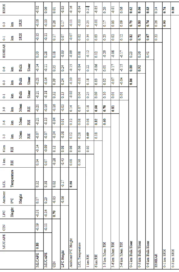
Tabl e 4.2 : C o rr el at ions b et w ee n a s ubse t o f env ir o nm ent al va ri abl es t hat w er e fu rt her i nve st iga ted. C o rr el at io n v al u es g rea te r t h an 0 .50 ar e bo lded.
Chapter 5. Results and Discussion
After storms were discarded due to a lack of representative sites, the storms were categorized as having occurred in tornadic environments or nontornadic environments. Nontornadic and tornadic categories were determined from NCEI’s Storm Events
Database, although this source may have omitted a weak tornado. NCEI’s Storm Events Database was also utilized in order to confirm that storms in tornadic environments produced a tornado; if no tornado was produced, the storm was discarded. This resulted in a final dataset consisting of 123 storms, 40% (n = 49) of which were nontornadic and 60% (n = 74) of which were tornadic. Independence of storm environments was
examined within the dataset; first, each separate event had its own unique sounding, which helps establish independence. Additionally, the number of events from the same day and region were quantified. It is seen that 89 of the storms (72%) occurred on separate days, while the remaining cases were divided into 13 different sets of cases that occurred on the same day (Table 5.1). If the soundings for the storms in these cases were farther apart than 100 km, it was determined that these cases were spatially independent. It was observed that for events occurring on the same day in the same general region, their environments were observed to be independent.
Table 5.1: Independence of cases that occurred on the same day. Asterisks denote cases that contained storms that were both spatially independent and non-spatially independent. In these cases, the first number in the second column is the number of cases that are not spatially independent.
Day Number of Cases Independent by
Space (> 100 km
between soundings)
Independent by
Environmental
Profile
2 March 2012* 2/1 No/Yes Yes
14 April 2012 2 Yes
2 February 2013 2 No Yes
18 March 2013 2 Yes
31 March 2013 2 No Yes
11/12 April 2013 2 No Yes
20 May 2013* 2/5 No/Yes Yes
27 May 2013 2 Yes 17 June 2013 3 Yes 18 June 2013 2 Yes 15 August 2013 2 No Yes 17 November 2013 3 Yes 20 May 2014 2 Yes
While analyzing the data, the mean height of the hail core at the base-level scan was recorded for each time step in order to calculate the mean height of the radar sample volume (HRSV). This metric was also used to categorize storm data in order to
separately consider storms with a mean HRSV below 1 km and storms with a mean HRSV above 1 km in height. These separate height categorizations were needed as the HRSV increases as the beam travels farther from the radar:
(8) where h is the height of the radar beam, r is the range from the radar, a is the radius of the earth, ke is the constant 4/3, and θe is the elevation angle (Doviak and Zrnić 1993). This
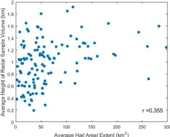
is important from the perspective of hail. More hail might be present with greater altitude due to melting at low levels. Additionally, HAE at the HRSV may not match HAE on the ground as melting might occur between the scan altitude and ground level. The presence of melting hail can modify low-level thermodynamic environments, which can in turn modify storm evolution (e.g., Van Den Broeke 2014). As the mean HRSV increases, so does the measured inferred HAE (Figure 5.1). Approximately 12% of the variability of HAE is explained by HRSV.
Figure 5.1: Average HAE (km2) vs. average HRSV (km). As the average height of the radar sample volume increases, the average areal extent of inferred hail also increases slightly.
Table 5.2 shows the sample sizes from the categories that were developed when the storms were subdivided by mean HRSV and tornadic/nontornadic status. For the Wilcoxon-Mann-Whitney p-tests, the environmental variables were broken into the lowest 25% of values for the entire dataset (LOW), the middle 50% (MID), and the highest 25% (HIGH) in order to see if there was a statistical difference between LOW and HIGH environments (e.g., if hail extent and variability that occurred in LOW-CAPE
environments were different than those that occurred in HIGH-CAPE environments), and to see if extreme events are associated with particular hail characteristics (e.g., are LOW-CAPE environments different than both MID- and HIGH-LOW-CAPE environments).
Nontornadic storms with mean HRSV below and above 1 km, tornadic storms with mean HRSV below and above 1 km, and all storms with mean HRSV below and above 1 km were all used to calculate p-values.
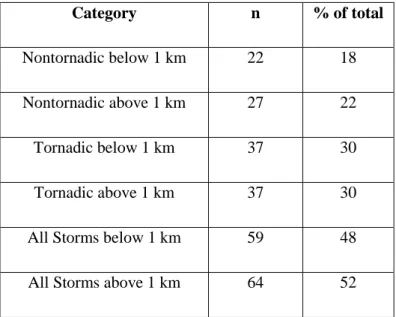
Table 5.2: Sample sizes and percent of total storms analyzed for each defined category.
Category n % of total
Nontornadic below 1 km 22 18
Nontornadic above 1 km 27 22
Tornadic below 1 km 37 30
Tornadic above 1 km 37 30
All Storms below 1 km 59 48
All Storms above 1 km 64 52
The variability in mean inferred HAE, measured by the coefficient of variation, was also calculated for each storm. Values range from 0.162 (variations in HAE were quite small relative to the mean) to 1.314 (variations in HAE exceeded the mean value). Mean hail variability does not differ substantially between tornadic storms (mean
coefficient of variation = 0.56) and nontornadic storms (mean coefficient of variation = 0.62); this result appears to be in contrast with results Van Den Broeke (2016). Kumjian
and Ryzhkov (2008) also found that tornadic storms have more variability; however, they compared the frequency of the presence of hail signatures throughout the mature lifetime of the storm. This study does not take into account when the variability, with respect to the mean, takes place within the lifetime of a particular storm. Van Den Broeke et al. (2008) found that tornadic storms showed high variability of hailfall at low levels, while low variability occurs in nontornadic storms at low levels. It was speculated that lower-level samples would generally have larger mean hail variability; however, there was also no substantial difference in mean hail variability based on the mean HRSV of the storm (Table 5.3).
Table 5.3: Mean hail variability for each category.
Height Tornadic/Nontornadic Mean Coefficient of
Variation Below 1 km Nontornadic 0.66 Tornadic 0.56 All Storms 0.60 Above 1 km Nontornadic 0.58 Tornadic 0.55 All Storms 0.56
Any altitude Nontornadic 0.62
Tornadic 0.56
All Storms 0.58
Analyses were performed on each subset of data to determine correlation coefficients between 1) the mean hail areal extent of storms within a subset to
corresponding values of environmental variables hypothesized to influence the hail areal extent (Fig. 5.2) and b) the variability of hail areal extent of storms within a subset to corresponding environmental variables hypothesized to influence the variability of hailfall within supercell storms (Fig. 5.3). If the correlation coefficient was substantial (|r| ≥ 0.4), areal extent and variability were divided into quartiles (Table 5.4) in order to determine if an environmental variable was strongly correlated to hail characteristics within a specific range of HAE or variability.
Fig. 5.2: Correlation coefficient values calculated for mean HAE (km2) vs. selected environmental variables for a) all environments, b) tornadic environments, and c) nontornadic environments. Storms with HRSV less than 1 km are represented by red dots, storms with a HRSV greater than 1 km by black dots, and all storms combined by blue dots. Dashed lines indicate correlation coefficients with a magnitude of 0.4.
a
b
Fig. 5.3: Correlation coefficient values calculated for hail variability vs. selected environmental variables for a) all environments, b) tornadic environments, and c) nontornadic environments. Storms with HRSV less than 1 km are represented by red dots, storms with a HRSV greater than 1 km by black dots, and all storms combined by blue dots. Dashed lines indicate correlation coefficients with a magnitude of 0.4.
a
b
Table 5.4: Quartile values for mean HAE (km2) and hail variability.
Quartile Mean Areal Extent Variability
Minimum 1.92 km2 0.16 First (25%) 23.63 km2 0.42 Second (50%) 43.93 km2 0.55 Third (75%) 77.97 km2 0.72 Maximum 297.52 km2 1.31 . I. Thermodynamic Parameters
Previous modeling and observational studies have shown that the evolution of storm characteristics is highly associated with upon various thermodynamic parameters such as CAPE; LFC, LCL, freezing level heights; and LFC and LCL temperatures (e.g., Weisman and Klemp 1982; McCaul and Weisman 2001; Kirkpatrick et al. 2007, 2009, 2011). Model simulations have shown that properties of thermodynamic profiles are correlated to an increase in updraft strength, which in turn can lead to an increase in hydrometeor production (Gilmore et al. 2004). These properties include variables such as CAPE, LFC height, and cloud-base temperature (Kirkpatrick et al. 2007, 2009, 2011).
Previous studies suggest a relationship between CAPE and updraft characteristics such as updraft strength (Weisman and Klemp 1982; Kirkpatrick et al. 2007; James and Markowski 2010; Naylor and Gilmore 2014). Observational studies such as Van Den Broeke (2016) have also shown that hail variability is directly proportional to the
environmental MLCAPE value. No correlations of substantial magnitude are found when inspecting all storms, nontornadic storms, or tornadic storms in the dataset, even when taking HRSV into consideration. Neither LOW MLCAPE nor HIGH MLCAPE
environments produced statistically different HAE for all six categories examined, using a Wilcoxon-Mann-Whitney p-test. However, analysis of nontornadic storms with a mean HRSV greater than 1 km show that LOW MLCAPE environments produce a mean variability of 0.393 whereas MID and HIGH MLCAPE environments produce a mean variability of 0.606, which is a statistically significant difference (p = 0.08). Tornadic storms with a mean HRSV less than 1 km in environments characterized by HIGH MLCAPE produce a mean variability of 0.499, whereas storms in all other MLCAPE environments produce a mean variability of 0.567; this difference is statistically significant (p = 0.03).
MUCAPE
Hail production was hypothesized to increase with an increase in most unstable CAPE (MUCAPE), as modeling studies have shown that the CAPE value is directly
related to updraft strength. A theoretical estimate of the peak updraft vertical velocity can be directly related to CAPE by
(9)
although this does not take into account mass loading due to condensate, entrainment of ambient air, or pressure perturbation effects. More hail is expected to be present with greater updraft speeds, as an increase in hydrometeor production is expected with an increase in updraft speed (e.g., Rasmussen and Straka 1998; Gilmore et al. 2004; Van Den Broeke 2014).
When tornadic and nontornadic storms were not differentiated, only storms with HRSV over 1 km show moderate correlation between mean HAE and MUCAPE (r = 0.311). When mean HAE and MUCAPE are compared in nontornadic storms, storms containing a mean HRSV less than 1 km in height have the strongest correlated (r = 0.358). However, MUCAPE differentiates between LOW and HIGH environments for all storms with a HRSV less than 1 km and storms with a HRSV greater than 1 km (p = 0.07 and 0.09, respectively). Storms with a mean HRSV less than 1 km in LOW MUCAPE environments produce a HAE of ~30 km2 whereas HIGH MUCAPE
environments produce HAE of ~56 km2. Storms with a mean HRSV greater than 1 km in LOW MUCAPE environments produce a HAE of ~71 km2 whereas HIGH MUCAPE environments produced HAE of ~109 km2. HIGH MUCAPE environments are statistically different than the combination of LOW and MID environments when considering all storms with mean HRSV greater than 1 km (p = 0.07), whereas LOW MUCAPE environments are statistically different than the combination of MID and
HIGH environments when the mean HRSV is less than 1 km (p = 0.03). These findings are consistent with theoretical expectations: it is theorized that the MUCAPE values are associated with higher updraft speeds (e.g., Brooks and Wilhelmson 1993; Kirkpatrick 2009), and previous work has shown that higher updraft speeds can be associated with higher hail mixing ratio (e.g., Gilmore et al. 2004; Van Den Broeke 2014).
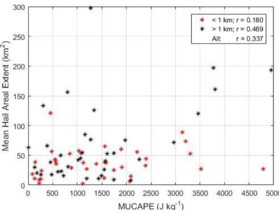
Mean HAE in tornadic storms with a mean HRSV above 1 km have a moderate correlation with MUCAPE (r = 0.469), while all tornadic storms and tornadic storms with a HRSV less than 1 km have weaker positive correlations (r = 0.337 and 0.180,
respectively; Fig. 5.4). Even though there is a moderate correlation between HAE and MUCAPE in tornadic storms over 1 km, no statistically significant differences between environments are present for tornadic storms. It is possible that the positive relationship between HAE and MUCAPE is due to the resulting stronger updrafts, which in turn influences overall hydrometeor production as suggested by previous research (e.g., Rasmussen and Straka 1998; Gilmore et al. 2004; Van Den Broeke 2014).
Fig. 5.4: Scatter plot for mean HAE (km2) vs. MUCAPE (J kg-1) for tornadic storms. Correlation coefficients for storms whose mean HRSV is under 1 km (red stars), storms whose HRSV is over 1 km (black stars), and all storms are listed.
CIN
In the model developed by Van Den Broeke (2016) through multiple linear regression used to predict mean base-scan HAE (Eq. 4), one of the variables included is CIN (J kg-1). Even though this equation, which also includes LFC height (m) and 6-km relative humidity (%) could only explain 51.2% of the HAE variability, the relationship between CIN and mean inferred HAE was further examined in this study. Other
observational studies show that CIN can be predictive of convection including hailstorms (Foote and Wade 1982; Colby 1984).
HAE in both nontornadic storms with a HRSV greater than 1 km and all nontornadic storms is uncorrelated to this environmental variable, whereas nontornadic storms with a HRSV less than 1 km have a slightly stronger negative correlation (r = -0.261). The mean HAE of all storms with a HRSV less than 1 km is uncorrelated to CIN, while all storms with a HRSV over 1 km in height and all storms analyzed have slightly higher positive correlations (r = 0.232 and 0.219, respectively) between HAE and CIN. Different CIN environments are not associated with significantly different HAE inferred at the base level scan for nontornadic storms or all storms whose HRSV was below 1 km. However, in all storms with a HRSV above 1 km, there is a significant difference when comparing LOW CIN environments to HIGH CIN environments (p = 0.05); storms in LOW CIN environments have an average HAE of ~55 km2 while storms in HIGH CIN environments have an average HAE of ~105 km2. Additionally, LOW CIN environments show distinctive HAE signatures when compared to all other environments (p = 0.07, respectively).
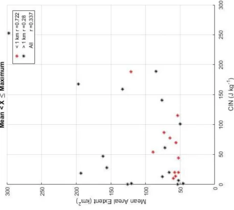
Examining tornadic storms, however, give a different result (Fig. 5.5). Overall, tornadic storms have a moderate positive correlation to CIN with an r value equal to 0.410. Tornadic storms with HRSV greater than 1 km also have a moderate positive correlation to this thermodynamic parameter (r = 0.424), while storms having a mean HRSV less than 1 km have a positive correlation that was slightly lower in magnitude (r
that exhibit HAE greater than the mean value (Fig. 5.6). Defining environments based on the magnitude of CIN also produces significant results when looking at tornadic storms. In tornadic storms with a HRSV below 1 km, LOW CIN environments produce HAE values of ~ 25 km2, while storms in other CIN environments are associated with an average areal extent of ~ 43 km2 (p = 0.04; Fig. 5.7). In general, this result disagrees with prior work, as Van Den Broeke (2016) showed that there was a negative correlation between HAE and CIN (Eq. 4) using a smaller sample of storms. The positive
correlation seen between HAE and CIN may be due to the influence of lowered low-level RH within a layer, as discussed later.
Fig. 5.5: Scatter plot for mean HAE (km2) vs. CIN (J kg-1) for tornadic storms.
Correlation coefficients for storms whose mean HRSV is under 1 km (red stars), storms whose HRSV is over 1 km (black stars), and all storms are listed.
F ig. 5.6 : S ca tt er plot s for mea n HA E ( km 2 ) vs. CI N ( J kg -1 ) f or e ac h CIN b in for torna dic storms. C or re lation co eff icie nts for storms whose HRS V is unde r 1 km (r ed st ars) , storms tha t have a HRS V ove r 1 k m (blac k st ars) , and a ll st or ms ar e li sted f or e ac h b in.
Fig. 5.7: An example of how HAE (km2) varies in association with CIN. a) Storm in the domain of KINX (Tulsa, Oklahoma) on 20 May 2013 at 2030 UTC; CIN is 1 J kg-1 and the mean HAE is 27.30 km2. b) Storm in the domain of KGLD (Goodland, Kansas) on 17 June 2013 at 2029 UTC; CIN is 188 J kg-1 and the mean HAE is 120.75 km2.
LFC Height
Another variable that has been found to have a moderate relationship with mean HAE is the LFC height (Van Den Broeke 2016). A direct relationship between LFC height and mean HAE is hypothesized for a couple reasons. The updraft might be colder on average on days with a high LFC as the updraft will be at a higher altitude.
Additionally, there is a fairly strong positive correlation between LFC height and CIN (Table 4.2) that is influenced by low-level RH. A direct relationship is observed when looking at all the storms analyzed in the present study, although the correlation for this dataset was not as strong as the previous study (r = 0.55 in Van Den Broeke 2016; r = 0.22 in this study).
Storms with a HRSV above 1 km are slightly better correlated (r = 0.312) and the storms containing a HRSV below the 1 km threshold are slightly negatively correlated. LOW LFC environments produce an average HAE of ~48 km2, whereas HIGH LFC environments produce an average HAE of ~126 km2 when considering all storms with an HRSV above 1 km (p = 0.006). Additionally, LOW LFC environments produce
statistically different HAE values than other LFC environments, which produce a mean HAE of ~100 km2 (p = 0.009). Mean HAE values found in the HIGH environments are also statistically different than values found in any other environment, although to a lesser degree as LOW and MID environments produce a mean HAE value of ~68km2 (p
= 0.02).
Interrogation of the nontornadic storms showed that storms with a HRSV below 1 km have the strongest correlation, albeit a negative one (r = -0.384), whereas the mean HAE in storms above 1 km in height and all nontornadic storms have a slightly positive correlation. There is no relationship between all nontornadic storms and LFC height. Tornadic storms follow this same trend (Fig. 5.8), with both the mean HAE of storms with a mean HRSV above 1 km and all tornadic storms having moderate correlations (r = 0.403 and 0.368, respectively); meanwhile, tornadic storms with HRSV below 1 km have slightly weaker correlation between mean HAE and LFC height. Storms containing mean HAE below the mean value show slight correlation to LFC height, whereas when the HAE of the storm was above the dataset mean value, a moderate relationship is seen (Fig. 5.9). This is especially true when looking at all tornadic storms containing a mean HAE greater than the mean value and tornadic storms with a HRSV less than 1 km (r =
0.608). Here as well, when considering values analyzed in tornadic environments with HRSV greater than 1 km, values are different when looking at HIGH and LOW LFC environments. Wilcoxon-Mann-Whitney test p-values show that extreme HIGH and LOW LFC heights were distinguished by mean HAE, as LOW LFC environments are associated with a mean HAE of ~39 km2 and HIGH LFC environments are associated with a mean HAE of ~119 km2 (p = 0.01; Fig. 5.10). Not only are LOW LFC
environments also significantly different than all other environments, which have a mean HAE of ~ 87 km2 (p = 0.02), but HIGH LFC environments are significantly different than all other environments (mean HAE ~50 km2; p = 0.02). These results generally support those found by Van Den Broeke (2016); as the LFC height increased, it was generally closer to the 0°C level (and therefore colder), although there was almost no correlation between these two variables (Table 4.2).
LFC height appeared to exhibit a strong negative relationship to hail variability in previous research (Van Den Broeke 2016), so this relationship was investigated more in depth. The highest-magnitude correlation between hail variability and LFC height is in nontornadic storms containing a HRSV greater than 1 km in height (r = -0.207). This value is negative as found in previous research, although a few of the other data subsets had positive correlations (e.g., variability in nontornadic storms with a HRSV less than 1 km). HIGH LFCs for nontornadic storms with a HRSV above 1 km have statistically less variable HAE (0.53) whereas LFC heights lower than 2625 m have more variable HAE (0.63) (p = 0.07).
Fig. 5.8: Scatter plot for mean HAE (km2) vs. LFC height (m) for tornadic storms. Correlation coefficients for storms whose mean HRSV is under 1 km (red stars), storms whose HRSV is over 1 km (black stars), and all storms are listed.
F ig. 5. 9: S ca tt er plot s for mea n HA E ( km 2 ) vs. LFC he ight ( m ) f or e ac h LF C he ight bin for torna dic storms . Corr elation coe ffic ients for storms whose HRS V is und er 1 km ( re d st ars) , storms that ha ve a HRS V ove r 1 km ( bla ck st ars) , a nd a ll storms a re li sted f or ea ch bin.
Fig. 5.10: An example of how HAE (km2) varies in association with LFC height. a) Storm in the domain of KFFC (Atlanta, Georgia) on 18 August 2013 at 2334 UTC; LFC height is 743 m and the mean HAE is 9.44 km2. b) Storm in the domain of KABR (Aberdeen, South Dakota) on 21 June 2013 at 1855 UTC; LFC height is 3,666 m and the mean HAE is 196.95 km2.
Ambient 0°C Level
The hypothesis that there would be an inverse relationship between the altitude of the 0°C level and the mean inferred HAE was tested. This inverse relationship was hypothesized the understanding that a lower 0°C level would allow onset of melting closer to the surface, resulting in more hail mass surviving to the base-scan level. When studying the relationship between mean inferred HAE of tornadic storms and the
environmental freezing level, an inverse relationship is seen in all three tornadic subsets: all tornadic storms, storms with an HRSV below 1 km, and storms with an HRSV above
1 km (r = -0.274, -0.235, and -0.277 respectively). HAE in nontornadic storms
containing a HRSV greater than 1 km show an even stronger inverse relationship (r = -0.514; Fig. 5.11 and 5.12). There are also moderate negative correlation values when observations are made between the datasets that did not differentiate between tornadic and nontornadic storms. All storms analyzed that had a HRSV above 1 km in height show this relationship (r = -0.300).
Environments containing HIGH freezing levels (above 3850 m) are significantly different than other environments for nontornadic storms and tornadic storms with a HRSV greater than 1 km (p = 0.07and 0.02 respectively). For nontornadic storms, HIGH freezing levels are associated with a mean HAE of ~52 km2, whereas for all other
environments are associated with a mean HAE of ~116 km2; for tornadic storms, HIGH freezing levels are associated with a mean HAE of ~36 km2, whereas for all other environments are associated with a mean HAE of ~80 km2. Additionally, results show a significant difference (p < 0.01) when looking at all storms with an HRSV greater than 1 km. A significant difference appears in the mean HAE between environments containing HIGH and LOW freezing levels (p = 0.005), as ~40 km2 and ~126 km2 of mean hailfall are associated respectively. HIGH freezing levels also produce a significant difference in the amount of HAE inferred when compared against mean HAE in other environments (~97 km2; p = 0.0007).
Fig. 5.11: Scatter plot for mean HAE (km2) vs. 0°C height (m) for nontornadic storms. Correlation coefficients for storms whose mean HRSV is under 1 km (red stars), storms whose HRSV is over 1 km (black stars), and all storms are listed.
F ig. 5.12 : S ca tt er plot s for mea n HA E (km 2 ) vs. 0°C he ight ( m ) f or e ac h 0° C he ight bin for non torna dic storms. C or re lation coe ff ic ients for storms w hose HRS V is unde r 1 k m (r ed st ars) , storms that ha ve a HRS V ove r 1 km ( blac k st ars) , and a ll stor ms a re li sted f or e ac h bin.