warwick.ac.uk/lib-publications
A Thesis Submitted for the Degree of PhD at the University of Warwick
Permanent WRAP URL:
http://wrap.warwick.ac.uk/139956
Copyright and reuse:
This thesis is made available online and is protected by original copyright.
Please scroll down to view the document itself.
Please refer to the repository record for this item for information to help you to cite it.
Our policy information is available from the repository home page.
Reinaldo Castro Souza
A thesis submitted for the degree of Doctor of Philosophy
STATISTICS DEPARTMENT
2
SUMMARY
This thesis describes a new approach to steady-state forecasting models based on Bayesian principles and Information Theory. Shannon's entropy function and Jaynes' principle of maximum entropy are the essen tial results borrowed from Information Theory and are extensively used in the model formulation. The Bayesian Entropy Forecasting (BEF) models obtained in this way extend beyond the constraints of normality and linearity required in all existing forecasting methods. In this sense, it reduces in the normal case to the well known Harrison and Stevens steady-state model. Examples of such models are presented, including the Poisson-gamma process, the Binomial-Beta process and the Truncated Normal process. For all of these, numerical applications using real and simulated data are shown, including further analyses of epidemic data of Cliff et al, (1975).
ACKNOWLEDGEMENTS
To Professor P.J. Harrison, who gave unsparingly of his time and energy to provide the general guidance and suggestions that made this thesis possible, I wish to express my sincere appreciation.
To the Department of Statistics, University of Warwick, ond in particular to Dr. J.K. Ord for supplying the data for the example in chapters 6 and 7, and to Dr. T. Leonard and Mr. I. Liddell for many interesting and helpful suggestions.
To Virginia A. Aguilar for typing the difficult manuscript with great skill and patience.
FOR
Edson, Maria Alice and Maria Carmen
TABLE OF CONTENTS
1 INTRODUCTION
1.1 Scope of the Thesis 8
1.2 Organization of the Thesis 10
1.3 Thesis Terminology and Notations 11
2 ENTROPY FUNCTION
2.1 Historical Remarks 13
2.2 The Notion of Entropy 14
2.3 Definition of Entropy-Discrete Case 16
2.4 Basic Properties of Discrete Entropy 17
2.5 The Extension to the Continuous Case 22
2.6 Other Approaches to the Continuous Case 26
3 JAYNES' PRINCIPLE OF MAXIMUM ENTROPY
3.1 Introduction 33
3.2 Jaynes' Principle 39
3.3 Properties of the Maximum Entropy Density ^2
3.4 Applications 48
3.5 Examples of Maximum Entropy Distributions 51
4 BAYESIAN ENTROPY FORECASTING (BEF)- GENERAL MODEL FORMULATION
4.1 Historical Development of Time Series
52
4.2 Bayesian Forecasting
56
4.3 Bayesian Forecasting Limitations and Proposed Extension
59
4.4 Normal Additive Model; Entropy Results 60
6
4.4.2 Uncertainty Function
4.5 Bayesian Entropy Forecasting System 4.5.1 Model Foundations 4.5.2 General Assumptions 4.5.3 System Evolution 4.5.4 Exponential Approximation 4.5.5 Model Formulation 4.6 BEF - Properties
4.6.1 Mormal Additive Model 4.6.2 Non-Additive Normal Model 4.6.3 Parameter Prediction 4.6.4 System Evolution
4.6.5 Steady State Model-Definition
4.6.6 Goodness of Fit-Relative Entropy Criterion 4.6.7 Aggregate likelihood for Estimation of Hc"
4.7 Sufficient Statistic Specification
5 STEADY STATE POISSON-GAMMA MODEL 5.1 Introduction
5.2 Entropy of the Gamma Variate
5.3 BEF Poisson-Gamma System ; Model Description 5.4 Limiting Form of the BEF Poisson-Gamma Model
Applications and Discussions
61 64 64
66
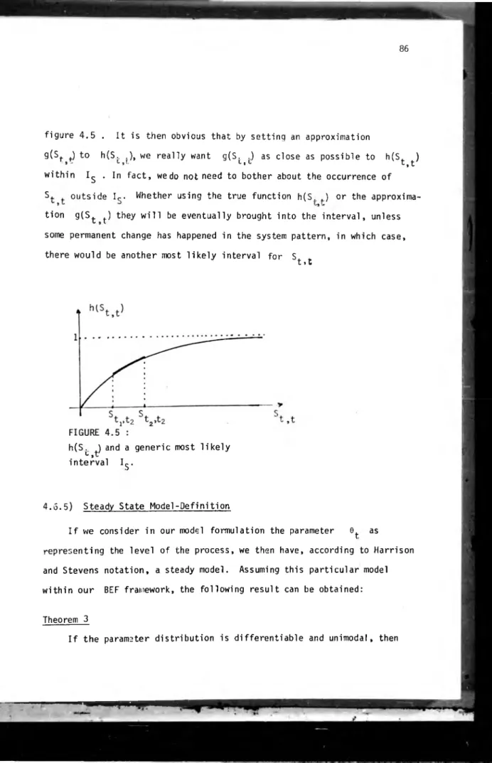
67 72 75 79 79 81 83 84 8688
92 93 97 98 100 103 5.5 1056 POISSON-GAMMA MULTI STATE MODEL 6.1 Introduction 109 6.2 The Model 110 6.2.1 Information a Priori 111 6.2.2 Updating System 113 6.3 Collapsing Procedure 115 6.4 Case Study 120
6.4.1 Preliminary Data Analysis 121
6.4.2 Results 123
6.4.3 SM and MM Comparison 125
7 STEADY STATE BINOMIAL-BETA MODEL
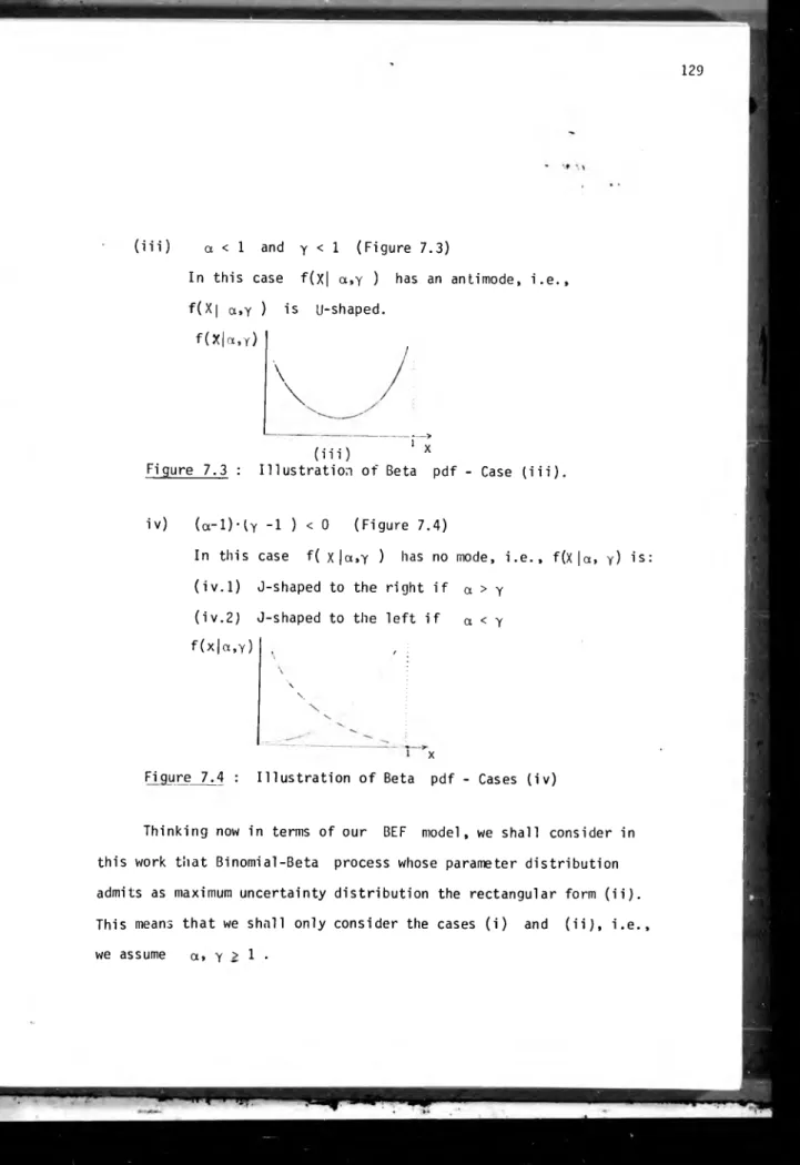
7.1 Introduction 126
7.2 Beta Variate Characteristics 127
7.3 Entropy of the Beta Variate 130
7.4 BEF Binomial-Beta System ; Model Description 131
7.5 Limiting Form of the Binomial-Beta BEF 131
7.6 Applications 135
8 STEADY STATE TRUNCATED NORMAL MODEL
8.1 Introduction 141
8.2 Truncated Normal Distribution 113
8.2.1 Definitions and Characterizations H 3
8.2.2 Properties 117
8
8.4 Bayesian Analysis for the Truncated Normal Distribution 155
8.4.1 Parameter Posterior Distribution 8.4.2 Predictive Distribution
156 159
8.5 BEF Truncated Normal System ; Model Description 161
8.6 Applications 165 Appendix A 169 Appendix B 173 Appendix C 179 Appendix D 182 Appendix E 190 Appendix F 196 Appendix G 212 References
220
field of forecasting. The first major advance, of course, was Box and Jenkins' very clear formulation of forecasting models in 1970. However, their solution of the least square prediction problem was still shackled to the fundamental ideas of Wiener and Kolmogorov. Undoubtedly this was one of the most important contributions to the subject.
At almost the same time, Harrison and Stevens developed an important approach to forecasting using important results of Kalman and Bucy, already extensively used in Control Theory problems, together with Bayesian
statistical theory. This approach gave rise to the so called "Bayesian Forecasting Methods" which offered something quite different from the Wiener and Kolmogorov theory. It is well known that the three basic assump tions on which all the previous forecasting methods are based are:
- stationarity of the underlying process,
- mean square prediction error as a forecasting criterion, - predictor as a linear function of past observations.
These were partially overcome by the advent of the Bayesian approach. For instance, the stationarity of the underlying process is not required and also, by its distributional predictive nature a criterion of optimality other than the mean square error is possible.
Despite the above improvements and its simple, elegant formulation, the Bayesian approach as it stands still has its limitations. For instance, the models are still linear, where the observation noise and parameter disturbance
10
are additively related to the observation and system equations respectively, and (from the linear least square property of the Kalman filter) it is efficient only for the Normal process.
These two restrictions consitute the prime motivation for this disserta tion. Our principal aim in this thesis is to develop an extension of Harrison and Stevens' approach in which the constraints of linearity and normality are not required. With this extension we are not merely satisfy ing the four essential basic foundations of the Bayesian Approach, namely:
(i) Parametric formulation.
(ii) Probabilistic information on the parameters at any given time,
(iii) Sequential model definition.
(iv) Uncertainty as to the underlying model,
but furthermore, we include the following two properties:
(v) Non-linear general formulation.
(vi) Unrestricted to any sort of distribution.
However, the original target of an unconditional formulation applicable to any kind of model has not been entirely reached. In this thesis we discuss only steady state models: a particular but important subclass of all models. On the other hand, we feel that this work has gone an appreciable way towards the original goal and further extensions, which might include a broader class of models such as the linear growth, seems quite feasible following the same argument.
a crucially important measure of uncertainty and Jaynes' principle of maximum entropy. By the incorporation of Shannon's entropy into a Bayesian framework, the steady state linear normal model can be redefined in terms of the entropy function and, using the fact that entropy is an unrestricted measure of uncertainty, the extension follows naturally.
1.2) Organization of the Thesis
The thesis could be classified into three main parts. Part I (Chapter 2 and 3) is devoted to the definition and characterizations of the entropy function, as well as its main properties. In chapter 3 we show the mathematical formulation of Jaynes' principle of maximum entropy to assign the least
prejudiced probability distribution for a random variable and some of its most important properties.
In Part II (Chapter 4; the theoretical Bayesian Entropy Forecasting (BEF) model for a steady state system is defined and described, starting from the steady state linear normal model. It also includes a brief survey of time series modelling and a summary of some of the most important forecast ing methods.
Part III (Chapters 5 to 8) deals with some applications of the model to different processes such as:
- Poisson-Gamma single state process (Chapter 5). - Poisson-Gamma multistate process (Chapter 6). - Binomial-Beta single state process (Chapter 7). - Truncated normal process (Chapter 8).
12
For each of these we show the relevant numerical results concerning their application to simulated and real data. Of particular interest is the analysis of the measles epidemic data in chapters 5,6 and 7.
Finally, the thesis is complemented by 7 appendices (A to G) containing mainly tables and figures related to the numerical results of the applications in Part III.
1.3) Thesis Terminology and Notations.
Throughout the thesis we use several notations, some of them standard and some others newly defined for the particular topic under consideration. However, in order to avoid confusion we try to clarify any unfamiliar nota tion on its first appearance and thereafter where necessary. On the other hand, we make use of some standard abbreviations such as: r.v. (random variable), pdf (probability density function), IR (real numbers), R+ (positive real numbers), Z (integers).
All the probability distributions that we shall use in the thesis are defined in terms of density functions over Euclidean spaces with respect to Lebesgue measures, lie adopt either "p" or "f" as a generic symbol for a probability density function. Also, we use the conventional distinction between a random variable and its realisation as a value, i.e. capital letters X,Y, etc. representing random variables and lower case letters x,y etc. representing their realised values.
To conclude, the term "parameter" is extensively used in the thesis to mean the random variable representing the "level" of the steady state process. The Greek letter 0, sometimes suffixed 6t> is the generic
symbol we use to represent for the level to avoid misunderstanding with parameter* of a probability distribution, which are usually represented by the conven
tional Greek letters a, 6,
y ,
p, a etc. lie reserve the term Yt for the random variable representing the process observation in the model formulation.14
CHAPTER 2: ENTROPY FUNCTION
2.1) Historical Remarks
The word
cntAopy
has had a long and controversial evolution in science. In the original greek its literal meaning isVianA (omnallon
and it was with this literal sense that in 1850 Clausius [ see Tribus 1961a and 1969 ] introduced the wordcntnopy
in his work as a quantity associated with transformations from work effects to heat effects in thermodynamics. It was only at the beginning of this century that it was used again, this time in a completely different subject, in the works of S. Boltzmann and M. Planck in Statistical Mechanics. They proposed a general procedure for determining the distribution of the total energy of a system among its elemental single components, when the assumption is made that all such elemental single components are in dependent and identically distributed. TheBoltzmann H-fiunctloni
which originated from their work, is used a great deal in statistical mechanics [ Planck. 1950; Mackey 1957 ].
It was, however, only in 1948 that it became universally known due to the work of C.E. Shannon in the context of communication theory
[Shannon & Weaver, 1949 ]. In his work Shannon developed thoroughly a new and useful axiomatic quantitative study of the acquisition, production and transmission of information, named afterwards
Shannon’ A
Tn(omatlon Thcoay
. This work produced again another definition of ancntAopy (¡unction',
in this case, a quantitative measure of the missing information in a message or in a probability distribution. As remarked by Shannon, Information Theory is very broadly based, in the sense thatit applies to all kind of systems for which the given information is in complete, that is, for those systems where uncertainty is involved. More generally, information theoretic concepts are relevant to any field in which inductive probabilities are useful, for inductive proba bilities arise whenever the given information is not sufficient to permit deductive inferences. Although ever since Shannon, information theory had grown into a broad, highly developed body of knowledge, only in 1957 did E.T.Jaynes show that Shannon's entropy function had a deeper meaning and in fact, as a disciple of statistical mechanics, he demons trated that both
zntA-oplU
were in fact the same thing and therefore not mere analogies. [Jaynes, 1957 & 1958; Tribus, 1961a ]2.2) The notion of Entropy
Let 5= ( ç., Çg.... tn ) be the set of possible outcomesc's in some physical experiment. Suppose also that at first we do not know anything more about the experiment and the occurrence of any of the possible out comes. Then, suppose we are told that the outcome is more likely to occur. Provided the given information is reliable, our previous state of knowledge must change and it would be useful to have a quantitative measure for the information newly acquired. Putting the problem in a quantitative form, suppose that our original state of knowledge and our state of knowledge after receiving the information are represented by probability assignments P^* and P respectively; in other words, we have two probability schemes:
16
where: S is the sample space (assumed finite) F is the field of events
P° = (p°> P2 .... P°) i P°= P r o b i ? ^
P =(p1. P2 .... Pn ) ; P ^ Prob( c . | Inform.)
The above set up for the problem allows us to introduce the concepts of information and entropy. Firstly if we are interested in a quanti tative measure for the information provided by the new data relative to our prior knowledge, we have to take into account the two probability distributions P° and P, representing respectively our state of un certainty before and after gaining the information. We finish up with a quantity I(P,P°) known as
Incarnation -in
PaeJLatioe. to
P° or simplyInCarnation .
Secondly, the problem could be formulated in a slightly different way, where we could only be interested in an absolute quantitative measure of the information. The quantity proposed by Shannon, known asShannon'i EnViopy,
is a measure of the missing information or the amount of uncertainty in a single probability assignment. Put in this way, we can clearly see the basic conceptual difference between Information and Entropy. In the first we measure quanti tatively information in a probability assignment relative to a prior assignment, while in the second we have the same sort of measure in an absolute way. We shall point out later that Shannon's entropy, although simpler and easier to work with, suffers from the defect that it can not be consistently generalised from discrete to continuous probability spaces. On the other hand I(P,P°), being a relative measure of in formation does not suffer from this defect. Attempts have been made toformulate a clear, simple and consistent measure of information or even to develop a general theory in terms of information rather than entropy. Among the various works in this particular area we cite:
Vincze, (1972); Hobson,(1971); Kolmogorov,(1956); Kul 1 back,(1959) ¡Jaynes, (1968), Vincze,(1959 & 1965) and Perez,(1957).
2.3 Definition of Entropy-Discrete Case
Let Sn denote the set of all finite discrete probability dis tributions (P=(p1,p2 .... pn); p.j> 0; i = l,2.... n; E p ^ l } .
In other words, P may be regarded as an experiment having n possible outcomes x^ ,x2 .... xn with probabilities p(x^)= Pj , p(x2 )=
= p2 ,... ,p(xn )= pn . Then,
the entropy o(> the. cUitAtbutlon
P , or a measure of how uncertain we are about the outcome of the experiment is given by:H(P)= Hipj.pg....pn)= ifnpi> = - I p. £npi --- --- (2.1) for PeSn and all n=l,2,... and also, with the usual convention that
whenever p ^ O we set pi f n p ^ O .
Theorem: (Fundamental Theorem of Information Theory ).
Up to a constant of proportional ity, the function H(P) given in equation (2.1) is the only function satisfying the three require ments for being a measure of uncertainty of an assignment of probability P :
i) Continuity on p.
equal (p.=l/n). That is, with equally likely events, there is more choice, or uncertainty when there are more possible events.
i i i ) Consistency:
H(p1,p2 ,...,pn )=H(p1+p2 ,p3 ,. ,Pn)+ (Pi+P2 )-H ( ^ P2
V p2
or, if a choice is broken down into two successive choices, the original H should be the weighted sum of the individual values of H.
Proof: The original proof of the theorem is found in Shannon and Weaver, (1949-Appendix 2), and some elaborated proofs can be found
in Mathai & Rathie, (1975); Feinstein, (1958) and Akaike, (1971).
2.4 Basic Properties of Discrete Entropy
Apart from the properties (i) to (iii) above, Shannon's entropy has many other properties and characterisations, some of which we show below. For a thorough treatment of these properties, see for instance: Shannon & Weaver, (1949); Mathai & Rathie, (1975) and Kul 1 back, (1959) .
Using the index n in H(P) to denote the entropy of P=(p1 ,p2 ,...,pn ) i.e., Hn(P)=H(p1,p2 .... pn ) ; we enumerate the following further properties of Hn(p):
1) Non-Negativity:
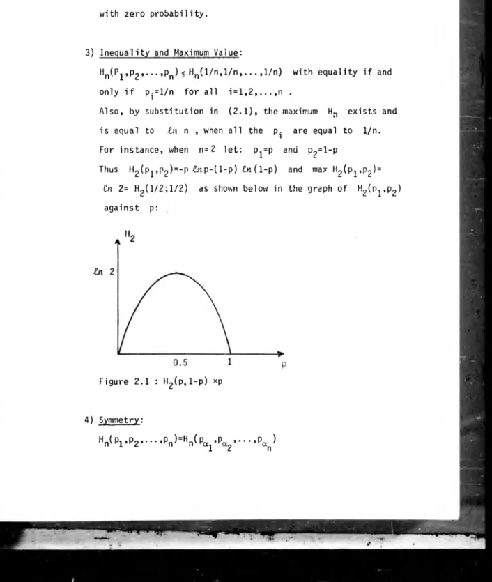
3) Inequality and Maximum Value:
Hn(P1,p2 ,...,pn ) < Hn (l/n,l/n.... 1/n) with equality if and only if p^l/n for all 1 = 1,2....n .
Also, by substitution in (2.1), the maximum Hn exists and is equal to
in
n , when all the p^ are equal to 1/n. For instance, when n = 2 let: Pj=p and p2=l-pThus H2 (p1,p2 )=-p £np-( 1-p)
in
(1-p) and max H2(p^,p2) =in
2= H2(1/2;1/2) as shown below in the graph of H2(Pj,p2)against p: 4*
Figure 2.1 : H2(p,1-p) xp
4) Symmetry:
20
where (a , ocg,..., an ) is any arbitrary permutation of the indices (1,2.... n). From the above, we can state that the entropy is the same whatever the order in which the possible outcomes are labelled.
5) Joint Events: Let:
pl=(PλP2....Pj) eSn
P2=(P?-P2....p£) ^
where Sn and Sm are classes of all finite discrete probability
1 p
distributions P1 and
PL
respectively..Pi
P=(P1,P2 ) = (pn ,. lm* ' ' " P n l .... ,pnm^ e^nm p .. is FiJ the probability of joint occurrence of i with probability
1 2
p. and j with probability p^ . S nm as above,
Then:
Hnm<p) iHn(pl)+ Hm (F>2)
Alternatively, the entropy or uncertainty of a joint experiment is less than or equal to the sum of the entropies of the in dividual experiments. It is equal if and only if the indivi dual experiments are independent. 6
6) Coherence:
but it is worth mentioning in its own right. As a measure of uncertainty in a probability assignment, for any change toward equalisation of the p^(loss of information or increase of the uncertainty), the entropy increases.
Formally, if we have:
P=(Pr P2 .... Pn) and P*=(P|,P^,...,P* )
and 2 |p.-l/n|i 2 |p*-l/n |, then:
i 1 1 1
Hn(P) <Hn (P*)
7) Conditional Entropy Let:
P ,P ,P, P^jbeas defined in property (5).
(xj.Xg,...,x^) and (x^.Xg.... x£) the possible outcomes
1 2
of experiments P and P respectively. 2
2
p(j|i) the conditional probability of the outcome Xj given that the outcome of experiment with distribution P^ is
xj; i=1,2.... ri and j=l,2,..., m.
1 2 1
Then, the conditional entropy of P" given P is:
In
p (j | i)} 2 p. .in
p(j|i) i ,J JFrom the above and the results of property (5), we obtain:
Verbally, the sum of the amount of uncertainty in the probability assignment P* for the first experiment and the amount of un certainty for the conditional experiment is the entropy of the joint experiment. Also, the above inequality states that if there
is any dependence between two experiments, there is always a gain of information (or a decrease of the degree of uncertainty) of one of the experiments, given the knowledge about the outcome of the other.
8) Invariability: Let:
X be a discrete random variable which can assume values Xj,x2 ,...,xn with probabilities Pj=P(x=x.), i=l,2,...,n
H represents the entropy of the experiment under consideration (instead of using the H(P) notation of (2.1)).
Y= t(x) a one-to-one transformation of the random variable X and Hy its associated entropy.
Then, this property states that:
Hy = Hx = H(P)
That is, the formula (2.1) for the entropy of an experiment is invariant with respect to any bijective transformation of the variable; it is not dependent on the domain of the variable, but depends only on the probability distribution.
- and characterisations of Shannon's entropy function. The prime objective of describing these few properties was to clarify the ideas behind the entropy function as an absolute measure of the amount of uncertainty in a single assignment of a probability distribution for an experiment. For a detailed mathematical and probabilistic study of all the properties and characterisation theorems of Shannon entropy, we refer mainly to Mathai & Rathie, (1975 ) .
2.5 The Extension to the Continuous Case:
If in the definition of section 2.3 we let the number of possible outcomes n for a given experiment increase indefinitely so that P tends to a continuous probability density function p(x) of a continuous random variable XeX, it would be natural to try to define the entropy as a limiting case of the entropy for discrete distributions (2.1). However, if we do so, we obtain:
H [p(x) ]=- p(x) X
In p(x). dx - lim EAx..p(x.). In Ax.
Axi“K) i 1 1 1
Accordingly, the expression for H [p(x)] diverges as Ax^-*- 0 whatever the value of the first term. Instead of defining H[p(x)] as a limiting case, Shannon suggests that we should simply define the entropy for a continuous random variable xeX with probability density function p(x) purely by analogy as follows:
?A
H [p(x) ]=- E {£np(x)
}=-P(x) /
p(x ). £np(x).dx--- (2.2)
and for a random vector x =(xj,x2 ,...,xn )T e / 1 and associated p(x):
H fp(x) ]=- E Unp(x)} =-
‘ ' P(x)
» • • • > p(x).£np(x).dx1.... dxn— (2.3)
The entropy as defined in (2.2) or (2.3) has nearly all the important properties described in the last section and as such, is a measure of the amount of uncertainty in the probability assignment p(x) for a continuous random variable X. However, as remarked by Shannon, the continuous entropy function (2.2) or (2.3), is not general in the sense that for some particular cases, properties (1) and (8) are not attained. Let us first consider the lack of invariance under a monotonic change of variable.
Let:
X be a continuous random variable, XeX, with pdf px(X) . Y=g(x) be a monotonic transformation of X.
Thus, Y is also a continuous random variable, Y eY, with pdf
is the jacobian of the transformation, substitution in the above equa tions gives: Py (Y). Then, by (2.2): H (X)=- px (x).£npx(x). dx and H y X Py (Y).£npy (Y).dy
or, after expanding the logarithm: H
Y
Px(x)-[
Px(x)+£n|J|]. dx
and finally: H y = Hy - E { £n|J|} Px(x) (2.4)Equation (2.4) clearly shows the dependence of the entropy of Y on the Jacobian on the transformation, confirming the lack of invariance under the change of variable
X v g(x).
This restriction led Shannon to give an extra interpretation to entropy. For both, the discrete and the continuous case (2.1) and (2.2) measure the randomness or the amount of uncertainty involved in the assignment P or p(x) to a discrete or a continuous random variable X respectively. However, the measurement in (2.1) is completely absolute in the sense that no matter what random variable is describing the experiment, the entropy is always the same. On the other hand, the entropy in (2.2) or (2.3), measures the uncer tainly relative to the coordinate system (sample space) adopted, i.e., relative to the random variable used. It is however important to remark that, in most of the applications, we in fact are interested in the increase or decrease of the amount of uncertainty of systems whose randomness is changing continuously in time. In this case the Jacobian term of (2.4) would appear in both entropies, cancelling out eventually. This means26
that the lack of invariance of the measure (2.2) is not a restriction to its use.
With respect to the possible situations in which the entropy
is negative, the problem can be easily circumvented by adopting a scale of measurement for the entropy for each kind of distribution under considera tion.
Let us consider, for example, the normal distribution: If X=N( p, a2), then: H =
¿n
/2nea^
A
It is quite clear from the above that H can assume any value A
in R and also that zero entropy does not mean perfect information or a degenerate distribution. In fact, Hx =0 for o 2= Og = (2ire)~^ means that there is still some uncertainty (though small), about the outcome of the experiment. We could for instance, adopt this state of uncertainty as the standard one and then compare subsequent values of H x with this standard. Any positive H x would indicate that we have a broader distribution than Og and a negative H x would indicate a still narrower distribution than ag , that eventually tends to -°° as a 2 approaches zero.
2.6) Other Approaches to the Continuous Extension
Although we shall use the simplified Shannon's entropy (2.2) or (2.3) in our model formulation later on, it is worth mentioning some other attempts towards a general definition of entropy. A lot of different approaches to the problem have been put forward after Shannon and in all of them, a slightly different interpretation of
a meaiuAe
unc.eAtcu.nty
is made in order that a unique function is obtained for both the discrete and continuous cases. We briefly describe a few of these approaches and point out their similarities.We start with the work by Hobson Q Hobson, 1971; Reza, 1961 and Pinsker, 1964 ]. He sets up the problem by first defining a relative measure of information for discrete distribution and then, extending it to the continuous case.
Let:
S = { cn > be a finite sample space.
P^,P be a pair of probability distribution assignments in S before and after gaining some evidence about the outcome of the ex periment respectively, where:
P°= (pj.p^.... P° > ; p!j = Prob (c ; i=l,2,...,n
P = (pj.pg.... pn } ; p^= Prob {ç . | Inform.}; i = l,2,. ,n
Then, instead of defining a measure of the information missing in a single probability assignment as Shannon did, Hobson defines a quanti tative measure for the information provided by the new data which he called
In iom atton In P nelattoe to P°
or simplyIniom atton
as:I(P,P°)= E Un(p./p?)} =
Z
Pi ..En(p,/p°)---- (2.5)P 1 1 i=l 1 1 1
Hobson shows that the above quantity, while measuring the gain of information instead of the missing information, satisfies all the
28
main properties of Shannon's entropy and that it is easily extended to the continuous case, preserving the properties.
The extension from discrete to continuous variables is first made by extending the measure in (2.5) from a finite discrete to an infinite discrete sample space. For this case I(P,P°) becomes:
oo
I(P,P°) = 2 Pi £n(p./p<? ) ... ... (2.6)
i=l 1 1 1
Assuming S to be a segment of the real line (a< x< b) and P°&P a pair of continuous probability assignments with densities f°(x) and f(x); the information in P relative to P° , or the information in f(x) relative to f°(x) is easily obtained using (2.6) and, taking limits of discrete partitions in [a,b] , we obtain:
I(P,P°)= I[ f(x), f°(x)] = E (£n [f(x)/f°(x)J } = b
= | f(x). £ n ^ . d x ---- (2.7)
3 f°(x)
The relative measure of information for a continuous distribution in (2.7) , as opposed to the absolute measure of missing information in (2.2), is non negative and invariant under a one-to-one transforma tion X-*-Y = g(x).
Hobson then proceeds by introducing a concept similar to Shannon's entropy, defining a measure of missing information or un certainty in the probability assignment P, by considering the prior
assignment P° and the assignment Pm , corresponding to the maximum knowledge about the outcomes c's.
Since I(Pm ,P°) is the maximum information possible relative to P° and I(P,P°) is the actual information relative to P°, the missing information necessary to attain the maximum knowledge state Pm (missing information or
unc.eAtcu.nty in P
), is:U(P;Pm ,P°)= I(Pm ,P°)- I(P,P°) ---- (2.8)
Again, the above quantity has all the properties required for a measure of uncertainty in P; it is applicable to either the discrete or the continuous case but has the disadvantage of requiring the know ledge of two extra probability assignments namely the prior P° and the maximum state of knowledge Pm .
Another interesting approach towards a general definition of entropy is that of Vincze (1959), (1965) and (1972). He starts by giving a rather different interpretation to Shannon's entropy in discrete finite space. Vincze interprets entropy as a measure related ndtto the probability distribution, but to a decomposition of the space of the elementary events.
if Dn =(A1 ,A2>...,An ) is a decomposition of S={ ?2.... and PM = Ip-=P(A.); i= 1,2.... N ; Z p. = l }, then the entropy
n i i i=1 i
associated with the particular descomposition is given by:
N
Hn = -E Unp.}= - Z p..£np.
PN i = l
30
where e [0,£n N ] The above measure of uncertainty is in fact Shannon's entropy (2.1) . However, instead of considering for measuring the uncertainty associated with the decomposition , Vincze suggests an equivalent measure called information denoted by 1^ that has the property of measuring uncertainty by means of informa tion, defined by:
IN= E i£n N .pi}= £nN-HN - (2.10)
PN
where I^e [0,£n N ] .
As remarked by Vincze, one of the main advantages of using (2.10) instead of (2.9) is that under mild conditions concerning the continuous distribution, although tends to infinity, the remaining information 1^1 will have a finite limit. In fact, when we pass from the discrete to the continuous case, the above information M . (also known as comple -mentary entropy), tends to a limit called I-divergence in the literature but interpreted in this context as the information of a continuous random variable XcX and given by:
I(X )= E
Un
^ } = { f(x).In
^ . dx - - - - (2.11) f(x) <J>(x) X <t>(x)where f(x) is the probability density function of X and <|>(x) is the
cUMAibutcon
0&
ouain tzA U t,
defined by a reasonable partition of X.Some interesting applications of the use of the I-divergence in finding confidence intervals for unknown parameters of various density functions, by a suitable choice of the distribution of interest are shown in Vincze,(1965).
Finally, we briefly mention Jaynes' set up for the same problem [ Jaynes, 1958
*,
1968 ] .In his work, Jaynes is only interested in finding an absolute measure of uncertainty for a continuous distribution. In fact, he departs from (2.1) for the entropy of a discrete distribution. He then points out the restrictions of (2.2) for measuring the same thing for the continuous case by emphasizing once more that (2.2) is not a result of any derivation. He proceeds with his argument by taking the entropy of a discrete distribution to the limit obtaining:
H[p(x)]=- E
{In
p(x) m(x)
p(x).£n m(x)
. dx - (2.12)
where m(x) is an invariant measure, proportional to the limiting density of discrete points. In this case, both p(x) and m(x) transform in the same way under a change of variable and so, h[p(x)] of (2.12) is an invariant measure. In fact, an extra interpretation given to m(x) by Jaynes is that:
apaAt ¿Aom a nosumLiitng constant,
m(x)a pAtoA duAtAibu-tion deAcAtblng compieXe. ignorance about
X.We conclude this section by remarking that whether we use Hobson's information (2.7), Vincze's I-divergence (2.11) or Jaynes'
H [p(x)] (2.12) density function prior assignment three approaches are preserved.
for measuring the randomness in the probability assigned to a continuous random variable a subjective
f°(s), *(x) or m(x) is required. However, all are general, in the sense that all desirable properties
Let us consider the simple form of Bayes' theorem for a discrete random variable , written as:
p(x1 |DK)ctp(0|x1K)- p(x.j |K)
One of the main controversies in using the above theorem has been the question of how to assign prior probabilities p(x.|K), based only on the information K prior to any observation. We could for instance, break the situation up into mutually exclusive and exhaustive possibilities and use the
p/UnctpZe. ofa tm u ^ ic ie n t xeaiou
in such a way that no one of them is preferred to any other, i.e., assigning aurUioxm p/Uox .
However, situations occur in which we are given some other relevant evidence that increases our state of knowledge in such a way that the uniform prior assignment turns out to be inappropiate. In this case, with this extra prior information, we have some reason to prefer some possibilities to others. Our aim is to assign a probability which is, in some sense, as uniform as it can be subject to the available informa tion. It shouldipxzad out
all over the sample space, not assigning zero probability to any situation, unless the available information really leads to this conclusion.So, the aim of avoiding unwarranted conclusions leads us to search for a reasonable function that measures
thz uni&o/unity
of a probability distribution which could be maximised subject to the constraints which represent the available information. In fact, this function which we seek34
measures the
unceAJtcUnty
or¿gnoànnce
about a situation whose maxi misation, subject to the constraints, would give us the minimally prejudiced assignment of a probability distribution.In this chapter we will show that the only function that gives the minimally prejudiced distribution required in the above set up of our problem is the Shannon entropy developed in chapter 2. Before we proceed with the mathematical formulation of this problem, we show first through some simple examples that other functions, such as the variance or E {p .}
p i (or E {p(x)} for the continuous case) which also measure the
p(x)
spread, uniformity or uncertainty of a probability distribution do not give the minimally prejudiced distribution we want.
Let us first consider a die throwing experiment in which we are given the information:
i) The die has six sides with'’f- = i"spots on the ith side.
ii) The average number of spots obtained in a previous long series of throws was 4.5 (instead of 3.5 for a fair die).
Based on these two pieces of information, we want to assign a minimally prejudiced probability distribution to this experiment;
P (fi = i > = P i , i= 1,2.... 6
and let us suppose first that we cltoose the variance of the required distribution as the objective function, that is:
Max £ (f.-4.5) . p, i = l 1
subject to: 6
Z
f.p. = 4.5 ... - (3.2) 1-1 1 1 6 I Pi = 1 ; p^>
0, i = l....6 ---(3.3)The solution to this maximisation procedure is:
P {fj) = 0.3 ; P {fg}= 0.7 ; P ff2 } = P i i y = P(f4> = Ptf5>= 0
On the other hand, if we use Shannon entropy (2.1) in place of (3.1) above as the objective function we would obtain by its maximisation subject to the constraints (3.2) and (3.3):
P (fj) = 0.055 P{f2 ) = 0.079 P{f3) = 0.114 P{f4 )= 0.165
P {fg} = 0.240 P{fg} = 0.347
It is easy to show that the solution to the above problem (using for example the Lagrange multipliers) as a function of X is:
Pj = (8-3X)/ 6 p2 = 1/3 P3(3X-4)/6
Plotting these probabilities against X we get:
!1ax -E {p^j before adjustment Max -E {p^j after adjustment for for negative probabilities. negative probabilities.
In figure 3.1 above the curves for Pj and p3 clearly show that for 1 <
% <
4/3 and 8/3 < s 3 respectively, the probabilities are negative. To replace this impossibility we introduce the extra constraint that p^ > 0 ; i= 1,2,3 and we obtain the final result as plotted in figure 3.2 .As a matter of comparison, let us solve the sane problem by using Shannon entropy H (p^) instead of F(pi) in (3.4). Using again the same argument, the following distribution is obtained:
38
p.j= exp{(2-i)a} /(1+2 cosh a) ; X = (e2a + 2ect+3)/(e2a+ea+l)
or, after simplifying:
p2= / [4-3(X - 2)2 ]/ 9 - 1/3 ; Pj=(3 -X -P2 ) /2 and
P3 = ( X -1 -P2 ) /2
Maximum entropy distribution.
2
Although the Max -j p^ shows a big improvement over the maximum variance distribution (see the die experiment of the previous example), for certain values of X it assigns zero probabilities and that is again jumping to conclusions not present on the given information. On the other hand, the maximum entropy distribution (figure 3.3) represents in fact the least prejudiced probability distribution for
Xi that meets the objectives of our problem. Another point in favour of the entropy is that the extra constraint p^ > 0, which must be introduced in the first case, is automatically included in the entropy
The two simple examples discussed, illustrates how the entropy function is in fact a consistent measure of uncertainty,and that it leads to least assignment of probability distribution for a random variable.
In the next section we show the mathematical set up of the problem by postulating the principle and the general solution.
3.2) Jaynes Principle of Maximum Entropy:
We now formalise the procedure to find the least prejudiced probability assignment introduced in the last section. Originated in 1957 by E.T. Jaynes, the rationale behind the proposed principle of maximum entropy is that the probability distribution desired has maximum
uncertainty (minimum information content) while representing some explicitly stated known information.
The principle is general, in the sense that it always gives a minimally prejudiced probability distribution, although, as stated by Jaynes, (1958) and (1968), the information given concerning the random variable in question, should be a
testab le, piece of information
, defined as follows:A
piece- o f information concerning a random variable
Xi s calle d
te sta b le i f for any proposed probability assignment
p(x)¿or
X,there i s a procedure which w ill detennuie unanbiguously whether
p (x )does or doer not agree with the given inform ation.
■
40
among all the possible testable information, Jaynes considers in his formalism only those concerned with averages of functions of the random variable being studied, since this class of information is the most common one we find in practical problems. But the principle as a whole, is applicable to any kind of testable information.
We now formulate the principle and its mathematical set up mainly for the continuous case. The discrete development is similar and has been extensively explored in the literature. For comprehensive develop ments and illustrative examples see: Jaynes, (1958,1963 and 1968); Hobson, (1971); Tribus, (1961a & 1969) and Goldman,(1953).
The principle:
The minunalZij pfiejadiced pfwbabtlUty ciistfUbution Is th at ivlUch
imx.imises the entaopy Subject to constficUnts supptied by the.
givente sta b le ¿n^ofwiation.
Put this way, Jaynes' principle encompasses the well known
pfvincA.ple
0
|Stn iu iilc te n t fieason
as a special case. However, there is no way of proving Jaynes formalism. As pointed out by Tribus,(1961 a) it should rather be interpreted as an axiom for a system of inductive logic. To see this point more clearly, let us consider the schematic representation for the principle as shown below:input information
concerning r.v. X .
Jaynes formalism * (llax. Entropy proce
dure)
output
(Max. entropy distribu tion for X )
Accordingly, if the output conclusions agree with posterior observations of the experiment, we conclude that the input information is coherent and sufficient for our purpose. On the other hand, an output not agree ing with the observations, forces us to admit that the input information is not correct and finally, a vague output corresponds to insufficient input information.
Bearing in mind this rationality behind the principle, let us now proceed with the calculations in order to obtain the maximum entropy distribution.
Ue are faced with the so-called isoperimetric problem of the calculus of variations that could be formulated generally as:
Find p as a function of Xc X such that the function I (p ) defined as:
where ^(X.p) and Ki are preassigned functions of X,p and constants respectively. From the calculus of variations, the p(x) which maximises I(p) is obtained by solving the equation:
I(p) = F(X,p)• dx X
(3.7)
is maximised, subject to the conditions:
4
>j (X,p) - dx= K. ; i = l,2.... n - - (3.8) X42
Where X , i= 1,2,..., n are adjustable constants (Lagrange multi pliers), calculated by direct substitution of p(x) into constraint equations (3.8).
He can now easily adapt our problem to the above set up as follows:
XeX is a continuous variable
p(x) is the probability density of X , to be obtained by maxi mising the entropy (2.2), i.e., by setting F(X,p)=-p(x
)-In
p(x) in (3.7).<t>i (X , p )= g.j(x)- p ( x ) ; i = l , 2 , . . . , n ; where g ^ x ) are known functions of X, whose expectations with respect to p(x) are known and equal to - constraint equations.
p(x)- dx = 1 is the normalising constraint. X
Taking these quantities into the general solution (3.9) (with an additional adjustable constant Aq due to the normalising constraint) we obtain after simplifications the maximum entropy density p(x):
n
p(x)= z • exp {-
s
A.g.(x)} ; z= exp { -An } ... (3.10)i = l 1 1 u
(The discrete case is similarly set by substituting summations for integral s).
3.3) Properties of the Maximum Entropy Density:
We now s t a t e and prove some o f the s t a t i s t i c a l properties of
Where , i= 1,2,..., n are adjustable constants (Lagrange multi pliers), calculated by direct substitution of p(x) into constraint equations (3.8).
We can now easily adapt our problem to the above set up as follows:
XeX is a continuous variable
p(x) is the probability density of X , to be obtained by maxi mising the entropy (2.2), i.e., by setting F(X,p)=-p(x
)-In
p(x) in (3.7).<f>i(X,p)= gi (x) • p(x); i = 1,2.... n ; where g^(x) are known
functions of X, whose expectations with respect to p(x) are known and equal to Ki - constraint equations.
p(x)- dx = 1 is the normalising constraint. X
Taking these quantities into the general solution (3.9) (with an additional adjustable constant A„ due to the normalising constraint) we obtain after simplifications the maximum entropy density p(x):
n
p(x)= z • exp {-
l
A .g. (x)} ; z = e x p { - A 0 } ... (3.10)i=l 1 1 0
(The discrete case is similarly set by substituting summations for integrals).
3.3) Properties of the Maximum Entropy Density:
We now s t a t e and prove some o f the s t a t i s t i c a l p rope rtie s of
43
can be derived from the maximum entropy approach, we only show those that specifically concern our work.
We conclude the section by stating and proving theorem and a corollary, important for our model formulation. A parallel develop ment for the discrete case can be found in chapter 5 of Tribus,(1969).
i) Partition Function Properties:
"The mean, variance and covariance of the random variables g.j(x) ; i= 1,2,..., n are related to the Lagrange multipliers
Aj, Ag>• • •« *n and the
PaAtttion Function
(zeroth Lagrange multi plier Aq ; also known asPotential Function)
by:Taking p(x) of (3.10) into the normalising constraint, we get: E {9,- (x)} P(x) (3.11) Var {g - (x)} = ---- ~ p(x) 3A-(3.12) P(x) Cov igi(x)• (3.13) i ,j= 1,2.... n Proof: X or: e • dx (3.14)
Differentiating (3.14) with respect to A , we obtain: or: e"0 3Aq 8 A . 1 ^ 0 = _
1
3Ai j X £ *k M x)-—” 0 Q k e . e g.j(x). dx - £ Ak gk(x). g.j(x). dx using again (3.10): ‘0 ( — = - j g^x). p(x). dx 3A„ 3 A . - E { g (x) } = -K. P(x) 1 1To prove (3.12) we follow the same argument by differentiating (3.14) twice with respect to A.. We obtain, after simplication:
- £ H g j x ) . (— ^ ) 2 + v 3Ai
'
" O k e e 3Ai X . g^(x). dxUsing (3.10) & (3.11) we obtain:
32Ar
E2 {g.(x)> + - ^
5
-= E {g2 (x)} and (3.12) followsp(x) 1 3A2 p(x) 1
Finally, differentiating (3.14) with respect to Ai and A . and taking into account (3.11) and the fact that:
cov { g,(x) g.(x)} = E { g,(x) g,(x) } - E (g.(x)}. E (g,(x) }
n M 1 J nivl 1 J p(x) nfxl J
p(x) ' J p(x)
expression (3.13) follows immediately.
45
ii) Maxi mum Entropy Properties:
"The maximum entropy value is related to the Lagrange multipliers A. and the expectations ; i = l,2,..., n by:
Hm = Hm( Ar X2 ....A j = Hm (K1fKp ... K„)
n' nr 1* 2 ’ •(3.15)
3H
3^7 = A. ; i = l,2....n’
where Hm is the maximum entropy value.
- (3.16)
Proof:
Taking p(x) (equation 3.10) into H(p) (equation 2.2) we obtain:
Hm = H [p(x)] = - { [ -aq - E gi(x).
X.
]. p(x). dxby expanding the terms within brackets:
Hm = Ag + z A.. E . { g,.(x) }= An + z A.. K.
1 P(x) 1 0 : r i
Since the potential function as given in (3.14) can be expressed as a function of the A-'s alone and consequently the K/ s in (3.11), H can be expressed as a function of the A-'s only ; i = l,2,..., n.
m i
Conversely, regarding the K ^ s as the independent variables, the a.j1 s could be solved for K ^ s and an expression for Hm as a function of the Ki 's alone is obtained.
To prove (3.15) let us consider the differential element dHm from the above:
n n
dll = dAn + Z K ■. dA, + Z A. . dk.
Using the fact that aq= xQ ( x ^ a2>..., a ), dxQ can be written as:
dxQ =
3A-. 3A« 3A~ n 3A~
3X7 d X1 + 3X7 dX2+" ,+ 3A I d n ^ n = . s1 ^ r - d*i i=l i n
and from (3.11) : dXQ = - £ K1-. dx.
Therefore:
n n n n
dH = - Z K..dA.+ z K..dA.+ Z A..dK.= Z A.. dK. m i=i 1 1
1=1
1 1 i=i 1 11=1
1 1and (3.16) follows.
i i i) Theorem:
"The maximum entropy distribution (3.10) is a member of the regular case exponential family of distributions"
Proof:
If the random variable X has a probability density function which is a member of a regular case exponential family of distributions indexed by
written as
parameters § = ( »•••» en )» then its pdf can be
n
p(x ,
0
) = A(0 ). exp {l
Q.( 0 ). R .(x) }i = l 1 1
where, for 1 = 1.2.... n:
^ ( x ) are functions of X alone and not of
0
X-47
Let p(x| o ) be the parametrised probability density function corresponding to p(x) of (3.10). Taking p(x| e ) into (2.2) it is clear that after integrating out X, we are left with a function of e alone ; i.e.
Mni ='i p(xl 0 )-'en p(x I §)• dx = Hm ( 0 ) X
or, using (3.15), llm = Hm (
0
, K , a)where: a =(a1> A2 ... An ) and K »(Kj.Kg,..., Kn >
using (3.16) we now obtain:
3H ( e, K, x)
’-■= Xi /. Ai = A ^ 0 , K)= X1( e ) ---- (3.17) l
i= 1,2,..., n .
That is to say, the Lagrange multipliers a^ , i= 1,2.... n
are functions of e alone (since K are specified constants independent of x) and not of X.
Also, from (3.14) and taking into account (3.17) we can write for tiie partition function Aq:
a q = Aq ( 0 ) ... (3.18)
Then, using the fact that g^(x) ; 1 = 1,2.... n are by assumption functions of X alone and not of e and the results (3.17) and (3.18) the maximum entropy density has the form of p(x,
0
) above and the theorem follows.iV) Corollary
The specified functions g^x) ; 1 = 1,2,..., n are such that for a given random sample x :( x.,x2 .... x[() from this distribution [ t g ^ X j ) , r g2 (Xj).... r gn (xj) ] ; j = 1,2,..., N , comprise a set
of joint sufficient statistics which is minimal if none of them is redundant.
3.4) App1ications:
In this section we give a brief scrvey of the most recent
and important applications of entropy and Jaynes Principle of Maximum Entropy to various subjects. Particularly in the statistical context, although not yet completely organised as a statistical method, the cited principle has proved to be of great help in many situations, mainly in Bayesian Statistics, where it provides a constructive criterion for setting up prior probabilities distributions on the basis of partial knowledge where conventional methods do not apply.
If it had been our aim to describe a complete survey of these applications we would have to start by giving an extensive list of its various uses in the fields of Communication Theory and later in Statistical Mechanics, lie however interpret these subjects as the
Entropy PaAznti
and as such we are only concerned with the use of entropy in other fields.i) Mathematical Ecology:
In the subject of Ecology Shannon's entropy has provided an entirely different way of measuring diversity in populations, assumed to contain an indefinitely large number of individuals that could be classified into a finite number of species.
49
Assuming also that each individual belongs to one and only one class and that is the probability of an individual being in the species group C.j, i = l,2,..., n ; then Hl p ^ ^ , . . . , pn ) provides a measure of the diversity of the population [ Pielov, 1966,1967 and 1969; Brown & Disk, 1975 ] .
ii) Reliability Studies:
In reliability studies of equipment which is maintained over a long period of time through replacement of components, the lifetime behavior associated with these models ranges from complete determinacy to complete uncertainty. The associated probability of survival, hazard and number of replacements can be obtained by maximising the entropy associated with the randomness [Tribus, 1962 ; Flehinger & Lewis, 19591.
iii) Thermodynamics:
Using entropy it is possible to show that the general maximum entropy formalism is intrinsically related to the experimentally measured quatities of a system in thermodynamic equilibrium. For instance, if Hc is the experimentally measured entropy of a system and Hs the corresponding Shannon's entropy then Hs < Hg , with equality if and only if the probability distribution in Hs is that one which gives maximum H . [Jaynes, 1963 a ; Tribus, 1961a, 1961b ] .
iv) Statistical Inference:
The problem of decision making in the face of uncertainty can, by its very nature , be formulated and solved by using the notion of entropy as a criterion for setting up prior proba! ility assignments.
Once the loss function has been specified, our uncertainty as to the best decision arises solely from our uncertainty as to the state of nature and so, the entropy. We refer mainly to : Jaynes, (1963b); Dutta.( 1966); Edwards.(1972); Vasicek, (1974) and Barnard, (1951).
v) Stock Market Prices:
A very general probability distribution of future stock price in a market can be obtained by use of Jaynes formalism. The maximum entropy distribution of future stock price for an investor having specified prior information is general and agrees with past observations of the market prices. [ Mandelbrot & Taylor, 1967 ; Cozzolino & Zahner, 1973 j .
vi) Econometri cs :
In the field of Economics, Shannon's entropy has also been used a great deal. In Econometrics for instance, certain estimation me
thods such as least square, weighted regression, maximum likelihood are used and can be shown to be optimal in the Information Theoretical sense. We refer specially to: Tintner,(1960); Tintner & Sastry, (1969) and Theil,(1967).
vii) Model Identification-Time Series:
The application of entropy in the time series context is due to Akaike,(1971, 1972, 1974, 1977 a, 1977b, 1977c and 1978) and Tong,(1975a and 1975b). Akaike succeeded in deriving a 1-dimensional statistic for selecting an optimal model from a class of competing models by using
the generalized entropy of a distribution with respect to another (or the Kul 1 back-Leibler mean information for discrimination between two distributions ; Kullback, 1969). Akaike's criterion, (also known as A.I.C. - Akaikes information criterion), is particularly important in estimating the order of auto regressive and/or moving average models.
3.5) Examples of Maximum Entropy Distributions
We conclude this chapter with some illustrative examples of maximum entropy distributions, obtained by the use of Jayne's formalism techniques developed in the previous sections.
g^x); i = l .... n E ig^x;} . X
g ^ X
g j =0 ; j=2,... ,n
E (gj) = x IR+ Exponential (A)
g:= x g2=
In
Xgj= 0; j=3.... n
E {g^} = a E {g2 } = 6
IR+ Gamma (a,6)
gj=
In
X g2=l n (
1-x) gj-0 * j-3,... ,n E {g^} =a
e ig2 } = Y CO.ll Beta (a ,y ) gx= x g2= x2 9j~0» j-3,...,n E {g1)= u E (g2 }=y2 +o2
IR Normal (y,o2 )IR+ Single Truncated
Normal (y,o2 ) [a,b] i a,b
fin i te
. Double Truncated Normal (y,a2 )
GENERAL MODEL FORMULATION
4.1) Historical Development of Time Series
Throughout this section we shall consider Khintchine's and Kolmogorov's interpretation of time series [Khintchine, 1932 ; Kolmogorov, 1933 ]. According to them, if we accept the broad view of a times series Yt as a set of observations ordered sequentially in time, then, it is also possible to interpret it as:
i) A stochastic process whose variables Y^, Y2 ,..., Yp are observed at equispaced time intervals tj,t2 .... tn .
ii) An n-dimensional probability distribution Y. . It is with that interpretation of time series in mind that we start our brief historical development of time series.
The first attempt towards an explanation of the functional form of a time series, dates from the very beginning of the last century. This was due to Joseph Fourier who claimed the approximation of any time series by a combination of sine and cosine curvers.
It was only at the beginning of this century that Fourier's idea was used again by Schuster, (1906). He succeeded in estimating periodicities in time series by introducing periodogram analysis. However, the limitations of use of the periodogram analysis [Beveridge,
1922 T, together with the great advances in probability theory and statistics experienced at the beginning of the twentieth century,
provoked substantial developments in time series analysis. Starting in 1927
53
with Yule and complemented in 1938 by Wold [ Yule, 1927 ; Wold, 1938; Walker, 1931 and Slutzky, 1937 ], the concepts of autoregressive and/ or moving average (AR, HA, ARMA) schemes were introduced, which proved to be the most general linear representation for a stationary time series. Wold did not give much attention to the parametric estimation of this new scheme. The first methods for estimating the parameters of an AR, HA, ARMA model are due to Kolmogorov,(1941) and Man & Wold,(1943).
In order to follow our chronological description, it is worthwile considering now the important work by Wiener in estimation theory.
Around 1940 Wiener working in the field of communication theory, developed new techniques for filtering a signal at the receiver whose transmission has been distorted by a white noise process [Wiener, 1940 ]. In other words, if Y* is a signal transmitted at time t and is the random
disturbance in the transmission of Y^ , Wiener assumed that the signal ★
received is additively related to Y^ and , i.e. :
Yt = Y* + for all t = 1,2,...
where the are assumed to be independent identically distributed Gauss i an random variables , with E { vt } = 0 and F { v | } = o 2 . Wiener developed an estimation procedure for the white noise in the frequency domain for a continuous process so that an optimal filter was obtained (The analytical solution to the Wiener-Mopf integral equation). The discrete version of Wiener's work was independently developed by Kolmogorov by assuming that a stationary time series has a representation as above, thus the reconstruction of the real process Y^ could be obtained.
From that point, both Wold's autoregressive and/or moving average scheme in the time series context and Wiener's filter theory in the engineering context were developed a great deal, but it was only with the advent of computational facilities that a real boom occurred. The first major step forward was the work by Kalman and Bucy in 1950 [ Kalman, 1960 and Kalman & Bucy, 1961 ] which proposed a solution to the Wiener-Hopf integral equation by transforming it into its equi valent differential equation, but working in the time domain. The
recurrence relations and updating equations obtained - the
Ka&mn FLltM.,
as it is nowadays known could easily be solved by use of digital computers. Ever since Kalman, the new filter theory was developed and applied to different areas of engineering, particulary, in Control Theory [De Russo et al, 1967 ; Sage & Melsa, 1971 and Meditch, 1969 ].Wold's scheme however, had its real great boom ten years later with the important work by Box and Jenkins [Box & Jenkins, 1970 ]. Box and Jenkins' contribution, undoubtedly has started a new era in time series and forecasting. Using the facilities of digital computers mentioned above, they proposed a new strategy for the construction of a set of linear stochastic equations, describing the behavior of a time series, whether stationary or not. Briefly, they assume that the given series can be reduced to stationarity by differencing a finite number of times, i.e. by determining the stationary series w^. by:
w t = (1 " B)d Yt
where:
55
B is a backward shift operator on the index of Y^ , such that:
■ V ' t - i • » ’v V z
It is then assumed that the stationary series can be represented by an ARMA model of the form:
p q
( 1 -
z
<t> .¡B1) w. = ( 1 - £0
■ BJ) ai=l 1
Z
j=l J rwhere:
$. are the autoregressive parameters (1 = 1,2,..., p)
9
. are the moving average parameters (j=l,2,..., q)a is a white noise sequence, with constants variance a2
or, in terms of Y^:
(1-
T.
♦iB1)(l-B)d Y. = (1 - s o-Bj ) a ;1=1 1 1 j=l J
known as an ARIMA (p,d,q) model.
Finally, the well known Box and Jenkins procedure to fit a model of the above form to a given set of data, consists of a three-steps iterative cycle procedure: identification (p,d,q values), estimation (
0
. and a2 ), diagnostic checking (validity of the identifiedi J a
model) and then the forecasting stage. A lot of applications and further developments of the method have been extensively published, lie only refer to some of them. [ Hakridakis, 1974; Gilchrist, 1976; Souza, 1974; D'Araujo, 1974; Brubacher, 1976 and Cleveland, 1972 3.
Almost at the same time as Box and Jenkins, a new and important approacl) for forecasting was put forward by Harrison and Stevens L Harrison & Stevens 1971, 1976a and 1976b ]. They were in fact pioneers
of the use of the Kalman filter results in a time series forecasting context. The so-called
Bayesian Forecasting Syitem
orAdaptive.
Forecasting
based on a joint use of Kalman results and Bayesian Statistics, offered a great improvement over the existing methods. Instead of consider ing a simple fit to past data in order to predict the future in a purely automatic way, they are mainly concerned in their method with the actual present information and its effects on the future. Since our model formula tion is an extension of the above cited method, we dedicate the next section to a brief summary of Harrison and Steven's method, as well as the justi fication of our proposed extension.We conclude this section by mentioning the recent
S tate Space
Forecasting
proposed by Mehra,(1976, 1977a, 1977b, 1977c). He used only the Kalman Filter results for forecasting single and/or multiple time series, in other words using only the past data in order to get the model identification and the parametric estimation in a very automatic way. Although the method is very general and easy to use, it has the great disadvantage that the past history of the process is an essential require ment due to its non-Bayesian nature.4.2) Bayesian Forecasting
In this section we give a brief description of the Kalman Filter- Bayesian approach for forecasting as proposed by Harrison and Stevens, pointing out the main advantages accruing to this new approach.
57
The model formulation is based on a complete parametric description of the process, which is incorporated into a dynamic linear set of equations describing:
i) process observation
ii) parameter evolution
In its general form, the Dynamic Linear Model (DLM) is:
Observation equation : Yt = Ft et + vt - - - (4.1) Parameter evolution equation: et= G 9t_j + w t - - - - - - (4.2)
where :
Yt is an (m*l) vector of observations
°t is an (nxl) vector of unknown parameters
Ft is an (mxn) matrix of independent variable (known at time t) G is an (n xn) system matrix
Vt is an (mxl) vector representing the observation noise; vt * N(0,Vt)
wt is an (nxl) vector representing the parameter noise; w t * N(0,Wt)
t is the time index (t=l,2,... )
The parameters are easily updated from tin« to time by use of the Kalman Filter updating equations, in other words, if: