Measurement 2018, Vol. 78(5) 781–804 ÓThe Author(s) 2017 Reprints and permissions: sagepub.com/journalsPermissions.nav DOI: 10.1177/0013164417722179 journals.sagepub.com/home/epm
Item-Focused Trees for the
Detection of Differential
Item Functioning in Partial
Credit Models
Stella Bollmann
1, Moritz Berger
2, and Gerhard Tutz
3Abstract
Various methods to detect differential item functioning (DIF) in item response models are available. However, most of these methods assume that the responses are binary, and so for ordered response categories available methods are scarce. In the present article, DIF in the widely used partial credit model is investigated. An item-focused tree is proposed that allows the detection of DIF items, which might affect the perfor-mance of the partial credit model. The method uses tree methodology, yielding a tree for each item that is detected as DIF item. The visualization as trees makes the results easily accessible, as the obtained trees show which variables induce DIF and in which way. In the present paper, the new method is compared with alternative approaches and simulations demonstrate the performance of the method.
Keywords
partial credit model, differential item functioning, recursive partitioning, item-focused trees
Introduction
In psychometric tests, it is generally assumed that measurement properties are stable across individuals, a property that is known as measurement invariance (Millsap, 2012). However, it might occur that different groups of people react differently to
1
Universita¨t Zu¨rich, Zurich, Switzerland
2
Department of Medical Biometry, Informatics and Epidemiology, University Hospital Bonn, Bonn, Germany
3
Ludwig-Maximilians-Universita¨t Mu¨nchen, Munich, Germany Corresponding Author:
Stella Bollmann, Universita¨t Zu¨rich, Binzmu¨hlestraße 14, Zurich, 8050, Switzerland. Email: [email protected]
the same test, which threatens the validity of the measurements. Also, test fairness is violated if tests lead to different conclusions for distinct groups of people. Differential item functioning (DIF) means that measurement invariance is violated on the item level. More precisely, DIF is present if one or more items are significantly more diffi-cult for one group than for the other after controlling for the underlying ability or trait.
One can distinguish between uniform and nonuniform DIF.Uniform DIFmeans that
the difference between the groups is constant across levels of the latent continuum of the individual. If it is dependent on the ability or trait of the personnon-uniform DIF is present. DIF detection procedures can also be classified into item response theory (IRT) methods and non-IRT methods. The IRT methods, also called parametric meth-ods, are those in which an IRT model is used for the detection of DIF. For an over-view of IRT methods and non-IRT methods, see Holland and Wainer (1993), Magis, Be`land, Tuerlinckx, and De Boeck (2010) and Penfield and Camilli (2006).
The basic idea of traditional DIF detection procedures in both dichotomous and polytomous IRT models is to prespecify two groups of persons and then determine whether item parameter estimates differ between these groups. The first method that was used for the detection of DIF in IRT models was the likelihood ratio (LR) test (Andersen, 1973). An alternative approach that can be used for any kind of IRT mod-els isLord’s chi square test(Lord, 1980). While this test is restricted to the compari-son of two groups, its extension by Kim, Cohen, and Park (1995), thegeneralized Lord test, can be used for more than one focal group. A third approach is theRaju method (Raju, 1988), which is based on the idea that the difference between the shape of item response curves (IRCs) between two groups indicates DIF. Further test statistics for parameter differences between pre-specified groups were suggested by Thissen, Steinberg, and Wainer (1993) and Holland and Thayer (1988). These classi-cal methods have in common that they are limited to few sub-groups that need to be pre-specified by the user. Moreover, it is hard to consider more than one DIF-indu-cing covariate at a time.
More recently, two strategies were proposed for the detection of DIF in Rasch models that is generated by multiple covariates and for which sub-groups do not have to be pre-specified. The first strategy uses regularization methods to handle the abun-dance of parameters in the model. Tutz and Schauberger (2015), Magis, Tuerlinckx, and De Boeck (2015) and Thissen et al. (1993) used penalized likelihood estimation, whereas Schauberger and Tutz (2016) proposed boosting methods to obtain regular-ized estimates. The second strategy is to use recursive partitioning techniques, often called tree methods. One needs to distinguish between two quite different forms of tree methods in DIF detection. In the method proposed by Strobl, Kopf, and Zeileis (2015), called RaschTree, the covariate space is recursively partitioned to identify regions of the covariate space in which item parameters differ. In the investigated regions, a parametric latent trait model that includes covariates is fitted. Regions are suspected to be relevant if their parameter estimates differ strongly. A disadvantage of the method is that it detects regions of the covariate space that are linked to DIF, but does not automatically detect the responsible items. The alternative recursive
partitioning method propagated by Tutz and Berger (2016) focuses on the detection of the items that are responsible for DIF. Unlike the RaschTree, it uses recursive par-titioning on the item level, not on the global level. Since the method is able to flag DIF items it is referred to as item-focused trees.
For polytomous models, in particular the partial credit model, DIF detection methods are less common than for dichotomous models. Some methods are proposed in Penfield and Camilli (2006). For further concepts, see also Penfield and Algina (2003), Penfield (2007) and Penfield (2008). A method that competes with the approach considered here is the extension of the RaschTree to the partial credit model proposed by Komboz, Strobl, and Zeileis (2018). It will be considered in more detail in the section Comparison of Recursive Partitioning Methods.
The objective of the present paper is the development of item-focused trees for the partial credit model. In the next section, the notation and the basic model will be introduced. In addition, we present an illustrative example. The tree algorithm that is used is given in detail in the subsequent section. In the penultimate section, we show results of wider simulation studies. In the final section, we discuss further possible extensions of our modeling approach.
DIF in Partial Credit Models
In the following, we considerIitems with ordered categories andPpersons. For sim-plicity, we assume that the number of categorieskis equal across items.
The Partial Credit Model
Let Ypi2 f0, 1,. . .,kg,p= 1,. . .,P,i= 1,. . .,I, denote the ordinal response of
per-son pon item i. The partial credit model (PCM), which was proposed by Masters
(1982), assumes for the probabilities
P(Ypi=r) = exp(Prl= 1updil) Pk s= 0exp( Ps l= 1updil) , r= 1,. . .,k,
whereupis the person parameter and (dil,. . .,dik) are the item parameters of itemi.
For notational convenience, the definition of the model uses implicitly
P0
k= 1updik= 0. With this convention, an alternative form of the model is P(Ypi=r) = exp(rupPrk= 1dik) Pk s= 0exp( Ps k= 1updik) :
The link to the binary Rasch model becomes obvious when one considers responses in adjacent categories. Given response categoriesrandr1, the presentation
log P(Ypi=r) P(Ypi=r1)
=updir, r= 1,. . .,k, ð1Þ
shows that the model is locally a binary Rasch model with person parameterup and
item difficultydir. The properties of the model can be visualized by IRCs that show
the probabilities of a response in categoryras a function of the person parameterup.
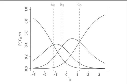
An example of the IRCs for one item with four categories is displayed in Figure 1. From the curves, it is immediately seen that forup=dirthe probabilities of adjacent
categories are equal, that is,P(Ypi=r) =P(Ypi=r1). This means that the IRCs of
adjacent categories intersect atup=dir. Therefore, the parametersdir can be seen as
thresholds between categoriesr1 andr. In Figure 1, the thresholds are marked by dashed lines at the intersections of the curves. For example,Ypi= 0 means that
cate-gory 0 was chosen and no threshold was exceeded. The score Ypi= 2 implies a
response which exceeds thresholds 1 and 2 but fails threshold 3. For more details regarding the model see also Masters (1982), Masters and Wright (1984) and Andrich (1978, 2013, 2015).
Item-Focused Trees for the Partial Credit Model
In model representation (1), the linear predictor for personpand ther-th threshold of itemiis given by
hpir=updir:
In item-focused trees, the predictor is successively modified by allowing different predictors in different regions of the covariate space. In the simple case of a continu-ous variablex, one allows a split into the regionsfxcgandfx.cgat split-point c. A tree is grown by successive splitting of one of the available variables at one of the corresponding split-points. The root is the top node without splitting and the ter-minal nodes represent the identified partitioning of the covariate space.
For a more concise description, letxT
p= (xp1,. . .,xpV) denote a vector of
measure-ments on personp. Starting from the root, the predictor that is fittedfor one item i and all persons has the form
hpir=up gir(1)I(xpvcv(i)) +gir(2)I(xpv.c(vi))
, r= 1,. . .,k, ð2Þ
where I() denotes the indicator function with I(a) = 1 if a is true and I(a) = 0 otherwise. This means that itemishows DIF generated by thevth variable. The item has parameters gi1(1),. . .,gik(1) in the left node I(xpvc(vi)) and parameters gi1(2),. . .,gik(2) in the right nodeI(xpv.c(vi)). The split-pointc(vi) defines the regions
that are used for itemiand has to be chosen in an appropriate way. Since an own tree is built for each item, the split-points typically vary over items.
Further splitting means that one of the nodes, for example the left nodeI(xpvc(vi)),
I(xpvc(vi))I(xps c(si)) and I(xpvc(vi))I(xps.c(si)),
wherec(i)
s is a new split-point for variablexps and itemi. For each region, one again
obtains new parameters for the item. Naturally, only items should be split that carry DIF and the variables and their split-points have to be selected carefully.
In the following, the model abbreviation PCM-IFT will be used for item-focused trees based on the PCM.
An Illustrative Example
Before presenting the fitting procedure of the proposed model in detail (see the next section), we give an illustrative example. The example is used to demonstrate how a tree that is obtained by PCM-IFT looks like and how it can be interpreted. The data considered here are the responses of 1000 subjects on the 8 items of the subfacet Fantasyof the factorOpenness to experienceof the German version of the NEO per-sonality inventory revised (NEO-PI-R; Ostendorf and Angleitner, 2004). The 1000 subjects were randomly drawn out of the 11,724 cases of the norm data set. The sam-ple was taken to obtain standard values for the test manual. Each of the items has five categories (fromstrongly disagreetostrongly agree). Additionally, the data set comprises the two variables age and gender. There are 382 males and 618 females between 16 and 81 years of age.
Figure 1. Item response curves (IRCs) for one item with four categories. The item parameters are marked by dashed lines.
The major domainOpenness to Experienceis described in the manual asthe active seeking and appreciation of experiences for their own sakeand the subfacetFantasy asreceptivity to the inner world of imagination(Ostendorf & Angleitner, 2004).
Using PCM-IFT, two of the eight items were selected as DIF items. The two items with DIF are the following:
Item 3: I have an active and lively fantasy life.
Item 6: When I feel that my thoughts are drifting off into daydreams, I usually become busy and start to focus on a task or an activity. (R)
The (R) behind item 6 indicates that this item was reverse coded. This means that strong agreement to this question indicates a low level of fantasy. For simplicity, all reverse coded items have been recoded before the analysis. Therefore, for all analy-ses a high value on this item means the person disagreed with it.
Item 3 was only split once in covariate gender. The resulting tree is shown in Figure 2 (upper panel). At the terminal nodes, the four threshold parameters for the respective partition are given. It is seen that for both groups, thresholds are not ordered indicating that a higher latent trait is required for passing the second thresh-old than for passing the third threshthresh-old. This effect is slightly more extreme for males than for females. Also, for males an even higher latent trait is required to pass the fourth threshold.
Item 6 was split twice with regard to gender and age. The first split was found for variable gender and within the sub-group of females it is distinguished between
younger women (age 40 years) and older women (age .40 years). The resulting
tree is shown in the lower panel of Figure 2. Similar to Item 3, in none of the termi-nal nodes the thresholds are ordered. The main difference between the three groups is the variation of the threshold parameterd61, which is highest for females with age
40 years and lowest for females with age .40 years. For the latter, this threshold parameter was even below24 and is therefore not visible in the figure that is trun-cated at24. Since the item is reverse coded, this means that for older females, the probability was particularly low to pass the last threshold from agree to strongly agreefor this question. Looking at the answers, we see that in this group (terminal node 3) only 2 persons out of 133 had chosen the last category.
The illustration shows that items with DIF can simply be identified by using the proposed PCM-IFT. The resulting trees are easily interpretable and show which vari-ables and split-points determine DIF.
Fitting Item-Focused Trees
In this section, a detailed description of the fitting procedure for the proposed PCM-IFT is given.
The Partial Credit Model as a Generalized Linear Model
Under usual assumptions, the partial credit model can be embedded into the frame-work of multivariate generalized linear models (GLMs). Let the data be given by (Ypi,xp),p= 1,. . .,P,i= 1,. . .,I. For the item responses, one assumes a multinomial
distribution Ypijxp;M(1,ppi), where pTpi= (ppi1,. . .,ppik) with components ppir=P(Ypi=rjxp). The link function of the GLM can be derived from model
equa-tion (1) and has the form
g(ppir) =hpir= log P(Ypi=r) P(Ypi=r1)
= (1(pP))Tu(1(rk))Tdi, ð3Þ
where uT= (u1,. . .,uP), dTi = (di1, ,dik) and 1(rk) denotes the unit vector of lengthk
with a 1 in componentr. To ensure the identifiability of model (3) one parameter has to be fixed. In the following we setuP= 0. By defining the whole parameter vector bT= (uT,dT1,. . .,dTI), the PCM can be written in the closed form
hpir=zpirb,
wherezpiris the design vector for personp, itemiand thresholdrthat has to be
spec-ified accordingly.
Computation of Estimates
Estimates for Model (3) can be obtained by using the flexible R-package VGAM
(Yee, 2010, 2014). Function vglm() allows the estimation of so-called vector
GLMs (Yee and Wild, 1996). One simply needs to specify the design matrix as described above and estimation can easily be obtained. In addition, one can make use of the argumentparallel() to specify category-specific item parameters. In the following algorithm, which yields the PCM-IFT, this estimation procedure serves as a building block in each iteration.
Fitting of Trees
When growing trees, two decisions have to be made in each step. One has to deter-mine the best split due to an optimality criterion and has to decide if the split is rele-vant or not. In contrast to alternative approaches, the trees are not pruned to an adequate size after building an oversized tree. By early stopping, the size of the trees is controlled directly.
To determine the first split, one examines for all the items, all the variables and possible split-points the PCM with predictors
hpir=up ½gir(1)I(xpvc(vi)) +gir(2)I(xpv.cv(i)), r= 1,. . .,k:
DIF occurs, if gi(1)6¼gi(2), where gT
i(‘)= (gi1(‘),. . .,gik(‘)), ‘2 f1, 2g. The
corre-sponding hypothesis H0:gi(1)gi(2)=0 can be tested by a LR test. One simply
selects the combination of item, variable and split-point that yields the smallest p value, which is equivalent to selecting the model with minimal deviance. In later steps, the basic procedure is the same. One performs LR tests for the two parameter sets that are involved in the splitting and selects the combination that yields the smal-lestpvalue as the optimal one.
In order to determine the optimal size of the trees one has to decide in each step if the split should be performed or not. To obtain a decision, one investigates the depen-dence of the response and the selected variable. For fixed itemiand variablev, let the
maximal value statisticTv=maxcvTvcv be defined as the maximum of all the LR test
statisticsTvcv, wherecv is from the set of possible split-points for item i. Typically,
the test statisticsTvcv are strongly correlated. The relevance of variablevis judged by
thepvalue of the distribution ofTv, which is not influenced by the number of
split-points, since it is already taken into account, see Hothorn and Lausen (2003), Shih (2004), Shih and Tsai (2004), and Strobl, Boulesteix, and Augustin (2007). A permu-tation test is used for the decision on the null hypothesis controlling for a given signif-icance level aand thus distributional assumption are not necessary. The test statistic Tvis computed based on a data matrix in which variablevis randomly permuted. The
maximal value statistic for a large number of permutations provides a distribution of Tv, under the assumption of the null hypothesis that variablevhas no effect on itemi.
The derivedp-value is used to make the splitting decision.
Finally, one has to address the problem of multiple testing. In DIF detection, one typically controls for the type I error, that is the item-wise significance level. A Bonferroni adjustment is applied, in order to ensure that the proposed procedure also controls this level. The local significance level for one permutation test is set toa=V for fixed item and variable, whereVis the number of variables. Using this adaption, the probability of a false DIF result or the probability of falsely identifying at least one variable as responsible for DIF is controlled bya. Of course, the adjustment is only applied when several variables are available. If in later steps a variable is no longer available because all possible splits were already performed, the adaption is changed to V1 in all further nodes. All the results presented in this article are based on significance level a=:05 and 1,000 permutations. This ensures that the p values can be determined with sufficient accuracy.
A second criterion that is used to define the size of the trees is the minimal sample size in each node. In order to provide a sufficient basis for parameter estimation in each node, splitting is stopped in a node if the number of observations in one of the children nodes falls below a predefined threshold. Komboz et al. (2016) suggested a minimal node size of 10 times the number of thresholds per item. In the present simulations and applications, the corresponding node size is 20 for the cases in which k= 2 and 40 fork= 4. Based on this rule, 30 observations were chosen as the minimal node size for the illustration in sections An Illustrative Example and Comparisons of Recursive Partitioning Methods and the simulations in the Simulation Studies section. If no further significant effect is found or splitting is stopped due to minimal node sizes constraint, the algorithm stops. After several splits, each node can be repre-sented by a product ofBindicator functions, namely
node(i)(xp) =Y B b= 1 I(xpjb.c (i) jb) abI(x pjb c (i) jb) 1ab, ð4Þ
where B is the total number of indicator functions or branches,c(jib) is the selected split-point in variablejb for item iandab2 f0, 1gindicates which of the indicator
nodes are item specific, the node is labeled by superscript (i) for the item. Using this definition, the final model of an itemithat has been split can be represented by
hpir=uptrr(i)(xp) =up
XLi ‘= 1
gir(‘)node(‘i)(xp), r= 1,. . .,k,
wheretr(ri)(xp) is the tree component for itemicontaining subgroup-specific
thresh-old parameters gir and‘= 1, ,Li denote the terminal nodes of the tree. Please note
that the number of terminal nodes depends on the item. If an item is never chosen for splitting, it is assumed to be free of DIF and thusLi= 1 and the constanttrr(i)(xp) =dir
(corresponding to the threshold of the simple PCM) is fitted.
A concise description of the basic algorithm is given in the following.
Basic Algorithm - PCM-IFT Step 1 (Initialization)
Set counterm=1 (a) Estimation
For all itemsi=1,. . .,I, fit all the candidate PCMs, that fulfill the minmial node size constraint, with predictors
hpir=up ½gir(1)I(xpvcvj(i)) +gir(2)I(xpv.c(vji)), v=1,. . .,V, j=1,. . .,Jv
(b) Selection
Select the model that has the best fit. Letc(vi1,1)j1 denote the best split, which is found for itemi1and variablexv1.
(c) Splitting decision
Select the item and variable with the largest value ofTv. Carry out a permutation
test for this combination with significance levela=V. If significant, fit the selected model yielding estimates^up,^gi1,1,^gi1,2and nodesnode
(i1)
1 ,node
(i1)
2 , setm=2. If not, stop, no DIF detected.
Step 2 (Iteration)
(a) Estimation:
For all itemsi=1,. . .,Iand already built nodes‘=1,. . .,Lim, fit all the candidate
PCMs, that fulfill the minmial node size constraint, with new intercepts
gi,L im+1node (i) ‘I(xpvcvj) +gi,Lim+2node (i) ‘I(xpv.cvj)
for allvand remaining, possible split-pointsc(vji). (b) Selection
Select the model that has the best fit yielding the split-pointc(im)
vm,jm, which is found
for itemimin nodenode(‘imm)and variablexvm.
(c) Splitting decision
Select the node and variable with the largest value ofTv. Carry out a permutation test
for this combination with significance levela=V. If significant, fit the selected model yielding the additional estimates^gim,Lim,m+1,^gim,Lim,m+2, setm=m+1. If not, stop.
Comparison of Recursive Partitioning Methods
Recently, Komboz et al. (2016) proposed an extension of the RaschTree, a competing recursive partitioning method for the detection of DIF in polytomous items. It will be abbreviated by TREE-PCM. Even though both techniques use tree methods for iden-tifying splits in the predictor space, the approaches are quite different. These differ-ences are outlined in the following.
In item-focused trees (PCM-IFT), one tries to identify variables that generate splits in specific items. Thus, recursive partitioning methods are used on the item level to find those items that suffer from DIF. TREE-PCM, however, follows a quite different strategy. Splits are global, if a specific split is considered, the partial credit model is fitted in each region separately.
More concrete, in PCM-IFT the generation of a split uses the form (as already given in Equation 2)
hpir=up ½gir(1)I(xpvc(vi)) +gir(2)I(xpv.cv(i)), r= 1,. . .,k,
wherec(i)
v is the split-point in variablevfor itemi. Thus, a PCM is fitted with a split
in itemi, variablevat split-pointc(i)
v . PCM-IFT examines the corresponding models
for all itemsi= 1,. . .,I, all variablesv= 1,. . .,V, and possible splitsj= 1,. . .,Jv.
TREE-PCM uses the form
hpir=up ½gir(1)I(xpvcv) +gir(2)I(xpv.cv), r= 1,. . .,k,
to generate splits. In contrast to PCM-IFT, the split-pointcvin variablevis the same
for all items. Fitting of a PCM given a global split atcv is equivalent to fitting two
PCMs, one for the data, for which xpvcvand one for the data for whichxpv.cv
holds. One obtains different item parameter estimates in the two regionsfxpvcvg
andfxpv.cvgforallitems.
Since the approaches use quite different predictors also fitting methods and out-comes differ. Main differences are the following:
When deciding if a variable is involved in DIF, TREE-PCM uses a structural
change test from econometrics that is based on score contributions (for more details, see Komboz et al., 2016). PCM-IFT uses a permutation test with the maximal value statisticTv=maxcvTvcv, which is defined as the maximum of
LR test statistics. In contrast to the structural change test, which selects vari-ables, the maximal value statistic selects variables and items.
For the estimation of model parameters, TREE-PCM uses a conditional
maxi-mum likelihood approach, which is possible since two separate models are fitted to different samples obtained by the split. In contrast PCM-IFT is based on joint maximum likelihood estimation.
TREE-PCM yields one tree, for which each node of the fitted tree can be rep-resented by a product ofBindicator functions
node(xp) = YB b= 1 I(xpjb.cjb) abI(x pjb cjb) 1ab:
The nodes are the same for each item. Typically, all the estimates of item parameters differ for different nodes, which makes it hard to identify which item is carrying DIF. In contrast, PCM-IFT yields several trees, one for each item that is identified as DIF item. The nodes for itemihave the form (4) with item-specific split-points. The sin-gle trees show which variables induce DIF for the corresponding item. The size of the trees varies across items.
For the use in practice, important differences are the following:
PCM-IFT is able to detect single items that show DIF while the other items
are still compatible with the PCM. This enables users to reword or remove crucial items in order to construct a DIF-free questionnaire. If TREE-PCM performs a split, all the estimated item parameters differ.
TREE-PCM potentially is a useful tool if one wants to investigate if DIF is
generally present in a test. However, it is hard to see which items are respon-sible. If one wants to know which items are DIF items, PCM-IFT is more appropriate.
The item-focused tree approach provides an item-specific interpretation of
DIF.
The TREE-PCM approach is based on the conditional likelihood instead of
the joint likelihood, which reduces computational costs.
The described differences are now illustrated by applying the TREE-PCM approach to the same data set that was used in the section An Illustrative Example. The resulting models for the sub-facetFantasywhen using TREE-PCM (significance levela=:05) are presented in Figure 3. Only one split is performed for the variable age at 43 years of age. Unlike PCM-IFT, TREE-PCM yields ordered thresholds for items 3 and 6. Nevertheless, these two items do reveal strong differences in the effect plots between the two groups. However, from this plot it is not easy to identify the items that are responsible for DIF in this subfacet because almost all items show light to strong differences in the plots between the two groups.
The two methods agree on age being a DIF-inducing covariate for this facet. However, only PCM-IFT also identifies gender as DIF-inducing variable. After a split into age groups, the overall differences of further splits are not strong enough for TREE-PCM to warrant further splits. In contrast, for the two items, identified by PCM-IFT, the differences were strong enough concerning gender groups. By construction, PCM-IFT is more sensitive to DIF in only a few items while TREE-PCM is more sensitive to DIF in multiple items. Therefore, it seems sensible that TREE-PCM is prone to find more splits than PCM-IFT when small parameter
differences are present in many of the items while PCM-IFT performs more splits than TREE-PCM when only one or two items have DIF but none of the others.
Simulation Studies
In this section, we examine the performance of the new PCM-IFT approach that was introduced in the previous sections. More precisely, we evaluate the procedure’s abil-ity to detect items that show DIF and to estimate the item difficulty parameters in each node in three simulation studies. In addition, the performance is compared with TREE-PCM proposed by Komboz et al. (2016).
In Simulation I (One Binary Covariate), a simple model with only one binary cov-ariate will be considered. In Simulation II (Three Different Covcov-ariates), a more com-plex model with three different covariates (binary, ordinal and numeric) will be the data generating model. Finally, in Simulation III nonhomogeneous DIF will be con-sidered in a simulation with one binary covariate.
Evaluation Criteria and Experimental Design
For the evaluation of simulation results, true positive rates (TPRs) and false positive rates (FPRs) are reported in each simulation scenario.
Leteach itembe characterized by a vectoreTi = (ei1,. . .,eiV) witheiv= 1 if itemi
has DIF in variable v and eiv= 0 otherwise. An item is a non DIF item if
eT
i = (0,. . ., 0). As soon as one of the components is 1, it is a DIF item. In addition,
each variable can be characterized by a vector eT
v= (ev1,. . .,evI), where evi= 1 if
variable v induces DIF in item i and evi= 0 otherwise. With ^eTi = (^ei1,. . .,^eiV)
denoting the corresponding estimated indicator vector, the indicator function I() and the zero vector0, the following criteria are used:
1. TPR and FPR on the item level (items correctly identified as DIF items and non-DIF items incorrectly identified as DIF items):
TPRI= 1 #fi:ei6¼0g X i:ei6¼0 I(^ei6¼0) FPRI= 1 #fi:ei=0g X i:ei= 0 I(^ei6¼0)
2. TPR and FPR for the combination of item and variable:
TPRIV= 1 #fi,v:eiv6¼0g X i,v:ei,v6¼0 I(^eiv6¼0) FPRIV= 1 #fi,v:eiv= 0g X i,v:eiv= 0 I(^eiv6¼0)
3. TPR and FPR on the variable level (variables correctly identified as DIF inducing variables and variables incorrectly identified as DIF inducing variables): TPRV= 1 #fv:ev6¼0g X v:ev6¼0 I(^ev6¼0) FPRV= 1 #fv:ev=0g X v:ev= 0 I(^ev6¼0)
Each rate is reported as the average over all repetitions. All simulation scenarios were replicated 100 times.
Person Parameters. The number of persons in all simulations is 500. However, all persons are excluded from the analyses, who have answers in only one category. As a result, the actual number of personsPin most of the scenarios is slightly less than 500. The person parameters are simulated from a standard normal distribution,
Number of Items. In most scenarios, the number of items isI= 8, and one of these items is simulated to have DIF. This makes our simulations comparable to the illus-tration in the section An Illustrative Example, where each unidimensional subfacet consists of eight items. Also, Komboz et al. (2016) used eight items in their simula-tion studies. In order to examine how the performance of our method changes with increasing number of items, we conduct one scenario withI= 20 and three DIF items in Simulation I.
Item Parameters. In most scenarios, we simulate data with three response categories (k= 2). In addition, in Simulation I, one scenario is included with five response cate-gories (k= 4). In a first step, the threshold parameters for itemiare drawn from the following normal distribution:
k= 2:di;N3(m3,S3=I3), m3= (0:50, 0:50)
T
k= 4:di;N5(m5,S5=I5), m5= (1:50, 0:50, 0:50, 1:50)T
If item i is simulated to have DIF, the corresponding item parameters are subse-quently transformed by step functions.
Structure of DIF. To simulate DIF in item i, the item parameters are shifted for one sub-group (the focal group) corresponding to a prespecified split-pointcvj in
covari-atexv. There is always one split in each DIF item.
For each scenario, three different strengths of DIF are defined: weak, medium, and strong. The strength is determined by an additional parameter l. In theweak condition, the mean vector of the focal group is shifted byl= 0:25, in themedium condition byl= 0:5 and in thestrongcondition byl= 1 in relation to the values in the reference group. Additionally, we add one condition in whichno DIFis present (the item parameters for both groups are drawn from the same distribution). Further details are given in the respective sections.
The methods considered in the simulations are
The proposeditem-focused tree approach(PCM-IFT).
The partial credit tree approach (TREE-PCM) proposed by Komboz et al.
(2016).
During estimation, each permutation test is based on 1000 permutations and the glo-bal significance levela=:05.
A reviewer suggested to also compare the methods to more conventional testing approaches. Therefore, we additionally consider the performance of an itemwise LR test in simulations in which it can be applied. This self-implemented test is in accor-dance with Lord’s chi-square test or Wald test as described in Magis et al. (2010) for dichotomous items. When testing the difference between two groups in the PCM, all the threshold parameters dir,r= 1, ,k, are tested simultaneously. This approach is
designed for the comparison of two or several groups, only. Hence, it is only applied in Simulation I.
Simulation I: One Binary Covariate
In the first simulation study, the data set contains only one binary covariate x2 f0, 1g. Therefore, the simple LR test can also be used for DIF detection.
Covariate x induces DIF in one or three items. The item parameters for the two
groups defined byxare
gir(2)=gir(1)+lI(xp= 1), r= 1,. . .,k:
All thresholds of the DIF items are shifted in the same direction by the same valuel depending on the strength of DIF. For the settings with no DIFlis set to 0.
Three scenarios are considered that differ with regard to the number of items (I) the number of response categories (k) and the number of DIF items (IDIF). A detailed
overview is given in Table 1.
Results. The evaluated criteria of the first simulation are shown in Tables 2 and 3. When no DIF is present, only FPRs are available. In both tables, results are first shown for eight items with three categories, second for 20 items with three categories, and third for eight items with five categories. In the case of one single covariate the covariate vectorei only has one element, so TPRs and FPRs for the combination of
item and variable for PCM-IFT and LR test correspond to those on the item level (see Table 2). TREE-PCM does not test single items for DIF and therefore we only obtain detection rates on the variable level. In the no DIF scenario we get aFPRV and in all
other scenarios aTPRV. They are reported for both methods in Table 3.
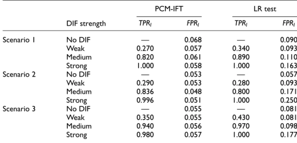
It can be seen from Table 2 that the proposed PCM-IFT approximately keeps the given significance level. In contrast, the LR test shows strongly inflated Type I error rates, in particular for strong DIF. In this simple case, the difference between PCM-IFT and LR test is the testing procedure. The LR test approach tests each item sepa-rately given all other items are free of DIF. The PCM-IFT pursues a sequential strat-egy that accounts for DIF found in previous steps. As was to be expected, TPRs on
Table 1. Number of Items (I), Number of Response Categories (k), and Number of DIF
Items (IDIF) for the Three Scenarios of Simulation I.
Simulation I I k IDIF
Scenario 1 8 3 1
Scenario 2 20 3 3
the item level increase with increasing strength of DIF for both methods. They are also slightly higher for the third scenario with five categories.
It should be noted that inflated type I error rates on the item level are also observed, when using the itemwise Wald test implemented in the function
Waldtest() of the R package eRm (Mair and Hatzinger, 2007). We prefer to report the results of the self-implemented LR-test, because the function Waldtest() uses separate tests for each threshold.
The FPRs on the variable level for PCM-IFT (Table 3) seem surprisingly high. However, bearing in mind that FPRs were controlled on the item and not on the vari-able level, the results make sense. If the probability of one item to be falsely classi-fied as DIF item is 0.05, then the probability that one or more out of 8 items are falsely classified as DIF item is: 1(0:958) = 10:663 = 0:337. For 20 items: 1(0:9520) = 10:358 = 0:642. Of course, this only holds for simulation I in which
there is only one covariate and each split is automatically made for this covariate. Consequently, FPRs on the variable level are much higher compared with the TREE-PCM procedure, in which they are controlled on the variable level, and therefore the significance level is mostly respected. It can further be seen, that also TPRs are much higher for PCM-IFT than for TREE-PCM. A TPR of 100 in Scenario 3 with weak DIF means that only in 10 % of the cases the present DIF is found. The reason might be that the ratio of DIF items to non-DIF items is very small in Scenarios 1 and 3. Therefore, for the detection of single items the power is much higher. Accordingly, in Scenario 2, where the ratio of DIF items to non-DIF items is higher) TREE-PCM performs better.
Table 2. Average True Positive and False Positive Rates for PCM-IFT and the LR Test Based
on 100 Replications (Simulation I).
DIF strength PCM-IFT LR test TPRI FPRI TPRI FPRI Scenario 1 No DIF — 0.068 — 0.090 Weak 0.270 0.057 0.340 0.093 Medium 0.820 0.061 0.890 0.110 Strong 1.000 0.058 1.000 0.163 Scenario 2 No DIF — 0.053 — 0.057 Weak 0.290 0.053 0.280 0.093 Medium 0.836 0.048 0.800 0.171 Strong 0.996 0.051 1.000 0.250 Scenario 3 No DIF — 0.055 — 0.081 Weak 0.350 0.055 0.430 0.081 Medium 0.940 0.056 0.970 0.098 Strong 0.980 0.057 1.000 0.177
Note. DIF = differential item functioning; TPR = true positive rate; FPR = false positive rate; PCM-IFT = item-focused trees based on the partial credit model; LR = likelihood ratio.
Simulation II: Three Different Covariates
In the second simulation study, we investigate how well the proposed method is able to detect the right DIF inducing covariate out of multiple present covariates. We con-sider scenarios withI= 8,k= 3 andIDIF= 1. Now, there are three different covariates
that possibly induce DIF—one binary variable x12 f0, 1g, one ordered factor
x2 2 f1, 2, 3, 4g, and one numeric covariatex32 f20,. . ., 50g. Variablex3could, for
example, represent the variable age. In each of the following scenarios, exactly one of these covariates induces DIF in one item. Again, all thresholds of one item are shifted in the same direction. There is one split-point cvj per item atcvj=xvmed. The
threshold parameters of the two subgroups are given by
gir(2)=gir(1)+lI(xpv.xvmed), r= 1, 2:
To obtain weak, medium, and strong DIF, parameterslare chosen in the same way as in the previous simulation.
Results. Figure 4 shows one estimated tree for Item 5 (the item with DIF), for the three different scenarios of Simulation II with strong DIF, respectively. In the chosen examples, the true underlying DIF structure was detected. In Scenario 1, DIF is induced byx1, in Scenario 2 byx2, and in Scenario 3 byx3. In these examples also, the true simulated split-points (2, 2 and 34), are correctly identified. In each scenario,
the true item parameters are g5(1)= (0:5, 0:5)T in the left node and
g5(2)= (0:5, 1:5)Tin the right node. It can be seen from the graphical representations
Table 3. Average TPRV andFPRV for TREE-PCM and PCM-IFT Based on 100 Replications
(Simulation I). DIF strength TREE-PCM PCM-IFT TPRV FPRV TPRV FPRV Scenario 1 No DIF — 0.080 — 0.410 Weak 0.100 — 0.490 — Medium 0.280 — 0.880 — Strong 0.930 — 1.000 — Scenario 2 No DIF — 0.050 — 0.680 Weak 0.140 — 0.850 — Medium 0.610 — 1.000 — Strong 1.000 — 1.000 — Scenario 3 No DIF — 0.040 — 0.390 Weak 0.100 — 0.590 — Medium 0.460 — 0.950 — Strong 1.000 — 0.980 —
Note. DIF = differential item functioning; TPR = true positive rate; FPR = false positive rate; PCM-IFT = item-focused trees based on the partial credit model; TREE-PCM = RaschTree partial credit model.
of the parameters in the leaves of the trees that the estimated parameters are quite close to the true ones.
To account for the multiple covariates in the model, the significance level at each node is divided by the number of covariates available at this node: a= 0:05=V. Tables 4 and Table 5 give an overview of the TPRs and FPRs based on 100 replica-tions for Simulation II.
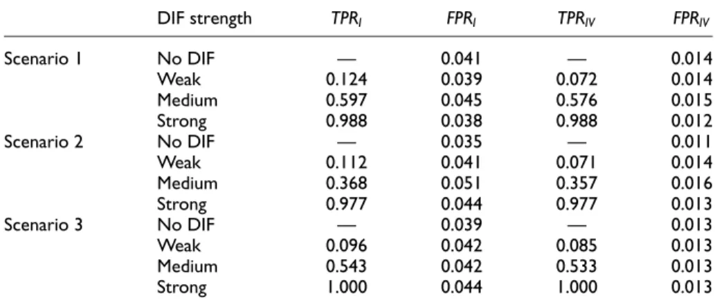
In Table 4, it can be seen that FPRs are always close to the given significance level demonstrating that the alpha level correction works quite well. For the combi-nation of items and variables they are necessarily smaller. From the first and the third columns in Table 4, one can conclude that almost in all cases where a split was per-formed, also the right variable was selected. On variable level (Table 5), FPRs again are higher than 0.05 but not as high as in simulation I. It is noteworthy that TREE-PCM is very conservative in this simulation which results in very small true and FPRs. Similar to simulation I, TPRs of PCM-IFT are much higher than those of TREE-PCM.
Simulation III: Nonhomogeneous DIF
In the third simulation, nonhomogeneous DIF is simulated in the settings withI= 8, k= 3, and IDIF= 1 with regard to one binary DIF-inducing covariate. Unlike in the
Figure 4. Estimation results for one example of the three scenarios of Simulation II with
three covariates and strong differential item functioning (DIF). The estimated item parametersg5r(1)andg5r(2)are visualized in each leaf of the trees.
previous simulations, threshold parameters now are not all shifted by an equal amount from the reference to the focal group, but half of the parameters is shifted to the left and the other half to the right. More precisely, since only the case of two threshold parameters per item was considered, the first threshold parameter is shifted to the left and the second to the right. As a result, the difference between threshold parameters,
Table 5. Average TPRV andFPRV for TREE-PCM and PCM-IFT Based on 100 Replications
(Simulation II). DIF strength TREE-PCM PCM-IFT TPRV FPRV TPRV FPRV Scenario 1 no DIF — 0.013 — 0.110 weak 0.030 0.025 0.154 0.113 medium 0.160 0.035 0.630 0.097 strong 0.870 0.025 0.988 0.075 Scenario 2 no DIF — 0.013 — 0.093 weak 0.060 0.015 0.153 0.122 medium 0.110 0.015 0.410 0.131 strong 0.700 0.025 0.977 0.102 Scenario 3 no DIF — 0.013 — 0.104 weak 0.040 0.015 0.202 0.090 medium 0.180 0.030 0.619 0.076 strong 0.970 0.025 1.000 0.096
Note. DIF = differential item functioning; TPR = true positive rate; FPR = false positive rate; PCM-IFT = item-focused trees based on the partial credit model; TREE-PCM = RaschTree partial credit model.
Table 4. Average True Positive and False Positive Rates for PCM-IFT Based on 100
Replications (Simulation II).
DIF strength TPRI FPRI TPRIV FPRIV Scenario 1 No DIF — 0.041 — 0.014 Weak 0.124 0.039 0.072 0.014 Medium 0.597 0.045 0.576 0.015 Strong 0.988 0.038 0.988 0.012 Scenario 2 No DIF — 0.035 — 0.011 Weak 0.112 0.041 0.071 0.014 Medium 0.368 0.051 0.357 0.016 Strong 0.977 0.044 0.977 0.013 Scenario 3 No DIF — 0.039 — 0.013 Weak 0.096 0.042 0.085 0.013 Medium 0.543 0.042 0.533 0.013 Strong 1.000 0.044 1.000 0.013
Note. DIF = differential item functioning; TPR = true positive rate; FPR = false positive rate; PCM-IFT = item-focused trees based on the partial credit model.
i.e. the category width changes from the reference to the focal group. The two thresh-old parameters are then given through:
gi1(2)=gi1(1)lI(xp= 1)
gi2(2)=gi2(1)+lI(xp= 1):
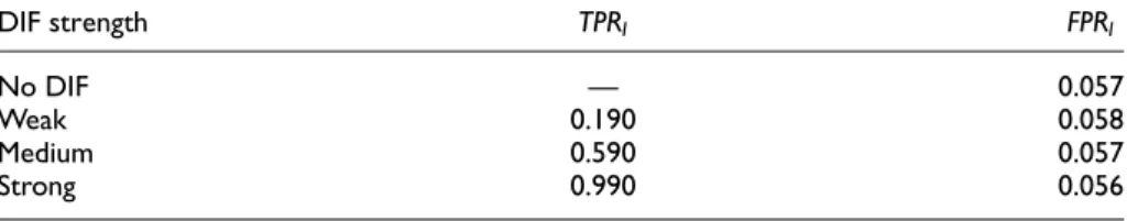
Results. Table 6 displays true and FPRs on the item level for PCM-IFT. Both, FPRs and TPRs are satisfactory and very similar to those in Simulation I, Scenario 1 where the same number of items and categories were used. Figure 5 shows one estimated tree for Item 5 (the item with DIF) for the setting with strong DIF of Simulation III, where the true underlying DIF structure was detected. In this scenario, with nonho-mogeneous DIF, the true item parameters are g5(1)= (0:5, 0:5)T in the left node andg5(2)= (1:5, 1:5)T in the right node. From the graphical representations of the
Figure 5. Estimation result for one example of Simulation III with one covariate and
nonhomogeneous differential item functioning (DIF) (strong setting). The estimated item parametersg5r(1)andg5r(2)are visualized in each leaf of the tree.
Table 6. Average True Positive and False Positive Rates for PCM-IFT Based on 100
Replications (Simulation III).
DIF strength TPRI FPRI
No DIF — 0.057
Weak 0.190 0.058
Medium 0.590 0.057
parameters in the leaves of the trees, it can be seen that the underlying nonhomoge-neous DIF structure is detected by the algorithm.
Concluding Remarks
We propose an approach to detect DIF in ordinal item response based on the PCM. By item-focused recursive partitioning, the proposed method allows for simultaneous detection of items and variables that are responsible for DIF. The results are small trees for each item that is not compatible with the PCM. Graphical representations of the threshold parameters in each terminal node enable an easy interpretation of the estimated effects and the differences between the detected groups. The simulations demonstrate that the proposed procedure works well, in particular, in settings where only few DIF items are present (which is usually the case in applications). The exist-ing TREE-PCM, however, is more suitable in cases where users assume most of the items to have DIF or simply want to test for DIF in the questionnaire without flagging the individual DIF items. Surprisingly, a comparison to the item wise LR-test reveals that this conventional method does not work well in the simple simulation scenario since it shows strongly inflated type I error rates. We can therefore conclude that the proposed PCM-IFT shows advantages over conventional methods (multiple covari-ates, no prespecification of subgroups) and has the additional benefit that it does not only tests for DIF but also automatically detects DIF items.
The proposed model explicitly tests DIF on theitem level. That means in each step the whole parameter vector H0:gi(1)gi(2)=0
is tested and if a split is performed, all the threshold parameters are estimated in both nodes without any restrictions. An alternative strategy would be to test for DIF in single thresholds. Then for fixed item and variable in each step one tests the hypothesesH0 :gir(1)gir(2)= 0, r= 1,. . .,k,
and selects the threshold that has the best fit. Accordingly, in each step only one threshold dir changes for one group. In future research, one might also consider a
homogeneous modeling approach, in which again all thresholds are shifted but now all in the same direction by an item-specific constantgi. Then, for example, after the
first split the item parameters in regionfxpv.cvgare defined bydi1+gi,. . .,dik+gi.
Both strategies are certainly worth investigating but the adoption of the existing proce-dure needs further research.
We restricted consideration to the widely used partial credit model. However, the basic concept can also be used to model DIF in alternative ordinal item response models, for example in the rating scale model (Andrich, 1978). In the rating scale model, the predictor has the formup(bi+tr), with item location parameterbiand
threshold parameter tr. With item-focused trees, the location parameter bi can be
replaced by gi(1)I(xpvcv) +gi(2)I(xpv.cv), the threshold parameter tr can be
replaced by ar(1)I(xpvcv) +ar(2)I(xpv.cv) or both parameters can be modified
simultaneously. Fitting of corresponding models requires the development of tailored testing strategies and appropriate estimation tools, which is beyond the scope of this article.
All the results presented in this article were obtained by means of an R program (as described in the Computation of Estimates section), which is available from the authors and will soon be available in an extended version of the R add-on package DIFtree (Berger, 2016) on CRAN.
Declaration of Conflicting Interests
The author(s) declared no potential conflicts of interest with respect to the research, authorship, and/or publication of this article.
Funding
The author(s) received no financial support for the research, authorship, and/or publication of this article.
References
Andersen, E. B. (1973). Conditional inference and models for measuring. Copenhagen, Denmark: Metalhygiejnish Forlag.
Andrich, D. (1978). A rating formulation for ordered response categories.Psychometrika,43, 561-573.
Andrich, D. (2013). An expanded derivation of the threshold structure of the polytomous Rasch model that dispels any threshold disorder controversy. Educational and Psychological Measurement,73, 78-124.
Andrich, D. (2015). The problem with the step metaphor for polytomous models for ordinal assessments.Educational Measurement: Issues and Practice,34(2), 8-14.
Berger, M. (2016). DIFtree: Item focused trees for the identification of items in differential item functioning. R package version 2.1.4.
Holland, P. W., & Thayer, D. T. (1988). Differential item performance and the Mantel-Haenszel procedure. In H. Wainer & H. I. Brown (Eds.), Test validity (pp. 129-145). Hillsdale, NJ: Lawrence Erlbaum.
Holland, P. W., & Wainer, H. (1993).Differential item functioning. Hillsdale, NJ: Lawrence Erlbaum.
Hothorn, T., & Lausen, B. (2003). On the exact distribution of maximally selected rank statistics.Computational Statistics and Data Analysis,43, 121-137.
Kim, S.-H., Cohen, A. S., & Park, T.-H. (1995). Detection of differential item functioning in multiple groups.Journal of Educational Measurement,32, 261-276.
Komboz, B., Strobl, C., & Zeileis, A. (2018). Tree-based global model tests for polytomous Rasch models. Educational and Psychological Measurement, 78, 128-166. doi:10.1177/ 0013164416664394
Lord, F. M. (1980).Applications of item response theory to practical testing problems. New York, NY: Routledge.
Magis, D., Be`land, S., Tuerlinckx, F., & De Boeck, P. (2010). A general framework and an R package for the detection of dichotomous differential item functioning.Behavior Research Methods,42, 847-862.
Magis, D., Tuerlinckx, F., & De Boeck, P. (2015). Detection of differential item functioning using the lasso approach.Journal of Educational and Behavioral Statistics,40, 111-135.
Mair, P., & Hatzinger, R. (2007). Extended Rasch modeling: The eRm package for the application of IRT models in R.Journal of Statistical Software,20(9), 1-20.
Masters, G. N. (1982). A Rasch model for partial credit scoring.Psychometrika,47, 149-174. Masters, G. N., & Wright, B. (1984). The essential process in a family of measurement models.
Psychometrika,49, 529-544.
Millsap, R. E. (2012).Statistical approaches to measurement invariance. New York, NY: Routledge.
Ostendorf, F., & Angleitner, A. (2004).NEO-Perso¨nlichkeitsinventar nach Costa und McCrae, Revidierte Fassung. [NEO Personality Inventory based on Costa and McCrae, revised version (NEO-PI-R)] Go¨ttingen, Germany: Hogrefe.
Penfield, R. D. (2007). Assessing differential step functioning in polytomous items using a common odds ratio estimator.Journal of Educational Measurement,44, 187-210.
Penfield, R. D. (2008). An odds ratio approach for assessing differential distractor functioning effects under the nominal response model. Journal of Educational Measurement, 45, 247-269.
Penfield, R. D., & Algina, J. (2003). Applying the Liu-Agresti estimator of the cumulative common odds ratio to DIF detection in polytomous items. Journal of Educational Measurement,40, 353-370.
Penfield, R. D., & Camilli, G. (2006). Differential item functioning and item bias. In C. Rao & S. Sinharay (Eds.), Handbook of statistics: Vol. 26. Psychometrics (pp. 125-167). Amsterdam, Netherlands: Elsevier.
Raju, N. S. (1988). The area between two item characteristic curves. Psychometrika, 53, 495-502.
Schauberger, G., & Tutz, G. (2016). Detection of differential item functioning in Rasch models by boosting techniques.British Journal of Mathematical and Statistical Psychology, 69, 80-103.
Shih, Y.-S. (2004). A note on split selection bias in classification trees. Computational Statistics and Data Analysis,45, 457-466.
Shih, Y.-S., & Tsai, H. (2004). Variable selection bias in regression trees with constant fits.
Computational Statistics and Data Analysis,45, 595-607.
Strobl, C., Boulesteix, A.-L., & Augustin, T. (2007). Unbiased split selection for classification trees based on the Gini index.Computational Statistics and Data Analysis,52, 483-501. Strobl, C., Kopf, J., & Zeileis, A. (2015). Rasch trees: A new method for detecting differential
item functioning in the Rasch model.Psychometrika,80, 289-316.
Thissen, D., Steinberg, L., & Wainer, H. (1993). Detection of differential item functioning using the parameters of item response models. In P. W. Holland & H. Wainer (Eds.),
Differential item functioning(pp. 67-113). Hillsdale, NJ: Lawrence Erlbaum.
Tutz, G., & Berger, M. (2016). Item-focussed trees for the identification of items in differential item functioning.Psychometrika,81, 727-750.
Tutz, G., & Schauberger, G. (2015). A penalty approach to differential item functioning in Rasch models.Psychometrika,80, 21-43.
Yee, T. W. (2010). The VGAM package for categorical data analysis.Journal of Statistical Software,32(10), 1-34.
Yee, T. W. (2014). VGAM:Vector generalized linear and additive models. R package version 0.9-4.
Yee, T. W., & Wild, C. J. (1996). Vector generalized additive models.Journal of the Royal Statistical Society B,58, 481-493.